mbsolve: An open-source solver tool for the Maxwell-Bloch equations

Abstract

The Maxwell-Bloch equations are a valuable tool to model light-matter interaction, where the application examples range from the description of pulse propagation in two-level media to the elaborate simulation of optoelectronic devices, such as the quantum cascade laser (QCL). In this work, we present mbsolve, an open-source solver tool for the Maxwell-Bloch equations. Here, we consider the one-dimensional Maxwell’s equations, which are coupled to the Lindblad equation. The resulting generalized Maxwell-Bloch equations are treated without invoking the rotating wave approximation (RWA). Since this full-wave treatment is computationally intensive, we provide a flexible framework to implement different numerical methods and/or parallelization techniques. On this basis, we offer two solver implementations that use OpenMP for parallelization.

1 Introduction

In the field of nonlinear optics, the Maxwell-Bloch equations are a valuable tool to model light-matter interaction [1]. Originally devised to describe the behavior of magnetic moments of nuclei in a magnetic field [2], the Bloch equations soon found further application in which the dynamics of a two-level quantum mechanical system in resonance with an optical field are described [3, 4, 5]. This version is often referred to as optical Bloch equations and, coupled with Maxwell’s equations for the optical field, was successfully applied to model nonlinear phenomena such as self-induced transparency [6, 7]. Later, a generalized form of the optical Bloch equations that considers an arbitrary number of energy levels was derived [8]. Instances of this form for three energy levels have been used e.g., to describe electromagnetically induced transparency and the related slow light propagation [9, 10]. Similarly, further application examples of this generalized form can be related to the propagation of light in different media, and considering quantum mechanical systems with two [11, 12, 13], three [14, 15] or six [16] energy levels, respectively.

While in earlier studies the media considered were mostly of gaseous form, advances in nanotechnology paved the way for solid state optoelectronic devices that exhibit (at least partially) coherent light-matter interaction, as is adequately described by the Maxwell-Bloch equations [17]. Here, the quantum cascade laser (QCL) [18, 19] is a notable example. In many studies (e.g., [20, 21, 22, 23, 24, 25, 26, 27, 28, 29, 30, 31]), its dynamical behavior was simulated in this framework. Also quantum dot devices have been extensively modeled based on Maxwell-Bloch equations [32, 33, 12, 34]. For a detailed overview of the applications, the reader is referred to our recent review paper [17].

In the majority of related studies, the rotating wave approximation (RWA) in combination with the slowly varying envelope approximation (SVEA) is invoked. Naturally, these approximations may omit certain features of the solution [11]. We assume that those features are crucial in the scope of simulations of quantum cascade laser frequency combs [35, 36], which is the main application of the Maxwell-Bloch equations in our research. Hence, we aim to avoid the RWA and SVEA.

It should be noted that even when those approximations are used, analytical solutions are not generally available. As a consequence, we need to resort to numerical methods and solver tools that implement them. Although several numerical approaches for the Maxwell-Bloch equations have been discussed and compared in related literature [11, 37, 38, 15, 17, 16, 39, 40, 41, 42, 43], there is no definitive statement on what the best approach is. Also, just as with many problems in science and engineering, it is improbable that a single numerical method can cover all use cases. For example, while invoking the RWA/SVEA may not be suitable for quantum cascade laser frequency combs, it is perfectly reasonable for a multitude of problems. Therefore, the solver tool should provide support for multiple numerical methods in order to evaluate and compare different approaches. Here, a small and flexible code base is beneficial for rapid prototyping.

At the same time, the tool should permit productive usage with established numerical methods in the scope of our research, which leads to the following requirements. As already stated, a full-wave treatment of the optical field is desired (i.e., the rotating wave approximation should not be invoked). Secondly, as the full-wave treatment is computationally more intensive, the resulting numerical operations should be efficiently executed in parallel. Then, the solver should be able to deal with multiple sections of different materials, flexible initial and boundary conditions, source terms, and an arbitrary number of energy levels. Finally, the source code of the solver should be publicly available in order to allow extensions of the software and to improve the reproducibility of simulation results.

Unfortunately, the majority of the solver tools used in related work are not publicly available (e.g., in [11, 37, 38, 15, 16, 39]). In the following we discuss the few exceptions to that rule. For example, the Electromagnetic Template Library (EMTL) [44] is a free C++ library with Message Passing Interface (MPI) support and has been used e.g., to model single quantum emitters [40]. However, it is only available in binary form which makes it impossible to extend the library and port it to new computing architectures. The Freetwm [45] project is an open-source MATLAB code that solves the 1D Maxwell-Bloch equations. But to the best of our knowledge, it uses the rotating wave approximation and does not support alternative numerical methods. Also, solvers written and executed in MATLAB typically feature inferior performance than implementations in compiled languages such as C++. Finally, the open-source project MEEP [46] is a fully versed finite-difference time-domain (FDTD) solver for Maxwell’s equations with parallelization support (using MPI) and a flexible user interface. Also, it features support for multi-level quantum mechanical systems. It is widely accepted in the simulation community and, therefore, it is a promising project to base our future simulations onto. But one has to acknowledge that the evaluation and comparison of different numerical methods for the Maxwell-Bloch equations is hardly possible with such a large code base.

With this overview of existing approaches in mind, we decided to start developing our own project named mbsolve. The minimal and flexible code base already allowed comparisons of different numerical methods [41, 42, 43], as well as a discussion of their efficiency on parallel architectures [47]. Subsequently, the mbsolve project has been used productively in an investigation of harmonic mode locking in terahertz quantum cascade lasers [48] and the modeling of terahertz frequency combs interacting with a graphene-coated reflector [49]. However, it has not yet been introduced to potential users who wish to use this simulation software for their applications. In the work at hand, we would like to make up for this and present the mbsolve project.

In the following section, we introduce the Maxwell-Bloch equations as they are used in the scope of the mbsolve software, and discuss the different numerical methods that are employed to solve them. In Section 3, we present the implementation of mbsolve and discuss in detail the fundamental components. Namely, those are the basic library that provides the description of a simulation setup, an implementation of a solver using the OpenMP standard for parallelization, and a library that exports simulation results into the HDF5 format. In Section 4, we verify the correct operation of our implementation and discuss the features of the mbsolve software with the help of four application examples from related literature. Finally, after a short summary we conclude in Section 5 with an outlook on possible extensions of the software.

2 The Maxwell-Bloch equations

As already outlined, the Maxwell-Bloch equations describe the interaction of an electromagnetic field with quantum mechanical systems. In the most general picture, the electric field $\boldsymbol{E}(\boldsymbol{r},t)$ and the magnetic field $\boldsymbol{H}(\boldsymbol{r},t)$ depend on the three-dimensional space coordinate $\boldsymbol{r}$ and time $t$. The quantum mechanical systems are assumed to be uniformly distributed over space and are generally represented by the density matrix $\hat{\rho}(\boldsymbol{r},t)$. While the electromagnetic field is treated classically using Maxwell’s equations (in 3D), the density matrix is a concept from quantum mechanics. Its time evolution is governed by a master equation of the form

$$\partial_{t}\hat{\rho}=-\mathrm{i}\hbar^{-1}\left[\hat{H},\hat{\rho}\right]+\mathcal{D}(\hat{\rho}),$$ (1)

where $\hbar$ is the reduced Planck constant and $[\cdot,\cdot]$ denotes the commutator. The Hamiltonian $\hat{H}=\hat{H}_{0}-\hat{\boldsymbol{\mu}}\boldsymbol{E}$ consists of the static Hamiltonian $\hat{H}_{0}$ and the interaction term $\hat{\boldsymbol{\mu}}\boldsymbol{E}$, where $\hat{\boldsymbol{\mu}}$ is the dipole moment operator. The superoperator $\mathcal{D}(\hat{\rho})$ accounts for the non-unitary contribution to the time evolution of the density matrix. Its form also specifies the type of master equation. For example, if the superoperator is given in Lindblad form, Eq. (1) is referred to as Lindblad equation. At this point, the quantum mechanical systems are controlled by the electromagnetic field. The interaction cycle is completed by the introduction of a polarization term

$$\partial_{t}\boldsymbol{P}=n_{\mathrm{3D}}\operatorname{Tr}\{\hat{\boldsymbol{\mu}}\partial_{t}\hat{\rho}\}$$ (2)

that enters Ampere’s law in Maxwell’s equations. Here, $n_{\mathrm{3D}}$ is the density of quantum mechanical systems, and $\operatorname{Tr}\{\}$ is the trace operation [17].

2.1 Generalized Maxwell-Bloch equations in 1D

The resulting three-dimensional form of the Maxwell-Bloch equations is quite complex. In the scope of this work we address a simplified version that is relevant for two classes of applications. The first class consists of simulation models in which the plane wave approximation [50] is a reasonable assumption. Those models can be found frequently in related literature (e.g., [11, 16, 51]). The second class of applications contains the simulation of optoelectronic devices with a waveguide geometry that permits the separation of transversal and longitudinal modes. As a consequence, only the propagation direction has to be considered in the Maxwell-Bloch equations, whereas the change in transversal directions is accounted for using an effective refractive index. A detailed description of this procedure is given in [17].

The simplified version of Maxwell-Bloch equations can be written in terms of the field components $E_{z}(x,t)$ and $H_{y}(x,t)$, where $x$ is the propagation direction, and $y$, $z$ are the transversal coordinates. Then, Maxwell’s equations can be reduced to equations for the time evolution of the electric field

$$\partial_{t}E_{z}=\epsilon^{-1}\left(-\sigma E_{z}-\Gamma\partial_{t}P_{z}+\partial_{x}H_{y}\right)$$ (3)

and the magnetic field

$$\partial_{t}H_{y}=\mu^{-1}\partial_{x}E_{z},$$ (4)

where the conductivity $\sigma$, the permittivity $\epsilon=\epsilon_{0}\epsilon_{\mathrm{r}}$, and the permeability $\mu=\mu_{0}\mu_{\mathrm{r}}$ can be related to a (generally complex) effective refractive index. Additionally, the overlap factor $\Gamma$ is introduced, which accounts for a partial overlap of the transversal mode with the quantum mechanical systems and can be set to unity in cases where it is not required. The effective refractive index and the overlap factor are commonly used in optoelectronic device simulations and take into account the properties of the bulk material(s) in the setup as well as the waveguide geometry (if any). Generally, they depend on the position $x$ and the frequency, which applies here for the material parameters $\epsilon$, $\sigma$, $\mu$ and $\Gamma$. We note that the frequency dependence reflects the chromatic dispersion of the background medium, which combines waveguide and bulk dispersion. In the work at hand, we ignore this frequency dependence but note that the inclusion of the background dispersion should be in the focus of future work. The dispersion that stems from the quantum mechanical systems, on the other hand, is included in the polarization $\boldsymbol{P}$ and will be considered.

The variation of the material parameters in propagation direction is usually piecewise constant, in which case different regions of materials can be used to address this dependence. For each region, Eqs. (3) and (4) describe the electromagnetic field, where the material parameters are then constants. Within this model, the quantum mechanical systems are distributed only in the propagation direction and can be represented by the density matrix $\hat{\rho}(x,t)$. Furthermore, the dipole moment operator is now assumed to have only one non-zero component $\hat{\mu}_{z}$ [17]. Therefore, the polarization contribution that stems from the quantum mechanical systems can be written as

$$\partial_{t}P_{z}=n_{\mathrm{3D}}\operatorname{Tr}\{\hat{\mu}_{z}\partial_{t}\hat{\rho}\},$$ (5)

and the time evolution of the density matrix is described by the master equation

$$\partial_{t}\hat{\rho}=-\mathrm{i}\hbar^{-1}\left[\hat{H}_{0}-\hat{\mu}_{z}E_{z},\hat{\rho}\right]+\mathcal{D}(\hat{\rho}).$$ (6)

Now, as the system of partial differential equations is introduced, it is necessary to specify the initial and boundary conditions. The electric and magnetic fields require initial values $E(x,t=0)$ and $H(x,t=0)$, respectively. While many setups simply assume both to be zero, the fields may be initialized with random values to model spontaneous emission. The latter is typically applied during the simulation of lasers. As to boundary conditions, it is generally assumed that the electromagnetic wave is reflected with a certain reflectivity $R$ at the simulation domain boundary. This assumption covers the case of perfect ($R=1$) and semi-transparent ($0<R<1$) mirrors, which are often considered in optoelectronic devices, as well as perfectly matched layer (PML) boundary conditions ($R=0$). It should be noted that the reflectivity values of the two boundaries $R_{1}\neq R_{2}$ may be different. Since the master equation (6) does not include a spatial derivative, only the initial value of the density matrix at each point is required, such as thermal equilibrium (lowest energy level has the largest population) or inversion (some higher energy level, the so-called upper laser level, has the largest population). Finally, we note that source terms are often included in related literature. For example, an incoming electromagnetic pulse of Gaussian or sech shape is modeled by a source term in the electric field.

Together with those initial and boundary conditions, the differential equations (3)-(6) form the generalized Maxwell-Bloch equations in 1D. If we reduce the model further by ignoring the propagation effects altogether, the equation system is nothing more than the master equation (6) that describes the time evolution for a single quantum mechanical system. As a consequence, the software project presented in the work at hand may also serve as solver for e.g., the Lindblad equation. Starting again from the one-dimensional version, we note that the generalized Maxwell-Bloch equations are able to treat an arbitrary number of energy levels $N$. The original Maxwell-Bloch equations can be derived by setting $N=2$. At this point, the rotating wave approximation (RWA) is usually applied in order to reduce further the complexity of the equation system. However, we shall not go along this way, but discuss numerical methods that are able to solve the one-dimensional generalized Maxwell-Bloch equations.

2.2 Numerical treatment

Here, we can divide the discussion in three parts. The first part is dedicated to numerical methods that solve Maxwell’s equations. As already stated above, we focus on methods that solve the full wave equations, i.e., that do not invoke the rotating wave or slowly varying envelope approximation. Another part deals with the numerical treatment of the master equation (6). In between, the coupling of both parts is discussed. Throughout this subsection, we base on our recent review paper, in which the state of the art in numerical methods for the Maxwell-Bloch equations is reviewed in more detail [17].

The majority of related work uses on the finite-difference time-domain (FDTD) method to solve Maxwell’s equations. Clearly, it is one of the standard approaches in computational electromagnetics, and its simplicity allows straightforward implementation of source terms and sharp material boundaries. As disadvantages, its numerical dispersion and the need for a constant spatial discretization must be mentioned. The usual remedy for the numerical dispersion is to decrease the spatial and temporal grid spacing, which in turn increases the computational workload. As an alternative, the pseudo-spectral time-domain (PSTD) method has been used in related work [39, 16]. The PSTD method calculates the spatial derivatives accurately in a pseudo-spectral domain, in which they are reduced to mere multiplication operations. Thereby, the spatial contribution of the numerical dispersion is eliminated and the temporal contribution is significantly reduced. However, this comes at the cost of potentially expensive calls to the fast Fourier transform (FFT), and complex implementations of boundary conditions and source terms. The need of the FDTD method for a constant spatial discretization can lead to inefficient discretization patterns in setups with different media. The grid spacing must be chosen to suit the medium with the largest effective refractive index and will be unnecessarily small for media with smaller refractive indices. Numerical methods that adapt the spatial discretization variably to the problem are used to solve Maxwell’s equations, but to the best of our knowledge they have not been applied in the scope of the Maxwell-Bloch equations. In this work, we follow the majority of related literature and focus on the FDTD method. Nevertheless, the resulting software should be designed that it can serve as basis for implementations of alternative numerical methods, such as the PSTD method or methods that use adaptive spatial grids.

Figure 1 shows the standard Yee grid of the FDTD method, i.e., the discretization of the electric field $E_{z}$ and magnetic field $H_{y}$ as function of the spatial index $m$ and the temporal index $n$. The main feature of the Yee grid is that the electric and magnetic field are staggered in time and space. This clever choice leads to the central difference equations [52]

$$\frac{E_{z}^{m,n+1}-E_{z}^{m,n}}{\Delta t}= -\epsilon^{-1}\sigma\frac{E_{z}^{m,n+1}+E_{z}^{m,n}}{2}-\epsilon^{-1}\Gamma\left(\partial_{t}P_{z}\right)^{m,n+1/2}$$ (7)

$$+\epsilon^{-1}\frac{H_{y}^{m+1/2,n+1/2}-H_{y}^{m-1/2,n+1/2}}{\Delta x}$$

and

$$\frac{H_{y}^{m+1/2,n+1/2}-H_{y}^{m+1/2,n-1/2}}{\Delta t}=\mu^{-1}\frac{E_{z}^{m+1,n}-E_{z}^{m,n}}{\Delta x}$$ (8)

for Eqs. (3) and (4), respectively. Here, $\Delta x$ is the spatial grid point size, and $\Delta t$ is the temporal discretization size. As to the discretization of the density matrix, there are two choices, which are referred to as weak and strong coupling, respectively [38]. The difference between those choices is the temporal discretization, where strong coupling uses the same discretization points for both the electric field and the density matrix. Weak coupling, as depicted in Fig. 1, uses different discretization points, which are staggered in time.

myline=[line cap=round,line join=round, ultra thick]; cs=[myline, black, -¿, ¿=stealth]; [cs] (0, 0) – (1, 0) node[above] $x$; [cs] (0, 0) – (0, -1) node[left] $t$; ıin 0, …, 7 ȷin 0, …, 3 (hıȷ) at (0.5 + 1.0*ı, -0.5 - 1.0*ȷ) ; [myline, sipblue] (hıȷ) circle[radius=3pt]; ıin 0, …, 6 ȷin 0, …, 3 (eıȷ) at (1.0 + 1.0*ı, -1.0 - 1.0*ȷ) ; [myline, siporange] (eıȷ) ++ (-3pt, 0) – ++(6pt, 0); [myline, siporange] (eıȷ) ++ (0, -3pt) – ++(0, 6pt); ıin 0, …, 6 ȷin 0, …, 3 (dıȷ) at (1.0 + 1.0*ı, -0.5 - 1.0*ȷ) ; [myline, sipgreen] (dıȷ) ++(-3pt, -3pt) rectangle ++(6pt, 6pt); [cs] ($(h30)+(0,-5pt)$) – ($(h31)+(0,5pt)$); [cs] ($(e20)+(3pt,-3pt)$) – ($(h31)+(0,5pt)$); [cs] ($(e30)+(-3pt,-3pt)$) – ($(h31)+(0,5pt)$); [cs] ($(e51)+(0,-5pt)$) – ($(e52)+(0,5pt)$); [cs] ($(h52)+(3pt,-3pt)$) – ($(e52)+(0,5pt)$); [cs] ($(h62)+(-3pt,-3pt)$) – ($(e52)+(0,5pt)$); [cs, out=-30, in=60] ($(d52)+(5pt,0)$) to ($(e52)+(5pt,0)$); [cs] ($(d12)+(0,-5pt)$) – ($(d13)+(0,5pt)$); [cs, out=-30, in=60] ($(e12)+(5pt,0)$) to ($(d13)+(5pt,0)$);

Figure 1: The standard Yee grid of the FDTD method combined with the discretization of the density matrix with respect to time and space. Electric and magnetic field are denoted with orange crosses and blue circles, respectively. The density matrix discretization is marked using green squares. The arrows indicate the data dependencies during the update of three quantities. Reprinted from Riesch M., et al. [47] (CC BY 4.0).

Regardless of the coupling, the remaining task is the update step of the density matrix from one time value to the next one. This operation can be formally written as

$$\hat{\rho}_{n+1/2}=\exp(\mathcal{L}\Delta t)\hat{\rho}_{n-1/2}\approx\mathcal{U}_{n}(\hat{\rho}_{n-1/2}),$$ (9)

where the Liouvillian superoperator $\mathcal{L}$ represents the right-hand side of Eq. (6). The solution of Eq. (6) for a certain time step $\Delta t$ can be specified with the help of the exponential superoperator. In practice, however, this formal expression can only be approximated using a certain update operation $\mathcal{U}_{n}$, which serves as placeholder for different numerical methods. Indeed, several candidates with different accuracies and complexities have been suggested in related literature, which can be roughly divided into three groups [17, 53]. Several studies use the Crank-Nicolson method to solve the master equation, where the implicit nature of this method is usually resolved using a predictor-corrector approach [11, 14]. However, it has been pointed out that neither the Crank-Nicolson method nor the predictor-corrector approach guarantees the preservation of the positivity of the density matrix [37, 53]. Alternatively, higher-order Runge-Kutta methods have been employed (e.g., in [15, 12]). Although they typically feature higher accuracy than the first group of methods, there is still no guarantee that the positivity of the density matrix is preserved. The third group of approaches revolves around solving the master equation exactly for one time step, which is related to calculating matrix exponentials. Since this operation is very costly, operator splitting techniques are often applied [37, 38, 16]. This group of methods is the one with the highest computational complexity but guarantees the preservation of the density matrix properties. For a thorough review of numerical methods for the master equation the reader is referred to our recent reviews [17, 53]. We would like to point out, however, that there is still no definite answer on what the best numerical method is. This question has been in the focus of recent work [41, 42, 43] and will be discussed elsewhere in more detail.

In mbsolve, the established operator splitting method presented in [37] is implemented for productive usage and as reference for promising new methods. This method guarantees to preserve the properties of the density matrix and is therefore well-suited for long-term simulations, which are often required in the scope of the simulation of optoelectronic devices. Additionally, there is an adapted form of the operator splitting method [54] that is currently evaluated. As we have already pointed out, one of the primary design goals of mbsolve is the support of different numerical methods, which naturally includes different approaches to solve the master equation. Thereby, mbsolve will aid the comparison between various promising candidates.

3 Implementation of mbsolve

In this section, we present the architecture and the implementation details of the mbsolve software. The modular architecture was designed with the requirements from Section 1 in mind, which we revisit briefly in the following. As we already stated, it is crucial that mbsolve supports different numerical methods for the Maxwell-Bloch equations. We note that a flexible way to combine methods for Maxwell’s equations and methods for the master equation would be beneficial. Then, for example, it would not be required to implement the FDTD method multiple times when evaluating different algorithms to solve the master equation. Similarly, there are different parallelization techniques (OpenMP for shared memory systems, MPI for distributed memory systems, CUDA for NVIDIA graphics processing units (GPU), etc.), and mbsolve should be able to handle different techniques. Thereby, available simulation hardware can be targeted and exploited. A preliminary study found that the Maxwell-Bloch equations can be efficiently solved on GPUs [55], but the software should also work on a regular desktop PC without a high-end graphics card. As already mentioned, we found that a small, yet flexible and extensible, code base is beneficial in order to achieve this. Finally, we envisage to share the resulting software project with the scientific community. Here, several measures must be taken to guarantee that other researchers can acquire, install and use the software [56]. While we discuss those measures in more detail below, the fundamental decision is the choice of programming language. We decided to use the C++ programming language for performance reasons, and offer bindings for Python in order to provide an easy-to-use interface for the researchers. Both programming languages are established in the scientific community and should constitute a reasonable choice [56].

During the implementation of the mbsolve software, the required flexibility was guaranteed by modularization and clearly defined interfaces. Those design criteria lead to the architecture depicted in Fig. 2. The mbsolve-lib base library constitutes the fundamental part of the software, as it provides an object oriented framework to define a simulation setup as well as the infrastructure to add solver and writer components. As the name suggests, the solver components implement numerical methods that solve the specified simulation setup using different parallelization techniques. After the solver has completed its work, the writer component is responsible for writing the simulation results into a file. In principle, writers for any file format can be implemented. However, we found that the Hierarchical Data Format (HDF) fulfills all of our needs.

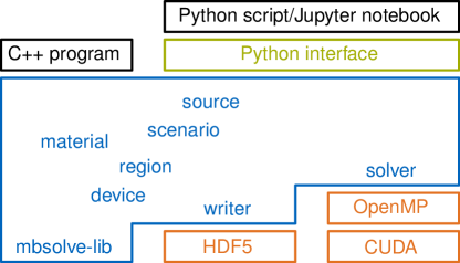
Figure 2: Overview of the mbsolve project. Reprinted from M. Riesch, The QCL Stock Image Project [57] (CC BY 4.0).

In the following, we present in more detail the mbsolve-lib base library, two exemplary solvers based on the OpenMP standard and the numerical methods described in [37, 54], respectively, and the writer for the HDF5 file format. Subsequently, we discuss the measures taken to create a sustainable open-source software project out of mbsolve.

3.1 The mbsolve-lib base library

The object oriented framework that describes a simulation setup can be divided into two parts. The device part contains all properties of a setup that are static. These properties include, for example, the composition of the device under simulation in terms of regions and materials. The dynamic properties, on the other hand, are grouped into a scenario. For instance, simulation properties, such as the number of grid points used, or source terms are defined in the scenario. Thereby, it is possible to simulate the same device under different conditions, which was used, e.g., during the investigation of seeding effects in a quantum cascade laser [24]. After device and scenario are defined, the user can pass them to a solver, which calculates the simulation results, and optionally to a writer, which exports the results to a file.

3.1.1 Device setup and boundary conditions

The device is represented by a class of the same name. It contains a collection of region objects, which models a section of the device in which the material parameters are constant. A region is defined by the $x_{\mathrm{start}}$ and $x_{\mathrm{end}}$ coordinates as well as a pointer to a certain material. The envisaged materials have to be present in a static collection when the region is created. Thereby, material parameters are not directly stored in the regions. This enables the efficient treatment of periodic structures, where only few materials are repeatedly used in many different regions.

Each material is an instance of the eponymous class, which contains the electromagnetic properties as well as the description of the quantum mechanical systems. The former consist of the permittivity $\epsilon$, the permeability $\mu$, the overlap factor $\Gamma$, and the linear loss term

$$\alpha_{0}=\frac{\sigma}{2\epsilon c}=\sqrt{\frac{\mu}{\epsilon}}\frac{\sigma}{2},$$ (10)

which is related to the conductivity $\sigma$ [50]. Here, $c=(\mu\epsilon)^{-1/2}$ is the speed of light in the material. The latter is incorporated as pointer to the class qm_description, which represents a quantum mechanical system. Here, the usage of a pointer allows polymorphism, i.e., the quantum mechanical description can assume different forms.

In the general form, this description requires the density of quantum mechanical systems $n_{\mathrm{3D}}$, the Hamiltonian $\hat{H}_{0}$ and the dipole moment operator $\hat{\mu}_{z}$, as well as the superoperator $\mathcal{D}$. For $\hat{H}_{0}$ and $\hat{\mu}_{z}$ the class qm_operator can be used. Since quantum mechanical operators can be expressed as Hermitian matrices, it is sufficient to store the real entries of the main diagonal as well as the complex entries of the upper triangle of the matrix. For example, a diagonal Hamiltonian

$$\hat{H}_{0}=\begin{bmatrix}\omega_{1}&0&0\\ 0&\omega_{2}&0\\ 0&0&\omega_{3}\end{bmatrix}$$ (11)

can be created from a real vector $[\omega_{1},\omega_{2},\omega_{3}]$. In this case it is not necessary to provide a complex vector for the off-diagonal elements since they are set to zero by default. On the other hand, for a dipole moment operator

$$\hat{\mu}_{z}=\begin{bmatrix}0&\mu_{12}&\mu_{13}\\ \mu_{21}&0&\mu_{23}\\ \mu_{31}&\mu_{32}&0\end{bmatrix}$$ (12)

the main diagonal elements are defined by the real vector $[0,0,0]$ and the off-diagonal elements are represented by the complex vector $[\mu_{12},\mu_{13},\mu_{23}]$.

The treatment of superoperators is more complex, since the action of the superoperator on a quantum mechanical operator must be determined. Also, different choices of the superoperator are reasonable. Therefore, we implemented the class qm_superoperator and derived a sub-class qm_lindblad_relaxation that represents the resulting Lindblad superoperator. This approach allows future extensions, yet covers all current application examples, since the Lindblad form of the master equation is the most general Markovian description [58]. The Lindblad superoperator [59, 60] can be written as

$$\mathcal{D}(\hat{\rho})=\sum_{i,j=1}^{N^{2}-1}c_{ij}\left[\hat{F}_{i}\hat{\rho}\hat{F}_{j}^{\dagger}-\frac{1}{2}\left(\hat{F}_{j}^{\dagger}\hat{F}_{i}\hat{\rho}+\hat{\rho}\hat{F}_{j}^{\dagger}\hat{F}_{i}\right)\right],$$ (13)

where $N$ is the dimension of the underlying Hilbert space $\mathcal{H}$, i.e., the number of energy levels under consideration. Furthermore, the coefficients $c_{ij}$ form a positive semi-definite matrix $C$ and the traceless operators $\hat{F}_{i}$ constitute an orthonormal basis of the space $B(\mathcal{H})$ of all bounded operators on the Hilbert space $\mathcal{H}$ with the restriction that $\hat{F}_{N^{2}}$ is proportional to the identity operator. It should be noted that the choice of the operators $\hat{F}_{i}$ is not unique, as the resulting dynamical behavior is invariant under certain transforms, e.g., any unitary transform [58]. Preferably, we choose a set of operators that allows a straightforward physical interpretation of the dissipation superoperator. Such a suitable choice is presented in [61] and consists of $N(N-1)$ operators of the form $\hat{F}_{k}=\ket{i}\bra{j}$, where the indices $i,j\in[1;N],i\neq j$ are mapped to the index $k\in[N;N^{2}-1]$, and $N-1$ diagonal operators of the form

$$\hat{F}_{k}=\frac{1}{\sqrt{k(k+1)}}\left(\sum_{s=1}^{k}\ket{s}\bra{s}-k\ket{k+1}\bra{k+1}\right),$$ (14)

where $k\in[1;N-1]$. The latter group of operators can be related to the Pauli matrices and Gell-Mann matrices (for $N=2$ and $N=3$, respectively). By plugging the operator expressions into Eq. (13), it becomes apparent that the time evolution of the populations is determined by the operators $\hat{L}_{k},k\in[N;N^{2}-1]$ alone, which are in the following referred to as relaxation operators. As the name suggests, each operator represents a relaxation or scattering process from an energy level $\ket{i}$ to another level $\ket{j}$ with the scattering rate $\gamma_{ji,i\neq j}$, where the mapping between the indices $i,j$ and $k$ mentioned before has been reverted. Assuming that the energy levels are sorted by their corresponding energy value in descending order, the scattering processes can be divided into forward scattering ($i<j$, e.g., spontaneous emission) and backscattering ($j<i$, e.g., optical pumping) processes. By relating the coefficients $c_{ij}$ to the scattering rates $\gamma_{ij}$ in a suitable fashion, a clear correspondence between mathematical description and physical processes can be established [17]. As a result, the non-unitary time evolution of the populations $\rho_{ii}$ is governed by

$$\left.\partial_{t}\begin{bmatrix}\rho_{11}\\ \rho_{22}\\ \vdots\\ \rho_{NN}\end{bmatrix}\right|_{\mathcal{D}}=\begin{bmatrix}-\tau_{1}^{-1}&\gamma_{12}&\dots&\gamma_{1N}\\ \gamma_{21}&-\tau_{2}^{-1}&\dots&\gamma_{2N}\\ \vdots&\vdots&\ddots&\vdots\\ \gamma_{N1}&\gamma_{N2}&\dots&-\tau_{N}^{-1}\end{bmatrix}\begin{bmatrix}\rho_{11}\\ \rho_{22}\\ \vdots\\ \rho_{NN}\end{bmatrix},$$ (15)

where the inverse population life times $\tau_{j}^{-1}=\sum_{i\neq j}\gamma_{ij}$ ensure that the trace of the density matrix is preserved. The time evolution of the off-diagonal elements $\rho_{ij,i\neq j}$ of the density matrix (coherence terms), on the other hand, is affected by all operators $\hat{F}_{k},k\in[1,N^{2}-1]$. This process, commonly referred to as dephasing, can be described as

$$\left.\partial_{t}\rho_{ij}\right|_{\mathcal{D}}=-\left[\frac{1}{2}\left(\tau_{i}^{-1}+\tau_{j}^{-1}\right)+\gamma_{ij,\textrm{p}}\right]\rho_{ij},\quad i\neq j,$$ (16)

where we distinguish between the life time contribution to dephasing, and the pure dephasing contribution with the rate $\gamma_{ij,\textrm{p}}$. The latter can be expressed as

$$\gamma_{ij,\textrm{p}}=\frac{1}{2}\sum_{m,n=1}^{N-1}c_{mn}\left(F_{m,ii}-F_{n,jj}\right)^{2},$$ (17)

where the $F_{k,ii}$ denote the matrix elements of the operators $\hat{F}_{k}$ [62]. The concept of pure dephasing rates is commonly used in theoretical and experimental work, where the rates are usually considered free parameters that can be determined experimentally, calculated from microscopic models, or chosen phenomenologically [17]. However, as can be seen from Eq. (17) there are constraints on the dephasing rates since the coefficients $c_{mn}$ must form a positive semi-definite matrix [62]. In order to provide a physically accurate, yet practice oriented interface, we offer a user-friendly constructor for qm_lindblad_relaxation. It accepts a matrix

$$R=\begin{bmatrix}0&\gamma_{12}&\dots&\gamma_{1N}\\ \gamma_{21}&0&\dots&\gamma_{2N}\\ \vdots&\vdots&\ddots&\vdots\\ \gamma_{N1}&\gamma_{N2}&\dots&0\end{bmatrix},$$ (18)

which is similar to the matrix introduced in Eq. (15), but ignores the elements on the main diagonal. Those elements represent the inverse population life times and can be determined based on the off-diagonal elements of $R$. As second parameter, the constructor of qm_lindblad_relaxation accepts a $N(N-1)/2$ real vector $[\gamma_{12,\textrm{p}},\gamma_{13,\textrm{p}},\gamma_{23,\textrm{p}},\gamma_{14,\textrm{p}},\gamma_{24,\textrm{p}},\dots,\gamma_{N-1,N,\textrm{p}}]$ with the pure dephasing rates, where the same ordering of off-diagonal elements as in qm_operator is used. The constructor tries to convert the dephasing rates into a corresponding coefficient matrix $C$ and checks whether this matrix is positive semi-definite. If the conversion or the check fails, a warning is emitted.

For the original Maxwell-Bloch equations, however, the general quantum mechanical description is unnecessarily complex. This form considers only two energy levels and a diagonal Hamiltonian $\hat{H}_{0}$, and usually neglects the static dipole moments ($\mu_{z,22}-\mu_{z,11}\approx 0$). For two energy levels, the master equation (1) reads

$$\partial_{t}\begin{bmatrix}\rho_{11}&\rho_{12}\\ \rho_{21}&\rho_{22}\end{bmatrix}= -\mathrm{i}\hbar^{-1}\left[\begin{bmatrix}H_{0,11}-\mu_{z,11}E&-\mu_{z,12}E\\ -\mu_{z,21}E&H_{0,22}-\mu_{z,22}E\end{bmatrix},\begin{bmatrix}\rho_{11}&\rho_{12}\\ \rho_{21}&\rho_{22}\end{bmatrix}\right]$$ (19)

$$+\begin{bmatrix}-\gamma_{21}\rho_{11}+\gamma_{12}\rho_{22}&-\left[\frac{1}{2}\left(\gamma_{12}+\gamma_{21}\right)+\gamma_{12,\mathrm{p}}\right]\rho_{12}\\ -\left[\frac{1}{2}\left(\gamma_{12}+\gamma_{21}\right)+\gamma_{21,\mathrm{p}}\right]\rho_{21}&\gamma_{21}\rho_{11}-\gamma_{12}\rho_{22}\end{bmatrix}.$$

Additionally, there is the constraint $\rho_{11}+\rho_{22}=1$ on the populations, and for the coherence terms $\rho_{12}=\rho_{21}^{*}$ holds. Therefore, it is sufficient to determine the population inversion $w=\rho_{22}-\rho_{11}$, as the populations $\rho_{11}=(1-w)/2$ and $\rho_{22}=(1+w)/2$ can be derived from this quantity, and one of the coherence terms (usually $\rho_{21}$) [17]. Following this approach, and by assuming that the dipole moment $\mu_{z,21}$ is real, Eq. (19) can be brought into the form

$$\partial_{t}\rho_{21} =-\mathrm{i}\omega_{21}\rho_{21}-\mathrm{i}w\Omega_{\mathrm{R}}-\gamma_{2}\rho_{21},$$ (20a)

$$\partial_{t}w =4\Omega_{R}\Im\left\{\rho_{21}\right\}-\gamma_{1}\left(w-w_{0}\right),$$ (20b)

which are the optical Bloch equations in the original form. Here, $\omega_{21}=\hbar^{-1}(H_{0,22}-H_{0,11})$ is the transition frequency between the two energy levels and $\Omega_{\mathrm{R}}=\hbar^{-1}\mu_{z,21}E_{z}$ is the instantaneous Rabi frequency. Furthermore, the dephasing rate

$$\gamma_{2}=\frac{1}{2}\left(\gamma_{12}+\gamma_{21}\right)+\gamma_{12,\mathrm{p}},$$ (21)

the scattering rate $\gamma_{1}=\gamma_{12}+\gamma_{21}$, and the equilibrium population inversion

$$w_{0}=\frac{\gamma_{21}-\gamma_{12}}{\gamma_{21}+\gamma_{12}}$$ (22)

are introduced to simplify the terms induced by the Lindblad superoperator.

In order to provide a convenient alternative for the Maxwell-Bloch equations in that form to the user, we implemented a subclass qm_desc_2lvl whose constructor accepts six real values. Those values represent the density $n_{3D}$, the transition frequency, the dipole length $z_{21}=-e^{-1}\mu_{z,21}$ (where $e$ is the elementary charge), the scattering rate, the dephasing rate, and the equilibrium inversion value, respectively. Then, the constructor builds the Hamiltonian

$$\hat{H}_{0}=\frac{\hbar\omega_{21}}{2}\begin{bmatrix}-1&0\\ 0&1\end{bmatrix},$$ (23)

the dipole operator

$$\hat{\mu}_{z}=-ez_{21}\begin{bmatrix}0&1\\ 1&0\end{bmatrix},$$ (24)

and the Lindblad superoperator. For the latter step, the scattering rate matrix

$$R=\begin{bmatrix}0&\gamma_{12}\\ \gamma_{21}&0\end{bmatrix}=\frac{\gamma_{1}}{2}\begin{bmatrix}0&1-w_{0}\\ 1+w_{0}&0\end{bmatrix}$$ (25)

and the pure dephasing rate $\gamma_{12,\mathrm{p}}=\gamma_{2}-\gamma_{1}/2$ have to be determined.

At this point, we have described the regions and materials of the device. Now we need to include the boundary conditions. As mentioned above, it is sufficient to store two real values that represent the reflectivity values of both ends of the device. Those values could be integrated directly into the device class. However, in order to maintain the flexible nature of our base library, we decided to add two pointers to an abstract class bc_field to the device class. Thereby, the project can be extended easily in future, e.g., to incorporate periodic boundary conditions. At the moment, the only subclass of the abstract class is bc_field_reflectivity, whose constructor accepts a real reflectivity value.

3.1.2 Scenario setup and initial conditions

As outlined above, the class scenario contains the dynamical part of the simulation setup. Namely, those are the source terms and the initial conditions. Although in most examples one source term is sufficient, the scenario can contain any number of terms, which are stored as pointers to the class source. Similar to other classes mentioned before, source is a base class that stores common information, such as the position $x$ at which the source should be placed. Also, the source features a type field that distinguishes hard and soft sources. Here, it should be noted that a hard source sets the value of the electric field to the source value, whereas the soft source adds the source value to the current field value [52]. Different subclasses can be derived from the class source, such as sech_pulse and gaussian_pulse. As the name suggests, those subclasses yield a sech and a Gaussian pulse, respectively.

Similar to the treatment of the boundary conditions in the device, the scenario contains pointers to abstract classes that represent the initial conditions. Here, the pointer to ic_density specifies the initialization of the density matrix, and two pointers to ic_field determine the initial values of electric and magnetic field, respectively. Currently, only a subclass ic_density_const, which yields a constant initial density matrix, is implemented. For the fields there are more options: constant initialization, random initialization, and even a certain initial curve can be specified.

Apart from the simulation setup, further properties can be specified. For example, the number of spatial grid points can be specified. Thereby, the user can increase the accuracy and determine the effect on the results itself, as well as on the performance of the solver. Finally, the user needs to specify the desired results. Even in the most trivial simulations, several data sets are generated that are not required. In order to avoid wasting memory, we added a collection of record objects to the scenario. Each record specifies a certain quantity that should be recorded, and contains information on the sampling interval and position. Then, during the simulation run, the solver analyses the information in the record list and stores the corresponding data traces in result objects. The latter are data container classes, which can be analyzed during postprocessing (either by accessing them in system memory or after exporting them to a file).

3.1.3 Solver and writer infrastructure

The base library only contains the abstract classes solver and writer, and leaves the implementation to libraries that build on the base. Before we discuss the resulting plugin structure in more detail, let us take a look at the common properties of all solvers and writers, respectively, that are represented by the abstract classes. The constructor of solver expects the name of the solver, as well as the device and the scenario to be simulated. After the solver is created, the method run executes the simulation. Then, the results can be extracted with the method get_results. The abstract class writer features a method write that accepts the results and writes them to a file. In addition to the results, the target filename, the device, and the scenario must be specified. The latter are required since the simulation result files should contain meta-information, such as the name of the device and the discretization size.

The plugin structure mentioned above guarantees the required flexibility. For the sake of brevity, we describe this approach for the solver. All remarks in the following hold analogously for the writer. The constructor of solver, which we already introduced, is indeed marked as protected. This means that instances of this class cannot be created directly. In order to create an instance of a certain solver, the static method create_instance must be called. This method expects the name of the solver as parameter (in addition to device and scenario), looks up the corresponding subclass of solver, and returns an instance of this subclass (using the provided device and scenario). While this approach may seem overly complex at first glance, it provides a clean interface to the user. For example, the user can acquire the available solvers with the static method get_avail_solvers and choose to create an instance of one of them without knowing the name of the corresponding subclass. In the following, we present one concrete implementation of solver and writer, respectively.

3.2 solver-cpu: Solver based on the OpenMP standard

Currently, mbsolve contains one solver implementation, which targets CPU based shared memory systems. The key elements of this implementation – in the following referred to as solver-cpu – are outlined briefly to give the user some initial guidance.

At the creation of a solver-cpu object, the number of spatial and temporal grid points is determined. Typically, the user specifies a certain number of spatial grid points $N_{x}$. Then, the discretization size $\Delta x=L/(N_{x}-1)$ can be calculated for a given total device length $L$. It should be noted that the user must take care of the spatial discretization size, which should be chosen in the range $\lambda/20$ to $\lambda/200$, where $\lambda$ is the smallest occurring wavelength [17]. As next step, the temporal discretization size $\Delta t=C\Delta x/c$ is calculated, where $c$ is the speed of light, and $C<1$ is the Courant number. Since the speed of light may vary between the different materials, we select the largest occurring value for $c$, which results in a minimal $\Delta t$. At the moment, the Courant number cannot be chosen by the user. It is set to $C=1/2$, which was found to be adequate in related literature [17]. Based on the simulation end time $t_{\mathrm{e}}$ the number of temporal grid points can be calculated, where the discretization size $\Delta t$ may be decreased slightly to allow an integer number $N_{t}$. We note that for the borderline case $N_{x}=1$ the spatial discretization size calculation does not make sense. In this case, the user can specify the number of temporal grid points, which determines the temporal discretization size. For convenience reasons, the complete process is delegated to the helper function init_fdtd_simulation, which analyses the given device and scenario and calculates appropriate numbers of grid points.

Subsequently, the material parameters are converted to coefficients in order to avoid unnecessary, yet costly operations in the following simulation run. After rearranging Eqs. (7) and (8), we find that the update equations now read

$$E_{z}^{m,n+1}= a^{\prime}E_{z}^{m,n}-b^{\prime}\Gamma\left(\partial_{t}P_{z}\right)^{m,n+1/2}+$$ (26)

$$b^{\prime}\Delta x_{\mathrm{inv}}\left(H_{y}^{m+1/2,n+1/2}-H_{y}^{m-1/2,n+1/2}\right),$$

where the coefficients

$$a^{\prime}=\frac{1-\Delta t(2\epsilon)^{-1}\sigma}{1+\Delta t(2\epsilon)^{-1}\sigma},\qquad b^{\prime}=\frac{\Delta t\epsilon^{-1}}{1+\Delta t(2\epsilon)^{-1}\sigma},\qquad\Delta x_{\mathrm{inv}}=\frac{1}{\Delta x},$$

are used, and

$$H_{y}^{m+1/2,n+1/2}=H_{y}^{m+1/2,n-1/2}+c^{\prime}\left(E_{z}^{m+1,n}-E_{z}^{m,n}\right),$$ (27)

where the coefficient

$$c^{\prime}=\frac{\Delta t}{\Delta x\mu}.$$

We note that the coefficient $\Delta x_{\mathrm{inv}}$ is constant in the whole structure. It is therefore precalculated once to save costly division operations. The coefficients $a^{\prime}$, $b^{\prime}$, and $c^{\prime}$ are constant in each material. They are precalculated by the helper function get_fdtd_constants and stored in simple data structures.

As next step, the data structures that store intermediate values are created. Namely, those intermediate values are the electric field, the magnetic field, the polarization term $\partial_{t}P_{z}$, and the density matrix. Those values are stored for a single time step, but for the complete spatial grid. After creation, the data structures are initialized according to the given initial conditions. Care must be taken that those structures are cleaned up appropriately in the destructor, i.e., when the solver object is destroyed.

Finally, the specified record and source objects are converted into data structures that are more convenient. Most importantly, the specified position and time interval values are converted into integer numbers, which express the values in terms of the discrete spatiotemporal grid.

At this point, the solver is successfully created and its method run can be called. This method executes the simulation loop, which is outlined in Algorithm 1. The simulation loop iterates over the temporal grid points and updates the intermediate values of electric field $e$, magnetic field $h$, density matrix $d$, and polarization term $p$ from time step to time step. In each iteration, there are two nested loops, which iterate over the spatial grid points. The first nested loop updates the quantities that are discretized at $n+1/2$ (namely, those are the magnetic field, the density matrix, and the polarization term). The second updates the electric field, which is discretized at $n$. Due to the data dependencies between the nested loops, synchronization mechanisms are required that guarantee that the first loop is completed before the second loop starts. Within the nested loops, however, there are no data dependencies, which allows them to be executed in parallel. With the help of the OpenMP standard it was quite straightforward to achieve this. Unfortunately, this straightforward solution has a drawback. In cases where the computational workload per spatial grid point is little, the calls to the synchronization routine result in increasing idle time, which of course impedes the parallel efficiency. For those cases, an advanced approach using redundant calculations is beneficial. Both approaches are described in more detail in [47].

  for $n=0$ to $n_{\mathrm{max}}$ do

     for $m=1$ to $m_{\mathrm{max}}$ do

        $h[m]\leftarrow\mathrm{update\_h}(e[m],e[m-1])$

        $d[m]\leftarrow\mathrm{update\_d}(e[m])$

        $p[m]\leftarrow\mathrm{calc\_p}(d[m])$

     end for

     sync()

     for $m=0$ to $m_{\mathrm{max}}-1$ do

        $e[m]\leftarrow\mathrm{update\_e}(h[m+1],h[m],p[m])$

     end for

     sync()

     record_results()

  end for

Algorithm 1 Simulation main loop – basic version [47].

We recall that different numerical methods (and variations thereof) are likely to be implemented in mbsolve. Since it is considered bad practice to copy and paste parts of the code, we need a way to factor out the common parts. The helper functions mentioned above are one example for such common code. Other examples are the routines to update the density matrix and to calculate the polarization contribution, as they are the same for both the basic as well as the advanced version of the simulation loop. Conversely, one version of the simulation loop could be tested with different variants of the density matrix update step. Therefore, we created two classes for the currently available density matrix algorithms, namely lindblad_reg_cayley for the operator-splitting approach from [37] and lindblad_cvr_rodr for the numerical method presented in [54]. Those classes could be connected to the different solver variants (e.g., solver_cpu_fdtd for the basic simulation loop, and solver_cpu_fdtd_red for the advanced version) at compile time or runtime, where the former approach is more complex. However, it opens the opportunity for compile time optimization, which is the reason why we decided to introduce template class arguments for the solver variants. As a consequence, different template instances can be created at compile time by specifying the number of energy levels and the algorithm class.

Finally, at the end of each temporal iteration the record data structures are analyzed. In Algorithm 1, this procedure is denoted record_results for simplicity, although it is not an actual function. In this part of the code, a decision is made if and which intermediate results are recorded, and, where appropriate, the data are written in the result objects.

3.3 writer-hdf5: Writer for the Hierarchical Data Format (HDF5)

As already mentioned, the result objects can be passed to a writer. Currently, the only available writer implementation in mbsolve stores the data in the HDF5 format. This format is well accepted in computational science, and is supported by most programming languages (including C++, Python, MATLAB, and Octave) on all major platforms. The three main entities of the HDF5 format are groups, data sets, and attributes. Using groups, a hierarchical structure can be created. In each group (including the root), data sets and attributes can be placed, where attributes can be used to store meta-information.

The writer-hdf5 stores the simulation meta-information (e.g., temporal discretization size) in attributes of the root group. Then, it creates a separate group for each result. Naturally, a data set containing the result data is added to this newly created group. However, since HDF5 does not natively support complex numbers, a second data set has to be added in case the result is complex (e.g., off-diagonal entries of the density matrix). Additionally, the writer creates a per-result attribute that informs the user whether the result is complex or real.

3.4 Project management and software quality assurance

From the very beginning of the mbsolve project, we strived to provide a reliable solution of high software quality to the scientific community. Indeed, any scientific software package must work reliably, as it serves as third pillar of science, the other two being theory and experiment. Clearly, creating a reliable solution requires significant effort, which is also one reason why we chose to make the resulting source code publicly available, in the hope that our efforts will help other research groups as well.

During the development of the software presented in this paper, we identified best practices in (scientific) software development and implemented them. In order to provide guidance for other software projects, we compiled our findings into a project skeleton [56]. This skeleton can be used to create new software project with a few button clicks. The newly created project features the implementations of several best practices from the very start. In the following, we describe briefly the best practices, which are also used in the mbsolve project.

One elementary best practice is using a version control system. While it is beneficial even for a single user scenario, it becomes indispensable as soon as more developers work on the project. Ideally, it is combined with a collaboration web tool, which also offers an issue tracking system. We decided to host the source code on GitHub, which offers both. As to the quality of the source code, we defined a coding convention for our project and established checks whether new contributions are compliant with it. During the design of the software, we aimed to provide a clear and object-oriented architecture. We exploited modern C++ features, such as smart pointers that prevent memory leaks, in order to avoid typical mistakes, and to produce readable code. As far as third party components are concerned, we selected open-source components exclusively. Additionally, the source code can be compiled with a variety of compilers (open-source and proprietary) on the three major operating systems Linux, Windows, and macOS. By using continuous integration (CI), we automated repetitive tasks such as building the project, testing the resulting libraries, and performing additional tasks. For example, the documentation is generated based on comments in the source code, compiled to static HTML pages, and uploaded to GitHub Pages [63].

3.5 Installation and requirements

As we want to invite other researchers to use and extend the mbsolve software, we describe in the following the build tools, the third party dependencies, and the steps required to build and/or install the software.

In case the mbsolve software should be built from the source code, the CMake build system (version $\geq$ 3.9) and a recent C++ compiler is required. As to the latter, we have compiled the mbsolve source code successfully using the GNU Compiler Collection (gcc, version $\geq$ 4.9.2), the Intel C++ Compiler (any recent version), the Clang compiler (version $\geq$ v7.0.0), and the Microsoft Visual C++ compiler (MSVC, any recent version). It should be noted that AppleClang lacks OpenMP support entirely, and MSVC only supports a dated version, which may result in inferior performance. Then, the Eigen library (version $\geq$ 3.3.4) and the HDF5 libraries (any recent version) must be installed for the solver-cpu and writer-hdf5, respectively. The Python interface is optional, and requires Python (version $\geq$ 2.7) and SWIG (version $\geq$ 2.0.12). Finally, cxxopts (any recent version) is a prerequisite for the optional mbsolve-tool, and Doxygen (any recent version) is required for generating the documentation. If the required dependencies are not met, certain components may be disabled automatically by the build system.

Once the requirements are set up, the build process consists of executing CMake, which creates the project files for a certain generator, and running the generator, which depends on the platform in use (GNU make, Microsoft Visual Studio, etc.). Please refer to the documentation [63] for a more detailed description.

Alternatively, the compiled binaries can be installed directly. Here, the dependencies are a reduced set of the list above. Namely, those are the C/C++ standard libraries including OpenMP support, the Python runtime, and the HDF5 libraries. However, the same versions as used during compilation must be available, which is far from trivial. Therefore, we recommend the installation of the binaries via conda, where the command

  $ conda install -c conda-forge mbsolve

installs the mbsolve binaries together with all required dependencies. This approach works for all major platforms (Linux, Windows, and macOS), although the way to install a conda package may differ.

4 Applications and simulation examples

In the following, we demonstrate the usage of the mbsolve project with the help of four application examples. Those examples have been selected so that they represent different simulation types (the Maxwell-Bloch equations in 1D, or solving only the master equation at a certain point in space), use different features of mbsolve (different source types, initial conditions, etc.), and are executed using the C++ interface as well as the Python bindings. Furthermore, the selected simulations feature different numbers of energy levels, and while three examples are rather of theoretical nature, the final simulation models a real quantum cascade laser (QCL). Apart from providing initial guidance to the prospective user, the examples serve as verification of the implementation.

4.1 Self-induced transparency (SIT) in two-level systems

The first application example reproduces the results presented in the work by Ziolkowski et al. [11], who (to the best of our knowledge) were the first to use the FDTD method for Maxwell-Bloch equations. In this pioneering work, the self-induced transparency (SIT) effect in two-level systems is investigated. Here, the active region is embedded in two short vacuum regions. In one vacuum region a sech pulse is injected and subsequently travels through the active region. By setting the pulse area to $\pi$, $2\pi$, and $4\pi$, the quantum mechanical systems are inverted once, twice, and four times, respectively. Figure 3 depicts the population inversion and the electric field for a $2\pi$ pulse, after it has propagated for $200\text{\,}\mathrm{fs}$.

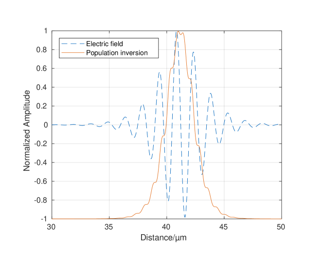
Figure 3: Simulation results from the self-induced transparency simulation setup, cf. Ziolkowski et al. [11], Fig. 2.

Listing 1 shows the complete Python code required to set up and run the SIT example. After the mbsolve libraries are imported, the script creates two materials, one of which features a simple two-level quantum mechanical description. The device to be simulated contains three regions, where vacuum is assigned to the first and third regions, and the active region is put in the middle. Initially, all quantum mechanical systems are inverted, which is represented by the initial density matrix rho_init. The scenario specifies 32768 spatial grid points, and that the simulation is run for $200\text{\,}\mathrm{fs}$. Furthermore, two records are added that request the recording of the population inversion and the electric field, respectively. Both quantities are to be sampled using a time interval of $2.5\text{\,}\mathrm{fs}$ over the complete spatial domain. Also, a source, which represents a sech pulse at the left end of the device, is added to the scenario. Finally, the solver is created and runs the simulation. On a recent quad-core desktop computer this simulation should be processed in less than 20 seconds. The results are passed to the writer, which stores the data in a HDF5 file.

Listing 1: Python script for the self-induced transparency (SIT) setup, cf. tools/python/ziolkowski1995.py in the mbsolve repository [64].

⬇

# import mbsolve libraries

import mbsolve.lib as mb

import mbsolve.solvercpu

import mbsolve.writerhdf5

# vacuum

mat_vac = mb.material("Vacuum")

mb.material.add_to_library(mat_vac)

# simple two-level quantum mechanical description

# params: particle density, transition frequency,

# transition dipole length,

# scattering rate gamma_1, dephasing rate gamma_2,

# equilibrium population inversion w_0

qm = mb.qm_desc_2lvl(1e24, 2 * math.pi * 2e14, 6.24e-11, 1.0e10, 1.0e10,

-1.0)

# Ziolkowski active region material

mat_ar = mb.material("AR_Ziolkowski", qm)

mb.material.add_to_library(mat_ar)

# Ziolkowski device setup

dev = mb.device("Ziolkowski")

# params of each region: name, material, x_start, x_end

dev.add_region(mb.region("Vacuum␣left", mat_vac, 0, 7.5e-6))

dev.add_region(mb.region("Active␣region", mat_ar, 7.5e-6, 142.5e-6))

dev.add_region(mb.region("Vacuum␣right", mat_vac, 142.5e-6, 150e-6))

# initial density matrix

# params: lower level rho_11 fully populated, upper level rho_22 empty

# vector with coherence terms not set in params, zero by default

rho_init = mb.qm_operator([ 1, 0 ])

# scenario

ic_d = mb.ic_density_const(rho_init)

ic_e = mb.ic_field_const(0.0)

sce = mb.scenario("Basic", 32768, 200e-15, ic_d, ic_e)

# record electric field and population inversion in 2.5fs intervals

sce.add_record(mb.record("inv12", 2.5e-15))

sce.add_record(mb.record("e", 2.5e-15))

# add source

sce.add_source(mb.sech_pulse("sech", 0.0, mb.source.hard_source,

4.2186e9, 2e14, 10, 2e14))

# run solver (advanced FDTD implementation + approach by Bidegaray 2001)

sol = mb.solver.create_instance("cpu-fdtd-red-2lvl-reg-cayley", dev,

sce)

sol.run()

# write results

wri = mb.writer.create_instance("hdf5")

outfile = dev.get_name() + "_" + sce.get_name() + "." +

wri.get_extension()

results = sol.get_results()

wri.write(outfile, sol.get_results(), dev, sce)

4.2 Pulse propagation in a V-type three-level system

Using Maxwell-Bloch simulations, Song et al. [51] investigated a setup that is conceptually similar to the SIT example, the major difference being the active region. Here, atomic rubidium was modeled as a three-level quantum mechanical system. While the work mainly focused on the propagation of few-cycle pulses, it also contains the temporal simulation of a single three-level system that is driven by a pulse (cf. [51], Fig. 3). This case can be reproduced by solving the Lindblad master equation alone.

In Listing 2, the creation of a device and a scenario for this setup is given. Since a three-level system is considered here, we have to use the complete quantum mechanical description including the operators and superoperator. In this example, the device contains only one region of zero length. This is the first indication that the simulation does not consider any spatial dimensions. The second indication is the number of grid points, which is passed to the scenario constructor. Here, the number of spatial grid points is set to 1, whereas the 10000 temporal grid points are specified. Similar to the SIT setup, records and sources can be added, although it only makes sense to add them at the position of the single grid point. It should be noted that for a low number of spatial grid points parallelization of the calculation does not make sense. Fortunately, it is not needed here as this example will complete within seconds on a recent desktop computer (using only one core).

Listing 2: Code snippet of the Python script that reproduces the three-level driven quantum mechanical system in [51], cf. tools/python/song2005.py in the mbsolve repository [64].

⬇

# Hamiltonian

# (diagonal qm operator, vector for off-diagonal terms omitted)

energies = [ 0, 2.3717e15 * mb.HBAR, 2.4165e15 * mb.HBAR ]

H = mb.qm_operator(energies)

# dipole moment operator (qm operator with off-diagonal terms)

dipoles = [ -mb.E0 * 9.2374e-11, -mb.E0 * 9.2374e-11 * math.sqrt(2), 0]

u = mb.qm_operator([ 0, 0, 0 ], dipoles)

# relaxation superoperator

rate = 1e10

# scattering rate matrix R

rates = [ [ 0, rate, rate ], [ rate, 0, rate ], [ rate, rate, 0 ] ]

# pure dephasing rates are zero in this example

pure_deph = [ 0, 0, 0 ]

relax_sop = mb.qm_lindblad_relaxation(rates, pure_deph)

# initial density matrix

rho_init = mb.qm_operator([ 1, 0, 0 ])

# quantum mechanical description

qm = mb.qm_description(6e24, H, u, relax_sop)

mat_ar = mb.material("AR_Song", qm)

mb.material.add_to_library(mat_ar)

# Song setup

dev = mb.device("Song")

dev.add_region(mb.region("Active␣region␣(single␣point)", mat_ar, 0, 0))

# scenario

ic_d = mb.ic_density_const(rho_init)

ic_e = mb.ic_field_const(0.0)

ic_m = mb.ic_field_const(0.0)

sce = mb.scenario("Basic", 1, 80e-15, ic_d, ic_e, ic_m, 10000)

sce.add_record(mb.record("e", 0.0, 0.0))

sce.add_record(mb.record("d11", mb.record.density, 1, 1, 0.0, 0.0))

sce.add_record(mb.record("d22", mb.record.density, 2, 2, 0.0, 0.0))

sce.add_record(mb.record("d33", mb.record.density, 3, 3, 0.0, 0.0))

# add source

sce.add_source(mb.sech_pulse("sech", 0.0, mb.source.hard_source,

3.5471e9, 3.8118e14, 17.248, 1.76/5e-15,

-math.pi/2))

4.3 Six-level anharmonic ladder system

In the work by Marskar and Österberg [16], two simulation examples are discussed. The first example is a variation of the SIT setup in [11], which we have already discussed above. The second example considers the propagation of a Gaussian pulse in a medium that is modeled as a six-level anharmonic ladder system (cf. [16], Fig. 4). In this system, the energy levels are given as

$$E_{n+1}=E_{n}+\hbar\omega_{0}[1-0.1(n-3)],$$ (28)

where $n\in[1;N-1]$, $N$ is the number of energy levels, and $\omega_{0}=$2\pi\text{\times}{10}^{13}\text{\,}{\mathrm{s}}^{-1}$$ is the transition frequency between the energy levels $E_{3}$ and $E_{4}$. For convenience, and without loss of generality, we set $E_{1}=0$ to zero.

From our perspective, this setup is no more than an variation of the previous examples. However, it gives us a nice opportunity to introduce the mbsolve-tool, which features different simulation examples written in C++. In fact, all examples discussed in this section can be started by specifying the setup name as well as an appropriate solver and writer as command line arguments. For example, the anharmonic ladder simulation can be started as

  $ mbsolve-tool -w hdf5 -m cpu-fdtd-red-6lvl-reg-cayley -d marskar2011-6lvl

Depending on the given setup name, the application creates the corresponding device and scenario, runs the specified solver, and uses the given writer to store the simulation results. Further command line arguments can be used to specify the number of spatial grid points and the simulation end time. This feature was extensively used during performance tests [41]. By default, 8192 spatial grid points and a simulation end time of $2\text{\,}\mathrm{ns}$ are used, resulting in a runtime of approximately two minutes on a recent quad-core desktop computer.

We note that in the command line entry above, the number of energy levels seems to be stated explicitly as part of the device name. Indeed, the name “marskar2011-6lvl” and the shortcut “marskar2011” refer to the original setup, but in fact any number $N\geq 2$ can be specified. This is a feature we added for performance comparisons of numerical methods, in which the performance is analyzed with respect to the number of energy levels (e.g., in [42, 43]). While the generalized example may not necessarily make sense from the modeling point of view, it represents a typical application example and hence constitutes a reasonable benchmark.

4.4 Quantum cascade laser frequency comb

Finally, we present the most complex and computationally demanding application example, as one simulation run required up to two hours on an AMD Ryzen Threadripper 2990WX machine using 16 cores. The quantum cascade laser frequency comb presented in [65] was modeled in previous work of our group [28], where the experimental results were reproduced with good agreement. Most input parameters were determined using prerequisite Schrödinger-Poisson and ensemble Monte Carlo simulations. Thereby, the number of empirical model parameters were reduced to a minimum.

Listing 3 shows how a similar simulation can be set up using the mbsolve software. First, the quantum mechanical description of the active region material is created. Apart from the five eigenenergies on the main diagonal, the Hamiltonian in this example has non-zero off-diagonal elements, which account for tunneling effects. All the elements are determined by a Schrödinger-Poisson simulation in tight-binding basis [25]. The dipole moment operator is less spectacular as it only contains one non-zero element, which is placed on the off-diagonal element that corresponds to the transition between upper and lower laser level. The scattering rates and dephasing rates are used to set up the Lindblad relaxation superoperator. The quantum mechanical description and the active region material are then created using the parameters from [28]. Then, semi-transparent mirror boundary conditions are created, with the reflectivity values $R_{1}=R_{2}=0.8$. The boundary conditions are subsequently used during the creation of the device, to which one region of the active region material is added. After that, the scenario is set up using the initial density matrix, in which only the upper laser level is populated. The electric field is initialized randomly to model stimulated emission, whereas the magnetic field is set to zero. Since this is the default in mbsolve, we do not need to specify this choice of initial conditions explicitly. Finally, a record that triggers the recording of the electrical field at the facet is added to the scenario.

Listing 3: Code snippet of the mbsolve-tool C++ application that reproduces the quantum cascade laser frequency comb simulation in [28], cf. mbsolve-tool/src/mbsolve-tool.cpp in the mbsolve repository [64].

⬇

/* quantum mechanical description of active region */

/* params: vector of main diagonal entries, followed by vector of

* off-diagonal entries */

mbsolve::qm_operator H(

{ 0.10103 * mbsolve::E0, 0.09677 * mbsolve::E0, 0.09720 * mbsolve::E0,

0.08129 * mbsolve::E0, 0.07633 * mbsolve::E0 },

{ 0.0, 1.2329e-3 * mbsolve::E0, -1.3447e-3 * mbsolve::E0,

0.0, 0.0, 0.0, 0.0, 0.0, 0.0, 0.0 });

mbsolve::qm_operator u(

{ 0.0, 0.0, 0.0, 0.0, 0.0 },

{ 0.0, 0.0, 0.0, 0.0, 0.0, -mbsolve::E0 * 4e-9, 0.0, 0.0, 0.0, 0.0 });

/* the scattering rate matrix R */

std::vector<std::vector<mbsolve::real> > scattering_rates = {

{ 0.0000000, 0.4947e12, 0.0974e12, 0.8116e12, 1.0410e12 },

{ 0.8245e12, 0.0000000, 0.1358e12, 0.6621e12, 1.1240e12 },

{ 0.0229e12, 0.0469e12, 0.0000000, 0.0794e12, 0.0357e12 },

{ 0.0047e12, 0.0029e12, 0.1252e12, 0.0000000, 0.2810e12 },

{ 0.0049e12, 0.0049e12, 0.1101e12, 0.4949e12, 0.0000000 }

};

mbsolve::real deph_inj_ull = 1.0/(0.6e-12);

mbsolve::real deph_xxx_xxx = 1.0/(1.0e-12);

/* the vector of pure dephasing rates */

std::vector<mbsolve::real> dephasing_rates =

{ 0, deph_inj_ull, deph_inj_ull, deph_xxx_xxx, deph_xxx_xxx,

deph_xxx_xxx, deph_xxx_xxx, deph_xxx_xxx, deph_xxx_xxx,

deph_xxx_xxx };

auto relax_sop = std::make_shared<mbsolve::qm_lindblad_relaxation>(

scattering_rates,

dephasing_rates);

auto qm = std::make_shared<mbsolve::qm_description>(5.6e21, H, u,

relax_sop);

auto mat_ar = std::make_shared<mbsolve::material>("AR", qm, 12.96, 0.9,

1100);

/* set up device with semi-transparent mirror boundary cond. */

auto bc =

std::make_shared<mbsolve::bc_field_reflectivity>(0.8, 0.8);

dev = std::make_shared<mbsolve::device>("tzenov2016", bc);

dev->add_region(std::make_shared<mbsolve::region>(

"Active␣region", mat_ar, 0, 5e-3));

/* initial density matrix (rho_33 is fully populated) */

mbsolve::qm_operator rho_init({ 0.0, 0.0, 1.0, 0.0, 0.0 });

/* basic scenario */

scen = std::make_shared<mbsolve::scenario>(

"basic", num_gridpoints, sim_endtime, rho_init);

scen->add_record(std::make_shared<mbsolve::record>(

"e0", mbsolve::record::electric, 1, 1, 0.0, 0.0));

After a solver has processed the device and scenario, the result data are written to a HDF5 file. At this point, we would like to discuss briefly the postprocessing of results. Typically, several tasks remain to be done after the solver has completed. In this case, the Fourier transform of the recorded electric field must be calculated and plotted. Naturally, this is beyond the scope of mbsolve and established software tools, such as MATLAB, Octave, or Python (with NumPy, SciPy, and Matplotlib), should be used. Examples for postprocessing MATLAB scripts can be found in tools/matlab in the mbsolve repository [64].

The simulation results (after postprocessing) are depicted in Fig. 4. While the spectrum of the electric field at the facet shows reasonable agreement with the experiment, there are features missing that the simulation in [28] could capture. We believe that this is due to the differences in the underlying simulation methods. While the method in this work does not invoke the RWA, it does not account for chromatic dispersion or diffusion processes due to spatial hole burning.

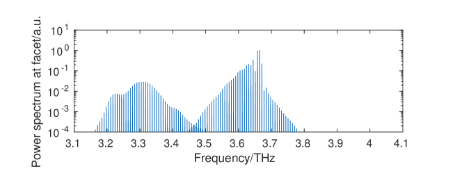
Figure 4: Power spectrum of the electric field recorded at the facet of the quantum cascade laser frequency comb. This simulation example bases on Tzenov et al. [28] (cf. Fig. 5c). For the corresponding experimental results cf. Burghoff et al. [65], Fig. 3b.

5 Conclusion

In this paper, we have presented mbsolve, an open-source solver tool for the Maxwell-Bloch equations. Here, we have focused on the one-dimensional case, which is suitable for e.g., modeling various types of optoelectronic devices such as QCLs, where the waveguide geometry allows a reduction of the model to one spatial dimension. Besides optoelectronic devices, the resulting equations can be applied to a variety of problems in which the plane-wave approximation is a reasonable assumption. Also, we have outlined the numerical treatment of the Maxwell-Bloch equations, focusing on methods that do not invoke the RWA/SVEA. Additionally, the methods are able to handle an arbitrary number of energy levels, i.e., the Lindblad equation is solved rather than the (two-level) optical Bloch equations.

The basic library of mbsolve provides a flexible and extensible framework to describe devices to be modeled, and simulation scenarios. On this basis, solvers can be written that implement different numerical methods and/or parallelization techniques. Similarly, writers can be implemented that export the simulation results to certain file formats. We have implemented and described two solvers that base on the FDTD method and use the OpenMP standard for parallelization, two algorithms for solving the Lindblad equation, and a writer for the HDF5 file format. The resulting source code is written in C++ and features automatically generated bindings for Python. It is open-source and can be compiled using most of the established C++ compilers on all major platforms. Alternatively, the mbsolve software can be installed in binary form using the conda package manager.

We have demonstrated the usage of our software with the help of four application examples, selected to cover different use cases. The first example features a two-level medium that can be described using a simplified version of the quantum mechanical description. The setup of the second simulation example can be considered a driven quantum mechanical system. In this simulation, there is no spatial coordinate, i.e., field propagation effects are not considered. The third example uses the generalized quantum mechanical description to handle the six-level medium. Finally, the last example is a simulation of an actual quantum cascade laser. This example is the most complex and computationally most demanding simulation.

Although the mbsolve software is already a helpful and reliable tool, several interesting issues are still unsolved, and potential optimization possibilities remain to be exploited. The discussion of numerical methods is ongoing and we hope that in the near future additional methods are implemented in the mbsolve project. Although the methods for the Lindblad equation seem to have more room for improvement, there are also promising alternative candidates for Maxwell’s equations (e.g., methods that use adaptive spatial grids). While we have focused on methods that avoid the RWA/SVEA, we note that those approximations are beneficial for several applications. In future work, a solver that uses a numerical method that invokes the RWA (such as the Risken-Nummedal scheme [66]) could be implemented to support these applications better. As to parallelization, the existing solvers are to be extended to distributed memory systems using Message Passing Interface (MPI) standard. Furthermore, offloading of calculations to graphics processing units (GPUs) is an intriguing possibility.

From the modeling point of view, the inclusion of dispersion in the electromagnetic properties will be the next step. While it is not exactly trivial to implement, it is bound to play a significant role in the modeling of optoelectronic devices (see e.g., [67]). Also, the implementation of alternative boundary conditions will extend the application range of mbsolve, e.g., to the simulation of ring cavities. Finally, in order to enable numerically efficient simulations in two or three spatial dimensions, an attractive strategy could be to integrate the mbsolve code for the Lindblad equation into an established and high-performance open-source electromagnetics simulation project, such as MEEP.

References

- [1] R. W. Boyd, Nonlinear Optics, 3rd Edition, Academic Press, 2008.
- [2] F. Bloch, Nuclear induction, Phys. Rev. 70 (1946) 460–474. doi:10.1103/PhysRev.70.460.
- [3] R. P. Feynman, F. L. Vernon, R. W. Hellwarth, Geometrical representation of the Schrödinger equation for solving maser problems, J. Appl. Phys. 28 (1) (1957) 49–52. doi:10.1063/1.1722572.
- [4] F. T. Arecchi, R. Bonifacio, Theory of optical maser amplifiers, IEEE J. Quantum Electron. 1 (4) (1965) 169–178. doi:10.1109/JQE.1965.1072212.
- [5] I. D. Abella, N. A. Kurnit, S. R. Hartmann, Photon echoes, Phys. Rev. 141 (1966) 391–406. doi:10.1103/PhysRev.141.391.
- [6] S. L. McCall, E. L. Hahn, Self-induced transparency by pulsed coherent light, Phys. Rev. Lett. 18 (1967) 908–911. doi:10.1103/PhysRevLett.18.908.
- [7] S. L. McCall, E. L. Hahn, Self-induced transparency, Phys. Rev. 183 (1969) 457–485. doi:10.1103/PhysRev.183.457.
- [8] F. T. Hioe, J. H. Eberly, -level coherence vector and higher conservation laws in quantum optics and quantum mechanics, Phys. Rev. Lett. 47 (12) (1981) 838–841. doi:10.1103/PhysRevLett.47.838.
- [9] L. V. Hau, S. E. Harris, Z. Dutton, C. H. Behroozi, Light speed reduction to 17 metres per second in an ultracold atomic gas, Nature 397 (6720) (1999) 594–598. doi:10.1038/17561.
- [10] C. Liu, Z. Dutton, C. H. Behroozi, L. V. Hau, Observation of coherent optical information storage in an atomic medium using halted light pulses, Nature 409 (6819) (2001) 490–493. doi:10.1038/35054017.
- [11] R. W. Ziolkowski, J. M. Arnold, D. M. Gogny, Ultrafast pulse interactions with two-level atoms, Phys. Rev. A 52 (4) (1995) 3082–3094. doi:10.1103/PhysRevA.52.3082.
- [12] W. Cartar, J. Mørk, S. Hughes, Self-consistent Maxwell-Bloch model of quantum-dot photonic-crystal-cavity lasers, Phys. Rev. A 96 (2) (2017) 023859. doi:10.1103/PhysRevA.96.023859.
- [13] P. Gładysz, Piotr Wcisło, K. Słowik, Propagation of optically tunable coherent radiation in a medium of asymmetric molecules, Sci. Rep. 10 (1) (2020) 17615. doi:10.1038/s41598-020-74569-w.
- [14] G. Slavcheva, J. M. Arnold, I. Wallace, R. W. Ziolkowski, Coupled Maxwell-pseudospin equations for investigation of self-induced transparency effects in a degenerate three-level quantum system in two dimensions: Finite-difference time-domain study, Phys. Rev. A 66 (6) (2002) 63418. doi:10.1103/PhysRevA.66.063418.
- [15] M. Sukharev, A. Nitzan, Numerical studies of the interaction of an atomic sample with the electromagnetic field in two dimensions, Phys. Rev. A 84 (4) (2011) 043802. doi:10.1103/PhysRevA.84.043802.
- [16] R. Marskar, U. Österberg, Multilevel Maxwell-Bloch simulations in inhomogeneously broadened media, Opt. Express 19 (18) (2011) 16784–16796. doi:10.1364/OE.19.016784.
- [17] C. Jirauschek, M. Riesch, P. Tzenov, Optoelectronic device simulations based on macroscopic Maxwell–Bloch equations, Adv. Theor. Simul. 2 (8) (2019) 1900018. doi:10.1002/adts.201900018.
- [18] R. F. Kazarinov, R. A. Suris, Possibility of the amplification of electromagnetic waves in a semiconductor with a superlattice, Sov. Phys. Semicond. 5 (4) (1971) 797–800.
- [19] J. Faist, F. Capasso, D. L. Sivco, C. Sirtori, A. L. Hutchinson, A. Y. Cho, Quantum cascade laser, Science 264 (5158) (1994) 553–556. doi:10.1126/science.264.5158.553.
- [20] C. Y. Wang, L. Diehl, A. Gordon, C. Jirauschek, F. X. Kärtner, A. Belyanin, D. Bour, S. Corzine, G. Höfler, M. Troccoli, J. Faist, F. Capasso, Coherent instabilities in a semiconductor laser with fast gain recovery, Phys. Rev. A 75 (3) (2007) 031802. doi:10.1103/PhysRevA.75.031802.
- [21] C. R. Menyuk, M. A. Talukder, Self-induced transparency modelocking of quantum cascade lasers, Phys. Rev. Lett. 102 (2) (2009) 023903. doi:10.1103/PhysRevLett.102.023903.
- [22] H. Choi, V.-M. Gkortsas, L. Diehl, D. Bour, S. Corzine, J. Zhu, G. Höfler, F. Capasso, F. X. Kärtner, T. B. Norris, Ultrafast Rabi flopping and coherent pulse propagation in a quantum cascade laser, Nat. Photonics 4 (10) (2010) 706–710. doi:10.1038/nphoton.2010.205.
- [23] V.-M. Gkortsas, C. Y. Wang, L. Kuznetsova, L. Diehl, A. Gordon, C. Jirauschek, M. A. Belkin, A. Belyanin, F. Capasso, F. X. Kärtner, Dynamics of actively mode-locked quantum cascade lasers, Opt. Express 18 (13) (2010) 13616–13630. doi:10.1364/OE.18.013616.
- [24] J. R. Freeman, J. Maysonnave, S. Khanna, E. H. Linfield, A. G. Davies, S. Dhillon, J. Tignon, Laser-seeding dynamics with few-cycle pulses: Maxwell-Bloch finite-difference time-domain simulations of terahertz quantum cascade lasers, Phys. Rev. A 87 (6) (2013) 063817. doi:10.1103/PhysRevA.87.063817.
- [25] C. Jirauschek, T. Kubis, Modeling techniques for quantum cascade lasers, Appl. Phys. Rev. 1 (2014) 011307. doi:10.1063/1.4863665.
- [26] M. A. Talukder, C. R. Menyuk, Quantum coherent saturable absorption for mid-infrared ultra-short pulses, Opt. Express 22 (13) (2014) 15608–15617. doi:10.1364/OE.22.015608.
- [27] Y. Wang, A. Belyanin, Active mode-locking of mid-infrared quantum cascade lasers with short gain recovery time, Opt. Express 23 (4) (2015) 4173–4185. doi:10.1364/OE.23.004173.
- [28] P. Tzenov, D. Burghoff, Q. Hu, C. Jirauschek, Time domain modeling of terahertz quantum cascade lasers for frequency comb generation, Opt. Express 24 (20) (2016) 23232–23247. doi:10.1364/OE.24.023232.
- [29] N. N. Vuković, J. Radovanović, V. Milanović, D. L. Boiko, Low-threshold RNGH instabilities in quantum cascade lasers, IEEE J. Sel. Top. Quant. 23 (6) (2017) 1–16. doi:10.1109/JSTQE.2017.2699139.
- [30] P. Tzenov, I. Babushkin, R. Arkhipov, M. Arkhipov, N. N. Rosanov, U. Morgner, C. Jirauschek, Passive and hybrid mode locking in multi-section terahertz quantum cascade lasers, New J. Phys. 20 (5) (2018) 053055. doi:10.1088/1367-2630/aac12a.
- [31] L. Columbo, S. Barbieri, C. Sirtori, M. Brambilla, Dynamics of a broad-band quantum cascade laser: from chaos to coherent dynamics and mode-locking, Opt. Express 26 (3) (2018) 2829–2847. doi:10.1364/OE.26.002829.
- [32] P. K. Nielsen, H. Thyrrestrup, J. Mørk, B. Tromborg, Numerical investigation of electromagnetically induced transparency in a quantum dot structure, Opt. Express 15 (10) (2007) 6396–6408. doi:10.1364/OE.15.006396.
- [33] N. Majer, K. Lüdge, E. Schöll, Cascading enables ultrafast gain recovery dynamics of quantum dot semiconductor optical amplifiers, Phys. Rev. B 82 (23) (2010) 235301. doi:10.1103/PhysRevB.82.235301.
- [34] G. Slavcheva, M. Koleva, A. Rastelli, Ultrafast pulse phase shifts in a charged-quantum-dot–micropillar system, Phys. Rev. B 99 (11) (2019) 115433. doi:10.1103/PhysRevB.99.115433.
- [35] M. Riesch, P. Tzenov, C. Jirauschek, Dynamic simulations of quantum cascade lasers beyond the rotating wave approximation, in: 2018 2nd URSI Atlantic Radio Science Meeting (AT-RASC), IEEE, Piscataway, NJ, 2018. doi:10.23919/URSI-AT-RASC.2018.8471596.
- [36] M. Riesch, J. H. Abundis-Patino, P. Tzenov, C. Jirauschek, Efficient simulation of the quantum cascade laser dynamics beyond the rotating wave approximation, in: Proceedings of the International Quantum Cascade Laser School and Workshop (IQCLSW) 2018, 2018.
- [37] B. Bidégaray, A. Bourgeade, D. Reignier, Introducing physical relaxation terms in Bloch equations, J. Comput. Phys. 170 (2) (2001) 603–613.
- [38] B. Bidégaray, Time discretizations for Maxwell-Bloch equations, Numer. Methods Partial Differ. Equ. 19 (3) (2003) 284–300. doi:10.1002/num.10046.
- [39] O. Saut, A. Bourgeade, Numerical methods for the bidimensional Maxwell–Bloch equations in nonlinear crystals, J. Comput. Phys. 213 (2) (2006) 823–843. doi:10.1016/j.jcp.2005.09.003.
- [40] A. Deinega, T. Seideman, Self-interaction-free approaches for self-consistent solution of the Maxwell-Liouville equations, Phys. Rev. A 89 (2) (2014) 022501.
- [41] M. Riesch, N. Tchipev, S. Senninger, H.-J. Bungartz, C. Jirauschek, Performance evaluation of numerical methods for the Maxwell–Liouville–von Neumann equations, Opt. Quant. Electron. 50 (2) (2018) 112. doi:10.1007/s11082-018-1377-4.
- [42] M. Riesch, C. Jirauschek, Completely positive trace preserving numerical methods for long-term generalized Maxwell-Bloch simulations, in: Lasers and Electro-Optics Europe & European Quantum Electronics Conference (CLEO/Europe-EQEC), 2019 Conference on, IEEE, Piscataway, NJ, 2019. doi:10.1109/CLEOE-EQEC.2019.8873263.
- [43] M. Riesch, A. Pikl, C. Jirauschek, Completely positive trace preserving methods for the Lindblad equation, in: Numerical Simulation of Optoelectronic Devices (NUSOD), 2020 International Conference on, IEEE, Piscataway, NJ, 2020. doi:10.1109/NUSOD49422.2020.9217670.
- [44] Kintechlab, Electromagnetic template library, \urlhttp://fdtd.kintechlab.com/en/start (2018).
- [45] J. Javaloyes, S. Balle, Freetwm: a simulation tool for semiconductor lasers, \urlhttps://onl.uib.eu/Softwares/Freetwm/ (2018).
- [46] A. F. Oskooi, D. Roundy, M. Ibanescu, P. Bermel, J. D. Joannopoulos, S. G. Johnson, Meep: A flexible free-software package for electromagnetic simulations by the FDTD method, Comput. Phys. Commun. 181 (3) (2010) 687–702. doi:10.1016/j.cpc.2009.11.008.
- [47] M. Riesch, N. Tchipev, H.-J. Bungartz, C. Jirauschek, Numerical simulation of the quantum cascade laser dynamics on parallel architectures, in: Proceedings of the Platform for Advanced Scientific Computing Conference, ACM, New York, NY, 2019, pp. 5:1–5:8. doi:10.1145/3324989.3325715.
- [48] F. Wang, V. Pistore, M. Riesch, H. Nong, P.-B. Vigneron, R. Colombelli, O. Parillaud, J. Mangeney, J. Tignon, C. Jirauschek, S. S. Dhillon, Ultrafast response of active and self-starting harmonic modelocked THz laser, Light Sci. Appl. 9 (1) (2020) 51. doi:10.1038/s41377-020-0288-x.
- [49] F. P. Mezzapesa, K. Garrasi, J. Schmidt, L. Salemi, V. Pistore, L. Li, A. G. Davies, E. H. Linfield, M. Riesch, C. Jirauschek, T. Carey, F. Torrisi, A. C. Ferrari, M. S. Vitiello, Terahertz frequency combs exploiting an on-chip, solution processed, graphene-quantum cascade laser coupled-cavity, ACS Photonics 7 (12) (2020) 3489–3498. doi:10.1021/acsphotonics.0c01523.
- [50] A. E. Siegman, Lasers, University Science Books, Mill Valley, California, 1986.
- [51] X. Song, S. Gong, Z. Xu, Propagation of a few-cycle laser pulse in a V-type three-level system, Opt. Spectrosc. 99 (4) (2005) 517–521. doi:10.1134/1.2113361.
- [52] A. Taflove, S. C. Hagness, Computational Electrodynamics: The Finite-Difference Time-Domain Method, Artech House, 2005.
- [53] M. Riesch, C. Jirauschek, Analyzing the positivity preservation of numerical methods for the Liouville-von Neumann equation, J. Comput. Phys. 390 (2019) 290–296. doi:10.1016/j.jcp.2019.04.006.
- [54] M. Riesch, C. Jirauschek, Numerical method for the Maxwell-Liouville-von Neumann equations using efficient matrix exponential computations, arxiv:1710.09799.
- [55] M. Riesch, N. Tchipev, H.-J. Bungartz, C. Jirauschek, Solving the Maxwell-Bloch equations efficiently on parallel architectures, in: Lasers and Electro-Optics Europe & European Quantum Electronics Conference (CLEO/Europe-EQEC), 2017 Conference on, IEEE, Piscataway, NJ, 2017. doi:10.1109/CLEOE-EQEC.2017.8087734.
- [56] M. Riesch, T. D. Nguyen, C. Jirauschek, bertha: Project skeleton for scientific software, PLOS ONE 15 (3) (2020) e0230557. doi:10.1371/journal.pone.0230557.
- [57] M. Riesch, qclsip: The Quantum Cascade Laser Stock Image Project (Jan. 2019). doi:10.5281/zenodo.2641239.
- [58] H.-P. Breuer, F. Petruccione, The Theory of Open Quantum Systems, Oxford University Press, Oxford, 2002.
- [59] G. Lindblad, On the generators of quantum dynamical semigroups, Commun. Math. Phys. 48 (2) (1976) 119–130. doi:10.1007/BF01608499.
- [60] V. Gorini, A. Kossakowski, E. C. G. Sudarshan, Completely positive dynamical semigroups of -level systems, J. Math. Phys. 17 (5) (1976) 821–825. doi:10.1063/1.522979.
- [61] S. G. Schirmer, A. I. Solomon, Constraints on relaxation rates for -level quantum systems, Phys. Rev. A 70 (2004) 022107. doi:10.1103/PhysRevA.70.022107.
- [62] D. K. L. Oi, S. G. Schirmer, Limits on the decay rate of quantum coherence and correlation, Phys. Rev. A 86 (2012) 012121. doi:10.1103/PhysRevA.86.012121.
- [63] mbsolve documentation on GitHub Pages, \urlhttps://mriesch-tum.github.io/mbsolve (2020).
- [64] M. Riesch, C. Jirauschek, mbsolve: An open-source solver tool for the Maxwell-Bloch equations, \urlhttps://github.com/mriesch-tum/mbsolve (Jul. 2017).
- [65] D. Burghoff, T.-Y. Kao, N. Han, C. W. I. Chan, X. Cai, Y. Yang, D. J. Hayton, J.-R. Gao, J. L. Reno, Q. Hu, Terahertz laser frequency combs, Nature Photon. 8 (6) (2014) 462–467. doi:10.1038/nphoton.2014.85.
- [66] H. Risken, K. Nummedal, Self-pulsing in lasers, J. Appl. Phys. 39 (10) (1968) 4662–4672. doi:10.1063/1.1655817.
- [67] M. Singleton, P. Jouy, M. Beck, J. Faist, Evidence of linear chirp in mid-infrared quantum cascade lasers, Optica 5 (8) (2018) 948–953. doi:10.1364/OPTICA.5.000948.