Earths in Other Solar Systems N-body simulations: the Role of Orbital Damping in Reproducing the Kepler Planetary Systems

Abstract

The population of exoplanetary systems detected by Kepler provides opportunities to refine our understanding of planet formation. Unraveling the conditions needed to produce the observed exoplanet systems will allow us to make informed predictions as to where habitable worlds exist within the galaxy. In this paper, we examine using N-body simulations how the properties of planetary systems are determined during the final stages of assembly, when planets accrete from embryos and planetesimals. While accretion is a chaotic process, trends emerge allowing certain features of an ensemble of planetary systems to provide a memory of the initial distribution of solid mass around a star prior to accretion. We also use EPOS, the Exoplanet Population Observation Simulator, to account for detection biases and show that different accretion scenarios can be distinguished from observations of the Kepler systems. We show that the period of the innermost planet, the ratio of orbital periods of adjacent planets, and masses of the planets are determined by the total mass and radial distribution of embryos and planetesimals at the beginning of accretion. In general, some amount of orbital damping, either via planetesimals or gas, during accretion is needed to match the whole population of exoplanets. Surprisingly, all simulated planetary systems have planets that are similar in size, showing that the "peas in a pod" pattern can be consistent with both a giant impact scenario and a planet migration scenario. The inclusion of material at distances larger than what Kepler observes ($>1$ au) has a profound impact on the observed planetary architectures, and thus on the formation and delivery of volatiles to possible habitable worlds.

1 Introduction

Terrestrial planets form through the piece-wise collisional aggregation of solids spanning many orders of magnitude in size, beginning with micron-sized grains and continuing upward. The final stages of growth involve the accretion of swarms of planetesimals and embryos, bodies measuring hundreds to thousands of kilometers across. It is at these sizes where gravitational interactions lead to changes in the paths of these bodies around their central star, shifting them from the roughly circular orbits they develop within a gaseous protoplanetary disk, to more eccentric, crossing orbits, that result in collisions and thus growth. As protoplanets grow larger in this manner, the gravitational interactions work to space out the larger surviving bodies, isolating them from one another as the initial building blocks are largely cleared by further accretion, scattering out of the system, or collisions with the central star. This leaves behind a fairly stable system of planets, with a small amount of leftover primordial bodies (e.g. Raymond et al., 2014).

One possible outcome of this evolution is seen in the Solar System today, with planets orbiting at relatively large separations and with populations of small bodies within the asteroid belt, Kuiper Belt, and Oort Cloud. How the Solar System achieved this structure has been the focus of a number of studies that used N-body codes to simulate the final stages of planetary growth, tracking how a distribution of embryos and planetesimals interact and grow over time (e.g. Wetherill, 1994; Chambers & Wetherill, 1998; Chambers, 2001; Raymond et al., 2004, 2005, 2006, 2009; O’Brien et al., 2006, 2014; Bond et al., 2010a, b; Carter-Bond et al., 2012; Fischer & Ciesla, 2014; Walsh et al., 2011; Quintana et al., 2007; Quintana & Lissauer, 2014; Izidoro et al., 2013, 2014). The success of these models in understanding the final stages of planet formation has largely been evaluated by their ability to reproduce the properties of the Solar System. That is, key dynamical features (such as the mass of the asteroid belt, the angular momentum of the planets, their mass distribution, the low mass of Mars, and the timing of the last accretion event of the Earth) have been used to constrain the orbital properties of Jupiter and Saturn during terrestrial planet formation (O’Brien et al., 2006; Raymond et al., 2009), the radial distribution of mass of the planetesimals and embryos (Raymond et al., 2006), or the extent to which Jupiter migrated while the solar nebula was still present (Walsh et al., 2011).

These studies have also found that similar initial conditions can yield very different final planetary systems (e.g. Lissauer, 2007; Fischer & Ciesla, 2014). The chaotic nature of the final assembly phase presents a challenge when comparing our Solar System to the model outcomes. That is, it cannot be said with certainty whether our inability to simultaneously match all of the properties of the Solar System is due to the stochastic nature of the process and infinite number of possible outcomes that could be produced or if the initial conditions used in the models differ from those of reality.

While comparisons to the Solar System is a natural starting point to understand this stage of evolution, the discovery of thousands of exoplanetary systems has shown that our planetary system represents just one possible outcome of the planet formation process (e.g. Batalha, 2014). The large number of systems discovered now allows us to identify general trends and relationships between key properties that arise during planetary assembly. Thus, these systems provide a new opportunity to test our understanding of the final stages of planet formation by investigating how well our models reproduce general trends in observed exoplanet systems.

Here we report on our study that explores how the key properties of planetary systems relate back to the initial conditions when planetary accretion begins and what conditions were necessary to produce the final architectures of the planetary systems found around sun-like stars. Our goal is not to define or identify the best, single set of conditions that will reproduce the known planetary systems, but instead, to understand the connections and relationships between initial conditions that are responsible for defining the properties of the systems that we see today as a means of understanding formation pathways, and the bulk properties, for those planets (Apai et al., 2019).

Our approach here is to build a statistical framework in which we can model the outcomes of various planet formation scenarios and evaluate them against the known systems of exoplanets. Hansen & Murray (2013) carried out an initial study with these goals, arguing that the known Kepler systems could have formed if the final stages of assembly began with a massive disk of planetesimals concentrated within $\sim$1 au of their host stars. In particular, the distributions of orbital period and planet radius, as well as the relative frequencies of observed multi-planet systems produced in the models were consistent with those real systems that had been detected. Subsequent studies have corroborated and expanded on these results, focusing on the dynamical effects of residual gas in these simulations (Dawson et al., 2015, 2016) and explaining the apparent excess of single-transiting systems (Moriarty & Ballard, 2016).

Currently, the number of Kepler planet candidates has grown to over four thousand (Thompson et al., 2017) and the survey detection efficiency has been thoroughly characterized (e.g. Burke et al., 2015; Christiansen et al., 2016), providing a more robust set of data to describe actual planetary properties to which model systems can be compared to. We explore a wide range of parameter space, and generate a large number of model planetary systems in order to understand the distribution of outcomes possible for a given range of parameters. We then evaluate how well the distribution of planetary properties produced by these initial conditions compares to the Kepler dataset using the Exoplanet Population Observation Simulator (epos, Mulders et al., 2018, 2019). Again, we do not expect to identify a single set of parameters or scenarios that describes the formation of all known planetary systems; instead, we are evaluating whether particular signposts of the imprints of the initial conditions and process of planetary accretion can be identified within the data sets. Success would then inform us of the formation histories of these planets. In the next section, we describe the various sets of initial conditions and dynamical effects we considered in our simulations. The results of our simulations, which are part of the Genesis database of the Earths in Other Solar Systems project, are presented in Section 3. We compare the model results to the Kepler system using version 3.0 of the new epos tool in Section 4 to evaluate how well our models and assumptions about the final stages of planet formation match the real planetary systems that have been identified to date. We conclude with a discussion and outline of future work.

2 Dynamical Scenarios

In all of our simulations, we follow previous work by assuming the distribution of solids around a solar mass central star follows a power law given by a surface density $\sigma=\sigma_{o}\left(\frac{r}{\mathrm{1~{}au}}\right)^{-p}$, where $\sigma_{o}$ is the surface density at a semimajor axis of $r=1$ au with index $p$. This prescription defines how much mass is available to build planets and how radially concentrated it is with respect to the star. Some fraction of this mass, $f_{e}$, is assumed to be present in the form of embryos which interact through gravitational interactions with all other bodies in the system. The remaining fraction of solids, $f_{p}=1-f_{e}$, is taken to be present as planetesimals, which are smaller, less massive objects that interact gravitationally with the embryos but not with each other (a common computational simplification for these type of simulations). All of these bodies are then taken to be distributed across an annulus ranging from an inner radius, $a_{min}$, to an outer radius $a_{max}$, beyond which it is assumed no other solids are present.

In all cases, we assume that embryos are spaced an average of $\Delta$=7.5 mutual Hill radii apart, and thus have initial masses and semi-major axes defined by the relations in Kokubo & Ida (2000). For surface density slopes smaller than $p=2$, embryo mass increases with semi-major axis. Following Hansen & Murray (2013), the embryos are placed on initial orbits that are nearly circular, with eccentricities randomly assigned values between 0 and 0.001, and orbital inclinations are randomly assigned from 0 to 2^∘. The orientations of the orbits and the initial location of each body on it is determined from a uniform distribution to define the final set of orbital parameters. The initial orbital parameters of the planetesimals are defined in a similar manner, although in their case the individual planetesimal mass is fixed and semimajor axes are chosen so that their distribution follows the surface density profile. For the purposes of calculating the radii of the bodies of interest, we assume a density of $\rho$=3 g cm^-3. The inner edge of the simulations is set to half the semi-major axis of the innermost body at the start of the simulations, and the timestep is set to 1/20 of the orbital period at the cutoff distance. Bodies that pass interior to this cutoff distance are removed from the simulation.

Each of the simulations we perform is initialized by defining the parameters described above ($\sigma_{o}$, $p$, $f_{e}$, $a_{min}$, and $a_{max}$), and for each set of parameters many individual simulations are run with randomization of the orbital parameters as described above. We refer to each of these as a Run Set. The parameter values for all of the runs we consider here are listed in Table 1. Figure 1 also shows how the initial conditions compare across the various Run Sets, comparing and contrasting the initial radial distribution of the embryos and their masses. Below we describe the broad categories of simulations that we performed.

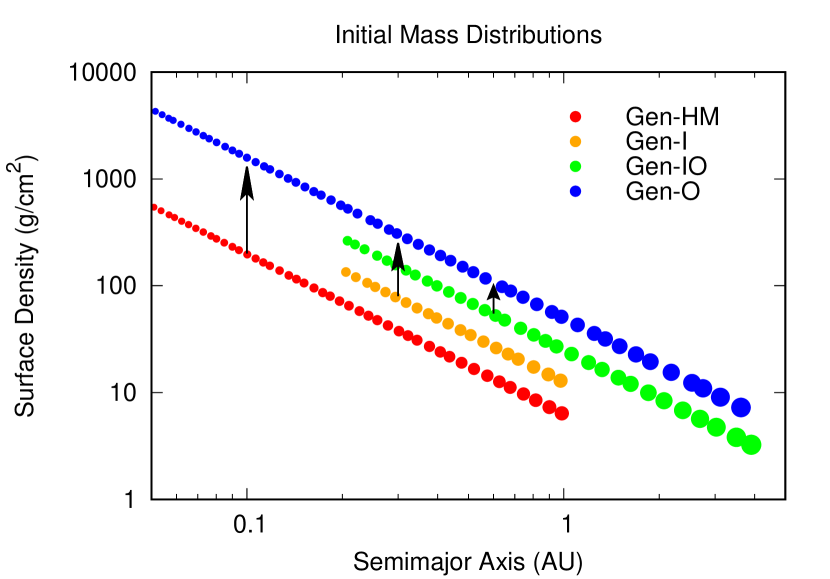
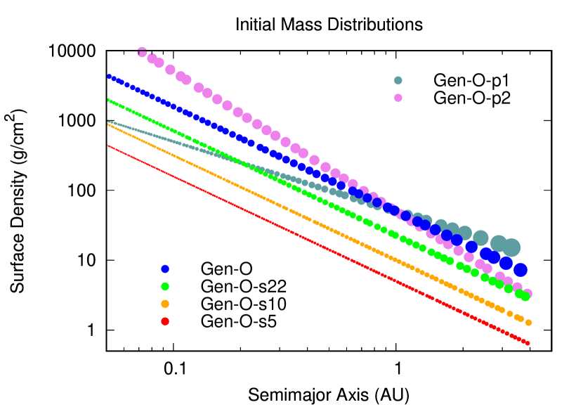
Figure 1: Starting surface density distribution for simulations with different initial conditions. Symbol size is proportional to embryo radius (assuming a constant density). The top panel shows simulations with different inner and outer radii, vertically offset for clarity. The bottom panel shows simulations with different surface density normalization factors and exponents.

Table 1: Key parameters for the different sets of runs that we performed. Values not shown here that were held constant across all runs are $M_{star}$ = 1 $\mathrm{M_{\odot}}$, the initial embryo spacing $\Delta$ = 7.5 mutual Hill radii, embryo and planetesimal density $\rho$ = 3 $\mathrm{g/cm^{3}}$, and initial eccentricity and inclination $e_{o}$ = 0.001 and $i_{o}$ = 2^o. The parameter values that were varied from the base model Gen-HM are denoted in bold face.

Run Name	$\sigma_{o}\ (\mathrm{g/cm^{2}})$	$p$	$a_{min}$ (au)	$a_{max}$ (au)	$a_{min,gas}$ (au)	$f_{emb}$	$N_{emb}$	$N_{ptsml}$	$N_{run}$
Gen-HM	50.00	1.50	0.05	1.00	n/a	1.00	45	0	50
Gen-P	50.00	1.50	0.05	1.00	n/a	0.75	51	1027	8
Gen-I	50.00	1.50	0.20	1.00	n/a	1.00	20	0	50
Gen-P-I	50.00	1.50	0.20	1.00	n/a	0.75	23	733	8
Gen-IO	50.00	1.50	0.20	4.00	n/a	1.00	32	0	50
Gen-P-IO	50.00	1.50	0.20	4.00	n/a	0.75	36	2055	8
Gen-O	50.00	1.50	0.05	4.00	n/a	1.00	56	0	50
Gen-O-p1	50.00	1.00	0.05	4.00	n/a	1.00	79	0	50
Gen-O-p2	50.00	2.00	0.05	4.00	n/a	1.00	44	0	50
Gen-O-s22	22.50	1.50	0.05	4.00	n/a	1.00	84	0	50
Gen-O-s10	10.00	1.50	0.05	4.00	n/a	1.00	126	0	50
Gen-O-s5	5.00	1.50	0.05	4.00	n/a	1.00	178	0	50
Gen-M-s50	50.00	1.50	0.05	10.00	0.05	1.00	62	0	50
Gen-M-s22	22.50	1.50	0.05	10.00	0.05	1.00	93	0	50
Gen-M-s10	10.00	1.50	0.05	10.00	0.05	1.00	139	0	50

2.1 Embryo-only

We performed several sets of simulations that consisted only of massive embryos ($f_{e}$=1) based on the initial conditions used in Hansen & Murray (2013) that were found to reproduce the broad properties of planetary systems in terms of planet radii, orbital periods, and multi-planet frequency in the Kepler catalog at the time. The nominal case (which we refer to as Gen-HM) is chosen to approximately reproduce their simulations, with surface mass density profile exponent $p$=3/2, normalization factor $\sigma_{o}=50\ \mathrm{g/cm^{2}}$ at 1 au, and embryos distributed between $a_{min}$ of 0.05 au and $a_{max}$ of 1 au. This gives 45 total embryos, with a total mass of 19 M_⨁ (in comparison, Hansen & Murray (2013) had 32-38 embryos and 20 M_⨁, likely due to a larger spacing between embryos). In addition to the nominal case, we systematically explored a number of other initial conditions, varying the radial range over which building blocks were distributed ($a_{min}$ - $a_{max}$, simulations Gen-I, Gen-IO, and Gen-O), the normalized surface density $\sigma_{o}$ at 1 au (Gen-O-s22, Gen-O-s10, Gen-O-s5), and the exponent $p$ of the power law that describes how the mass is distributed with radius (Gen-O-p1, Gen-O-p2. The surface density is a factor of five higher than what is needed to produce the terrestrial planets in the solar system (e.g. Raymond et al., 2006). Most simulations were carried out for 10 Myr, though we also ran many for longer periods of time (up to 80 Myr) to explore how planetary system structure varies over these longer timescales. The orbital evolution simulations were performed using the SWIFTER version of the SyMBA integrator (Duncan et al., 1998), which handles close encounters and mergers. We assume that all collisions result in perfect mergers. Including fragmentation in the simulations would prolong the time-scale for planetary accretion, but generally results in similar planet planetary system properties as most collisional products are re-accreted on the same planet (Chambers, 2013).

2.2 Planetesimals and Embryos

We also performed sets of simulations with a population of planetesimals distributed among the embryos (Gen-P, Gen-P-I, and Gen-P-IO). These small bodies have been shown to damp down the inclinations and eccentricities of forming planets through dynamical friction (e.g., Wetherill & Stewart, 1993; O’Brien et al., 2006). In these cases, we used the same total mass of solid materials as for our embryo-only cases, but distributed it with 75% being present as embryos initially ($f_{emb}=0.75$) and the remaining 25% initially being contained in planetesimals. In our Gen-P case, which follows our nominal model, the planetesimal mass is distributed as 1000 distinct bodies, giving an individual planetesimal mass that is $\sim$1/20 of the smallest embryo ($\sim$0.005$M_{\oplus}$). The individual planetesimal mass in Gen-P-I and Gen-P-IO is similarly calculated as 1/20 of the mass of the smallest embryos in those simulations, with the number of such bodies varying according to the total mass in the simulation (see Table 1). We again used the SWIFTER version of the SyMBA integrator for these calculations.

2.3 Planet migration

A key issue that can also affect the final architecture of planetary systems is how much of the final stage of planetary assembly occurs while the gas from the protoplanetary disk is still present. To investigate the effects that nebular gas has on the emerging planetary systems, we performed several sets of simulations where we follow the dynamical evolution of embryos while they are embedded in a gaseous protoplanetary disk, leading to radial migration and damping of their eccentricities and inclinations over time. In these cases, we use a modified version of the Mercury integrator (Chambers, 1999) developed by Izidoro et al. (2017). This code incorporates the 1-D time dependent density and temperature structure model of a viscous disk (Bitsch et al., 2015), which was derived from fits to a 2-D numerical hydrodynamical and radiative transfer simulation. The dominant form of migration for embryo-sized bodies is Type-1 migration, which is modeled as in Paardekooper et al. (2010, 2011), using methods developed by Cresswell & Nelson (2008), Coleman & Nelson (2014), Fendyke & Nelson (2014), and Papaloizou & Larwood (2000). Tidal eccentricity and inclination damping of the embryos is also included (Papaloizou & Larwood, 2000; Tanaka & Ward, 2004; Cresswell & Nelson, 2006, 2008). The disk has a lifetime of 5 Myr, and the disk structure is updated every 500 years with a resolution of 0.05 au. The disk dispersal is described by an exponential decrease in disk surface density with a e-folding timescale of 0.01 Myr, see Izidoro et al. (2017) for details.

In the disk models, the relevant parameters are the metallicity (dust-to-gas ratio) of 0.01, adiabatic index $\gamma$=1.4 and alpha viscosity $\alpha=\mathrm{5.4\times 10^{-3}}$. Together, they define the rate of mass and angular momentum transport through the disk, and the resulting temperature profile as a result of accretional heating and stellar irradiation. While the code is able to account for stochastic effects from MRI-driven turbulence, it is not included in the current simulations as Izidoro et al. (2017) found that it did not have a significant effect. The inner edge of the gas disk is set to 0.05 au (the same as the inner edge of the initial embryo distribution in Gen-HM and Gen-O), and the surface density near the inner edge is smoothed off using a hyperbolic tangent (Izidoro et al., 2017, Eq. 4).

The specific setup of the gas disk model is one where planets migrate inward through a continuous disk and get trapped near the inner edge of the gas disk and in orbital resonances with each other. This scenario is consistent with the observed peak in the location of planetary system inner edges at $\sim{}10$ days (Mulders et al., 2018; Carrera et al., 2019). We do not explore alternate scenarios for trapping of planets farther out on the disk, for example if the inner disk structure is modified by MHD disk winds (Ogihara et al., 2015).

Figure 2: Planet properties and architectures of systems formed in each run set. The symbol size corresponds to planet mass. The symbol color corresponds to the orbital inclination, where red denotes inclinations larger than the $2\arcdeg$ inferred from Kepler and blue indicates lower inclinations. Only 8 systems per run are shown, the full set of figures and data will be available as an online supplement.

3 Architecture of Simulated Planetary Systems

Our primary goal in running the suite of simulations described above is to understand how the initial conditions of the final stage of planet formation impact the properties of the planetary systems that formed. The physical framework for the final stages of planetary accretion is that as the initial swarms of planetesimals and embryos around a star begin to gravitationally interact, they perturb one another’s orbits, leading to orbital crossings and collisions. Early on, these collisions are frequent as the bodies begin tightly packed and low in mass, yielding many accretionary events. These events are more frequent close to the star, as the shorter orbital periods there allow for a greater number of orbital crossing events in a given time, increasing the likelihood of accretionary impacts. As bodies grow more massive, they begin to dominate their local annulus, either accreting other bodies or scattering them away from their neighborhood. As bodies begin to dominate their local annulus, their gravitational interactions with neighbors serve to keep these objects on orbits that are more widely spaced and dynamically stable. Collisions still occur as orbital perturbations can grow, but such events typically become rarer as the number of bodies in orbit around the star decreases.

While one might expect systems that begin with similar initial conditions to yield planetary systems with similar properties, it is important to account for the chaotic nature of this stage of evolution. That is, while planetesimals and embryos may begin this stage with identical orbital properties, the outcomes are very sensitive to where along their orbits the bodies begin (something that is randomized between each particular simulation). Thus for each Run Set listed in Table 1, we performed multiple simulations in order to provide a statistical measure of the distribution of possible outcomes. In the embryo-only cases, we typically performed 50 realizations of the simulations; the runs with planetesimals were much more computationally demanding, and thus we typically performed 8 simulations for those cases.

Table 2: Simulated System Properties inside 1 au. Each column shows the median value and 1-sigma ranges in each set of simulations of planet mass, $M_{p}$, mass ratio, $\mathcal{M}$, mutual inclination, $i$, period of innermost planet, $P_{\text{inner}}$, period ratio, $\mathcal{P}$, and number of planets per system $\overline{N}$.

Run Name	$\overline{M}_{p}$ ($M_{\oplus}$)	$\overline{\mathcal{M}}$	$\overline{P}_{\text{inner}}$ (days)	$\overline{\mathcal{P}}$	$\overline{i}$ ($\deg$)	$\overline{N}$
Gen-HM	$3.7^{+2.1}_{-1.4}$	$1.2^{+0.94}_{-0.51}$	$7.5^{+8.4}_{-1.5}$	$2.7^{+1.1}_{-0.68}$	$5.2^{+4.6}_{-3.2}$	$4^{+1}_{-1}$
Gen-I	$4.2^{+1.9}_{-1.4}$	$0.9^{+0.98}_{-0.32}$	$49^{+22}_{-7.3}$	$2.6^{+0.89}_{-0.6}$	$5^{+3.8}_{-2.7}$	$2^{+1}_{-0}$
Gen-IO	$8.9^{+2.3}_{-2.6}$	$0.78^{+0.61}_{-0.21}$	$78^{+11}_{-17}$	$4.2^{+0.66}_{-1.4}$	$14^{+9.7}_{-5.6}$	$1^{+1}_{-0}$
Gen-P	$2.2^{+1.1}_{-0.59}$	$1.1^{+0.8}_{-0.41}$	$6.1^{+0.45}_{-0.69}$	$2^{+0.27}_{-0.33}$	$1.8^{+2.3}_{-0.85}$	$6.5^{+0.5}_{-0.5}$
Gen-P-I	$2.8^{+0.66}_{-1.3}$	$1^{+1.8}_{-0.28}$	$38^{+5.3}_{-5.2}$	$1.8^{+0.46}_{-0.29}$	$1.1^{+1.3}_{-0.54}$	$4^{+0}_{-0.89}$
Gen-P-IO	$5.9^{+2.4}_{-3}$	$1.3^{+1.3}_{-0.76}$	$65^{+16}_{-16}$	$3.6^{+0.71}_{-1.2}$	$5.6^{+3.6}_{-2}$	$2^{+0}_{-0}$
Gen-O	$7.3^{+3.3}_{-2.4}$	$1^{+0.5}_{-0.44}$	$30^{+21}_{-13}$	$4.4^{+4.7}_{-1.7}$	$13^{+8.9}_{-6.2}$	$2^{+1}_{-0.23}$
Gen-O-p1	$7.1^{+4.5}_{-2.7}$	$1.7^{+1}_{-1}$	$54^{+49}_{-29}$	$5.8^{+4.1}_{-3}$	$16^{+14}_{-8.1}$	$1^{+1}_{-0}$
Gen-O-p2	$9.5^{+3.6}_{-2.4}$	$1^{+0.55}_{-0.36}$	$6.9^{+6.7}_{-1.3}$	$3.4^{+1.5}_{-0.75}$	$9.1^{+7.1}_{-5.5}$	$3^{+1}_{-0}$
Gen-O-s22	$2.2^{+1}_{-0.81}$	$1.2^{+0.66}_{-0.54}$	$11^{+13}_{-3.5}$	$3.1^{+1.2}_{-0.88}$	$9.2^{+7.5}_{-5.1}$	$3.5^{+0.5}_{-0.5}$
Gen-O-s10	$1^{+0.46}_{-0.34}$	$1.3^{+0.6}_{-0.43}$	$17^{+12}_{-9.4}$	$3^{+1.3}_{-0.65}$	$8.6^{+7.9}_{-3.9}$	$3^{+1}_{-0}$
Gen-O-s5	$0.17^{+0.094}_{-0.054}$	$1^{+0.77}_{-0.43}$	$5.5^{+0.5}_{-0.47}$	$1.6^{+0.22}_{-0.2}$	$3.4^{+2.7}_{-1.9}$	$10^{+0.7}_{-1}$
Gen-M-s50	$6.2^{+2.9}_{-2}$	$1.1^{+0.45}_{-0.54}$	$2.9^{+1.9}_{-0.92}$	$1.5^{+0.17}_{-0.17}$	$0.13^{+0.79}_{-0.12}$	$10^{+2}_{-2.4}$
Gen-M-s22	$2.3^{+2.6}_{-1.1}$	$1.1^{+0.96}_{-0.58}$	$3.3^{+9}_{-1.2}$	$1.5^{+0.75}_{-0.25}$	$0.31^{+2.5}_{-0.3}$	$8.5^{+4.5}_{-4.5}$
Gen-M-s10	$0.99^{+0.89}_{-0.5}$	$0.99^{+0.72}_{-0.46}$	$3^{+1.5}_{-0.81}$	$1.4^{+0.39}_{-0.21}$	$0.59^{+1.6}_{-0.55}$	$10^{+7.5}_{-3}$

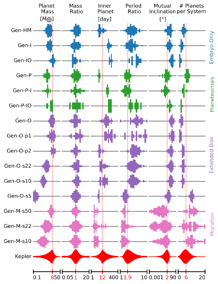
Figure 3: Distribution of planetary system properties inside 1 au averaged across all (8 or 50) runs within one set of simulations. The simulations are color-coded by accretion scenario: embryo-only (blue); planetesimals (green); extended embryo/planetesimal disk (purple); and migration (pink); The de-biased distributions derived from Kepler are shown in red, with a typical value of the distribution indicated across rows. The planet mass distribution is taken from Pascucci et al. (2018), while the distributions of planet inclination, period ratio of adjacent planets, and inner planet location are those from Mulders et al. (2018). The number of planets per system is shown as a poisson distribution with 6 planets per system. The bottom row shows the scale bar on a logarithmic stretch except for the number of planets per system which is shown on a linear scale. The peak of each distribution is normalized to span the entire y axis.

Figure 2 shows a sampling of the realizations produced within each Run Set. While variations in outcomes within a given Run Set are readily seen, it is clear that these differences are small compared to those between the different Run Sets we considered. This indicates that despite the stochastic nature of this stage of evolution, it is possible to identify signatures of the conditions under which planetary accretion took place.

Ultimately, we wish to use the relation between input parameters and realizations of planetary systems to inform the formation histories of the planetary systems found by Kepler. In order to do that, we must identify key diagnostics of the Kepler systems that can be compared to our models. Given the limited data we have on real systems, we have identified a set of broad, quantifiable parameters that describe the properties of these systems. Specifically, we use the median planet mass ($\overline{M}_{p}$), the mass ratio of adjacent planets ($\overline{\mathcal{M}}$), the median mutual inclination with respect to the invariable plane of the system, ($\overline{i}$), the median location of the innermost planet in the system, ($\overline{P}_{\text{inner}}$), the median orbital period ratio of adjacent planets, ($\overline{\mathcal{P}}$), and the median number of planets per system, $\overline{N}$. It is important to note that these parameters focus on the properties of the planetary system; that is we focus on the ensemble collection of planets, rather than the specific properties of individual planets, as these will likely inform us about how the planets interacted with one another during planet formation.

In order to ensure we are making the best comparisons between the models and the planetary systems, we focus on those planets in our simulations that are contained inside of 1 au. Because the detection efficiency of Kepler drops significantly with distance from the star, few planets are known to exist outside of that distance, making it difficult to make robust and meaningful comparisons. Note that we still allow planets to form in that region in our simulations; we just limit our statistics to those located closer to the star. Table 2 summarizes the median values and 1 $sigma$ ranges for each property for the Run Sets we considered while Figure 3 provides a visual comparison of the outcomes, providing not only the characteristic values, but also their distributions.

The parameter distributions have mostly distinct shapes between run sets, with the exception of the mass ratio distributions which are more similar across all run sets. In order to quantify the similarities between run sets we calculate the probability that the model distributions are drawn from the same underlying distribution with a KS test. Table 3 shows a set of comparions between all run sets and the base model, Gen-HM. The distributions of most parameters ($M_{p}$, $P_{\text{inner}}$, $\mathcal{P}$, $i$, and $N$) are distinguishable form the base set at high confidence ($p<0.01$). The exception is the mass ratio between adjacent planets, $\mathcal{M}$, which are statistically indistinguishable from the base set for the majority of run sets. We find the same trend when doing these comparisons between all possible combination of run sets: only the planet mass ratio distributions are often similar between models. None of the run sets are indistinguishable in all six parameter distributions, indicating that the variations in initial conditions indeed result in real differences in planetary system architectures that can be traced by these diagnostics.

Table 3: Similarities and differences between run sets. This table shows the KS-probability that the distribution of system properties (Fig. 3) are drawn from the same distribution as the base set, Gen-HM. The table headers are the same as those in Table 2. Only the mass ratio distributions are mostly consistent between the different run sets.

Run Name	${M}_{p}$ ($M_{\oplus}$)	${\mathcal{M}}$	${P}_{\text{inner}}$ (days)	${\mathcal{P}}$	${i}$ ($\deg$)	${N}$
Gen-I	0.038	0.008	$<$0.001	0.252	0.477	$<$0.001
Gen-IO	$<$0.001	0.104	$<$0.001	$<$0.001	$<$0.001	$<$0.001
Gen-P	$<$0.001	0.559	0.001	$<$0.001	$<$0.001	$<$0.001
Gen-P-I	$<$0.001	0.280	$<$0.001	$<$0.001	$<$0.001	0.997
Gen-P-IO	0.001	0.763	$<$0.001	0.183	0.307	$<$0.001
Gen-O	$<$0.001	0.067	$<$0.001	$<$0.001	$<$0.001	$<$0.001
Gen-O-p1	$<$0.001	0.028	$<$0.001	$<$0.001	$<$0.001	$<$0.001
Gen-O-p2	$<$0.001	0.022	0.481	$<$0.001	$<$0.001	0.055
Gen-O-s22	$<$0.001	0.374	$<$0.001	0.025	$<$0.001	0.272
Gen-O-s10	$<$0.001	0.132	$<$0.001	0.001	$<$0.001	$<$0.001
Gen-O-s5	$<$0.001	0.062	$<$0.001	$<$0.001	$<$0.001	$<$0.001
Gen-M-s50	$<$0.001	$<$0.001	$<$0.001	$<$0.001	$<$0.001	$<$0.001
Gen-M-s22	$<$0.001	0.005	$<$0.001	$<$0.001	$<$0.001	$<$0.001
Gen-M-s10	$<$0.001	$<$0.001	$<$0.001	$<$0.001	$<$0.001	$<$0.001

In Figure 3, we also show the approximate values and derived distributions for the Kepler exoplanets for reference. As we outline below, comparisons between the model realizations and the Kepler systems must be done with caution, and we outline a robust methodology in the next section. Before linking the properties of Kepler systems to particular formation histories, it is necessary to understand how the values of various properties are related to the initial conditions of the runs. Here we describe the effects of changes in the initial conditions on the realizations of planetary systems to provide a framework for interpreting the Kepler properties.

3.1 Effects of Including Planetesimals

Planetesimals in our models represent the leftover building blocks of planetary embryos, the more massive bodies that are the primary gravitational perturbers during the final stages of planetary accretion. Their incorporation into embryos is not expected to be 100% efficient, and as such, a number of them are expected to be present while planets form. The effects of planetesimals are seen when comparing the realizations from Run Set pairs Gen-HM & Gen-P, Gen-I & Gen-P-I, and Gen-IO & Gen-P-IO; each of these simulation pairs began with the same amount of mass present over the same radial distribution, but the latter had 25% of their mass contained in planetesimals and 75% in embryos, while the former was entirely embryos.

The primary effect of planetesimals is to provide a source of dynamical friction, where their orbits are preferentially excited to high eccentricities and inclinations while embryos and growing planets remain on more circular and roughly coplanar orbits. Inspection of Figures 2 and 3, as well as the numbers reported in Table 2 show that the inclinations of the planets formed in the embryo-only simulations are significantly higher than their planetesimal-containing pairs.

Another consequence of planetesimals being present during planetary accretion is that the number of planets that form in a given system increases. This effect is related to dynamical friction; as the embryos in the system maintain less-excited orbits, their eccentricities and inclinations are damped, limiting the semi-major axis range over which embros can collide. As a result, the feeding zones are narrower, leaving a larger number of bodies behind. This same process is also responsible for the lower masses of the planets in those cases where planetesimals were present: narrower feeding zones means fewer mass-adding events for any given planet (Figure 4a).

3.2 Effects of Inner Radius

The inner radius of our simulation defines the smallest orbital semi-major axis at which solid materials were available to form planets. In simulations for the accretion of the Solar System, this inner edge is often set at $\sim$0.5 au for computational purposes as closer-in orbits require finer time resolutions to resolve (e.g. Chambers & Wetherill, 1998; Chambers, 2004; O’Brien et al., 2006; Raymond et al., 2009). Thus, these simulations largely focus on the accretion of planets outside of this location. However, given that planetary systems discovered by Kepler contain planets located much closer to their parent stars, this requires examining the details of planet formation at these very low orbital periods.

Run Set pairs Gen-HM & Gen-I, Gen-HM & Gen-P-I, and Gen-O & Gen-IO have identical properties to one another but vary the inner edge from 0.05 au (first simulation in pair) to 0.2 au (second). In all cases, the location of the innermost planet correlates with the inner edge of the disk, with those disks extending to 0.05 au yielding innermost planets with lower periods as a result of raw materials being present closer-in for planets to form from (Figure 4b). As a result, the number of planets formed within 1 au is larger for smaller inner disk edges.

Variations in planet masses, inclinations, and period ratios are relatively minor among the Run Set pairs (Table 2). In particular, the masses of planets outside of 0.2 au are not affected by the location of the disk inner edge (Figure 4b)

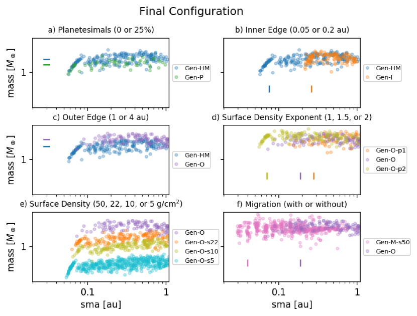
Figure 4: Simulated planet mass and semi-major axes distributions under the influence of varying one specific parameter in the initial conditions. The horizontal dashes indicate the mean mass of planets within 1 au whenever that varies significantly between simulations. The vertical dashes indicate the location of the innermost planet per system if that location varies between simulations. From left to right, top to bottom, the specific parameters/processes varied are: a) The inclusion of planetesimals, which affects planet mass (§3.1); b) The location of the disk inner edge, which affects the period of the innermost planet in each system (§3.2); c) The location of the disk outer edge, which affects the planet mass (§3.3); d) The slope of the radial surface density distribution, which affects the period of the innermost planet in each system (§3.4); e) The normalization of the surface density, which affects planet mass (§3.4); f) enabling gas-driven migration and orbital damping, which affects the period of the innermost planet in each system (§3.5).

3.3 Effects of Outer Radius

With most known extrasolar planets, particularly those in the Kepler database, found in low period orbits, many simulations for their formation have focused on the assembly of local materials inside of 1 au (Hansen & Murray, 2012, 2013; Dawson et al., 2015, 2016). However, given the decreased detection probability further from the star, it remains uncertain what the distribution of mass at larger distances may be. To investigate the effects of mass at larger distances, we performed simulations where the outer edge of the solids extended to 4 au. The outer edge of where mass may be located is likely set by a combination of the radial extent of the disk as well as how solids migrate prior to being incorporated into planetesimals.

Comparisons of Run Set pairs Gen-HM & Gen-O, Gen-P-I & Gen-P-IO, and Gen-I & Gen-IO show how the extended disk impacts the final realizations. In general, the more extended disk leads to fewer planets forming inside of 1 au, though those planets are more massive than those formed in the more truncated disks (Fig. 4c). This is likely due to the greater amount of mass in embryos and planets at larger distances, which can serve to excite the orbits of bodies close in, as well as scatter mass inward to be accreted by the planets growing in this region. The larger excitations among the growing bodies lead to a greater spacing of the planets inside of 1 au, which – in addition to reducing the number of such bodies – leads to increases in the ratio of orbital periods. Further, mutual inclinations increase as the orbits become more excited.

Thus, the amount of material in the outer disk affects the properties of planets formed inside of 1 au, consistent with the study of Ballard & Johnson (2016).

3.4 Effects of Surface Density Profile

The initial surface density profile of solids sets the total mass of embryos and planetesimals initially present in the simulation and how that mass varies with distance from the star. As described above, this is usually defined as a power-law, and thus we examined two variations of how the surface density profile of solids impacted the final realization of planets. Different surface densities may arise as disks have their masses distributed in different ways, or as radial migration of solids leads to the large-scale redistribution of solids prior to planetesimal formation.

In the first case, we considered how the surface density steepness, or exponent of the power-law, impacted the outcome of our models. These effects can be seen by comparing the realizations of Gen-O, Gen-O-p1, and Gen-O-p2 where the surface densities profiles varied as $r^{-\frac{3}{2}}$, $r^{-1}$, and $r^{-2}$, respectively. The mass ratios of adjacent planets directly correspond to the slope of the surface density distribution. A slope of $r^{-2}$ leads to roughly equal-mass planets ($\mathcal{M}=1$), while a shallow slope of $r^{-1}$ leads to the outer planets being more massive ($\mathcal{M}\approx 1.7$).

Comparing the realizations of these different runs, it is seen that more planets, with somewhat higher masses, are produced in the steeper surface density profiles, a result also seen by Raymond et al. (2005). While the total amount of mass in the simulations is greater in the shallow surface density profiles, as they extend out to 4 au, the amount interior to 1 au, where the surface density is normalized to $50$ g/cm², is greater in the steep surface profiles, thus providing more raw materials for planets to form at smaller heliocentric distances. The greater mass at larger heliocentric distances in the shallower profiles still impacts the dynamics of the interior planets, exciting them to higher inclinations and resulting in greater radial scattering of the interior planets, leaving the inner-most planet further from the star (Fig. 4d).

We also examined how the total mass of solids present in the simulations affected the properties of the final planetary system. Model Runs Gen-O, Gen-O-s22, Gen-O-s10, and Gen-O-s5 all had the same surface density steepness (varying as $r^{-\frac{3}{2}}$), but the surface density at 1 au varied, yielding different amounts of total mass to be accreted into the planets. As shown in Table 2 and Figure 4, the higher surface density runs yielded more massive planets as more material was present to be accreted. The more massive planets, due to their greater gravitational effects, cleared a larger amount of area around their orbits, leading to larger spacing between the planets, and thus fewer of them. As the total mass decreased, the amount of dynamical excitation through the system decreased, with very weak gravitational interactions taking place, leaving a large number of low mass planets behind. Similar outcomes were reported by Kokubo et al. (2006) and by Raymond et al. (2007) and Ciesla et al. (2015) in looking at the formation of planetary systems around stars of different masses: greater numbers of smaller planets were produced around stars that had lower protoplanetary disk masses. The trend of less gravitational excitement of bodies in the lower mass systems also leads to predictable results for the other quantities, with lower values for inclinations, inner planet periods, and period ratios in these same systems.

3.5 Effects of Gaseous Disk

The simulations discussed thus far have been performed assuming that the gas from the protoplanetary disk was gone by the time this stage of planetary assembly began. However, as discussed above, some of this growth may have actually occurred early in the evolution of the system while gas was still present. Such early growth is necessary in our Solar System to explain the formation of the gas giants through core accretion (e.g. Pollack et al., 1996; Hubickyj et al., 2005) and the possible early formation of Mars relative to the typical lifetime of protoplanetary disks (Dauphas & Pourmand, 2011). In addition, low bulk densities of mini-Neptunes (Wu & Lithwick, 2013; Hadden & Lithwick, 2014) and the presence of a valley in the planet radius distribution (Fulton et al., 2017; Owen & Wu, 2017) indicate that the Kepler planets likely formed in a gaseous environment.

Including disk gas in our simulations would have a dramatic effect on the dynamical evolution of planetary systems as gravitational interactions between embryos and the disk would lead to angular momentum exchange and the inward migration of the embryos. While a single migrating planet would stall at the inner edge of the gas disk, convergent migration of planets leads to inner planets in run sets migrating inside the disk inner edge, for example for run set Gen-M-s50 in Fig. 4f (see also Carrera et al. 2019).

In addition to migration, the gas also serves to damp down the eccentricities and inclinations of embryos. This is reflected in the low mutual inclinations of planets in run sets Gen-M-s50, Gen-M-s25, and Gen-M-s10 (Fig. 3.) and the large number of planets that form (as they do not get excited onto crossing orbits). As a result, the masses of individual planets tend to be much lower, but there is a greater number of planets in a given system. Further, the gas-driven migration and damping often drives planets into quasi-stable structures, thus such planets will settle into tightly-packed systems with low period ratios.

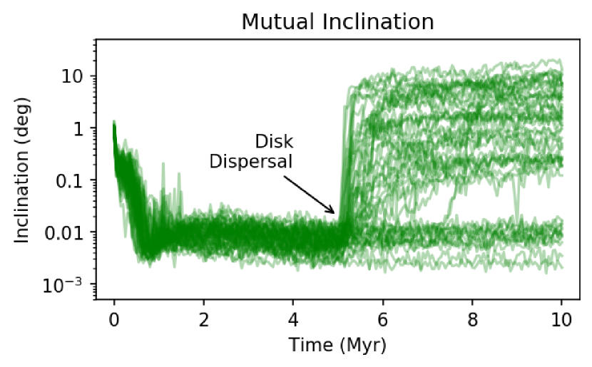
Figure 5: Time-evolution of mutual inclinations in run set Gen-M-s22, which includes gas damping and migration. The disk disperses at $5$ Myr, and system-wide instabilities occur within a few million years for a fraction of systems, after which systems remain fairly stable.

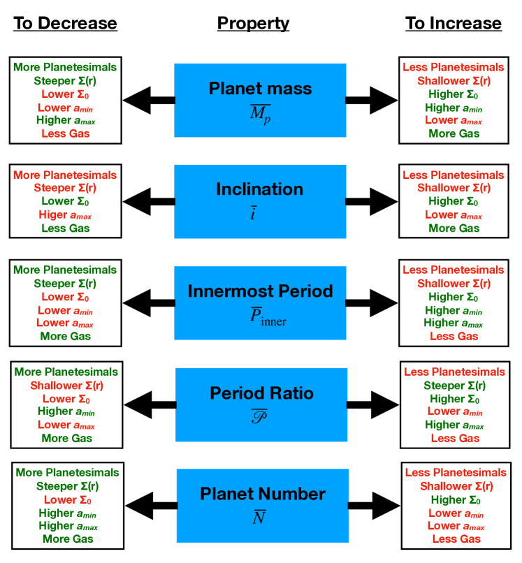
Figure 6: Summary of property dependence on N-body initial condition.

While some level of accretion may occur in the presence of gas, protoplanetary disks are estimated to retain significant gas for only 3-5 Myr before the gas is lost via photoevaporation or other processes (e.g. Ercolano & Pascucci, 2017). Here we assume the gas is present for $\sim$5 Myr, though the gas density does decrease over time (before rapidly disappearing at the end). In the absence of the gas, dynamical interactions and accretion occur as in the previously described cases. In some cases, these interactions are minimal, leaving a tightly-packed, stable system of planets. In other cases, the dynamical interactions are such that the systems go through a period of instability, leading to large increases in mutual inclination. Thus, in our simulations, as in Izidoro et al. (2017, 2019), we generally see a dichotomy in this outcome (Fig. 5), with a bimodal distribution as some systems have very low mutual inclinations while others have significantly elevated values, with few systems with mutual inclinations in between. While this is not readily apparent when looking at the median values in Table 2, it is more obvious when looking at the distributions of run sets Gen-M shown near the bottom rows of Figure 3, especially for Gen-M-s22. Although most of our simulations are relatively short ( 10 Myr), the result of the bimodal inclination distribution is likely to hold over the lifetimes of the systems: Running the simulations up to 100 Myr did not lead to a large number of these low-inclination systems becoming dynamically unstable and increasing their mutual inclinations.

It is worth noting that the presence of gas can impact the relations that develop compared to those cases where gas is not present. For example, in the higher mass surface density runs with no gas, we find that higher inclinations develop as a result of the gravitational interactions between the planets; those cases with lower surface densities have systems with lower inclinations. The opposite is true when gas is present. This is likely due to accretion occurring more rapidly when surface densities are high; given that a large amount of the gravitational interactions would take place early in the massive cases, the gas is still present to damp down any excitation that develop. As models with lower surface densities would have more protracted planet growth, the gas dissipates before planetary assembly has progressed to a similar level as in a high surface density disk, allowing the planets in the system to become more inclined. Alternatively, more massive planets experience stronger tidal damping from the gas disk.

3.6 Summary of different effects

The chaotic nature of planetary accretion means that even with similar starting conditions, the final properties of the emerging planetary systems may differ significantly from one another (Figure 2). However, given a large enough suite of simulations, it is clear that trends and relationships between the final properties and the initial conditions can be recognized (Figs. 3, 4). In this section, we have identified and explained how those trends develop for a set of final planetary system properties that can be inferred from the Kepler planetary systems.

Figure 6 summarizes how changes in individual parameters would lead to changes in the distribution of planetary systems that form. While none of our specific Run Sets exactly reproduce the properties of the Kepler systems, it is possible to use the trends and relationships that we have outlined here to adjust the parameters and components to provide a better match between the modeled and real systems. However, it is necessary to ensure that a proper comparison between the model realizations and Kepler systems is done, requiring a rigorous consideration of observational biases.

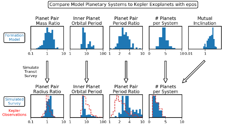
Figure 7: Comparison of simulated planetary systems with observed Kepler exoplanet systems. The top row shows the distribution of planetary system properties across run set Gen-HM. The bottom row shows a simulated Kepler survey of those systems with epos (blue), compared to the actual observations from Kepler in red. Note that planet masses from the formation model are converted to planet radii using a probabilistic mass-radius distribution before applying detection biases. Planetary system mutual inclinations are not a direct observable and are mainly constrained from the observed number of planets per system.

4 Statistical Comparison to the Kepler Planet Population

In the previous section, we discussed how various accretion scenarios lead to significantly different distributions of planetary system properties. In general, the model systems did reproduce some of the features of the Kepler populations, yielding properties that overlapped with what is observed – in particular for the model that includes planetesimals, Gen-P. However, these comparisons must be made with care, as they are done with knowledge of the full properties of the planetary systems that formed, whereas our knowledge of the observed Kepler system properties is limited by a number of observational biases. Thus, a detailed comparison between the systems produced in our models must account for these limitations in order to determine which values of the parameters for our synthetic populations would actually be detected (Fig. 7) and whether the Kepler observarions can be used to distinguish between the different accretion scenarios.

To do the forward modeling, we use epos version 3.0 (Mulders, 2020), the Exoplanet Population Observation Simulator, whose structure and detailed methodology have been described in Mulders et al. (2018, 2019). In short, epos performs a synthetic transit survey by assuming that the planetary populations produced by models make up the real distribution of planets, then performs a simulated transit survey of these systems, assuming that systems are randomly oriented along our sight lines and applies all detection biases of the Kepler spacecraft. We then compare the properties of the planets detected in the simulated survey to those of the systems detected by Kepler, which are representative of planetary systems around solar-mass stars. This approach, illustrated in Figure 7, allows for an apples-to-apples comparison between simulated planetary systems and the data, without having to parameterize the distribution of planetary system properties.

We use four observational diagnostics of planetary system properties. The first three diagnostics were defined in Mulders et al. (2019), namely the observed frequency of multi-planet systems (§4.1), the location of the innermost observed planet in each system (§4.3), and the period ratio of adjacent planets (§4.2). The fourth diagnostic is the size ratio of adjacent planets (§4.4), which has recently been shown to be strongly clustered in Kepler planetary systems (Hsu et al., 2019; Sandford et al., 2019).

An example of this observational comparison for run set Gen-HM is shown in Figure 7. The five panels in the top row show the distribution of planetary system properties from the planet formation models that are also shown in Fig. 3. The bottom panel show the four observational diagnostics calculated by epos using a forward modeling approach of the detection biases, compared to the same diagnostic calculated for the exoplanet candidates from Kepler.

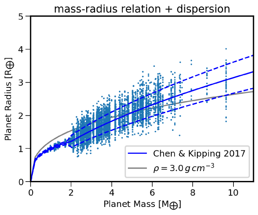
Figure 8: Mass-Radius distribution of simulated planetary systems for Gen-HM (blue-ish). The planet radii are drawn using a Monte Carlo simulation from the distribution of Chen & Kipping (2017) (dark blue), where the $1\sigma$ dispersion is indicated with the dashed lines. The constant density model assumed in the N-body integrator is shown in gray, which $\rho=3\,g/cm^{3}$.

An extra step that we perform compared to Mulders et al. (2018, 2019) is that the planet radii are calculated from the simulated masses using the planet mass-radius relation from Chen & Kipping (2017). Figure 8 shows this relation and its $1\sigma$ dispersion. For the full forward modeling in the synthetic survey, we draw the radii from a log-normal distribution centered on the best-fit mass-radius distribution using a Monte Carlo simulation. For reference, the constant density of 3 g/cm³ as used in the N-body simulation is also shown, which appears to be a reasonable value for mini-Neptunes as well.

For most runs, especially those where the inner disk edge $a_{\text{min}}$ is set to $0.05$ au, the subset that is compared to contains the majority of detected planet candidates, and thus a detailed statistical comparison can be made. In general, we find that the run sets with significantly different distributions of planetary system properties (Table 3) are also distinguishable in these observational diagnostics. This demonstrates that while some information on planetary system architectures is inevitably lost due to transit survey biases, different formation scenarios can still be constrained from the observed Kepler multi-planet systems.

For certain model runs, however, the overlap with the Kepler planet candidates is limited because few planets are formed at short orbital periods and the probability of detection of multiple planets per system is extremely low. In those cases the sub-set of observed planetary systems is too small to allow a meaningful comparison on multi-planet statistics. This is the case for runs with an inner disk edge at $a_{\text{min}}=0.2$ au (Gen-I, Gen-IO, Gen-P-I, Gen-P-IO) and the run set with a very flat surface density power-law (Gen-O-p1) that need to be compared to Kepler planet candidates outside of a $\sim 40$-day period. The data in this range contains only a handful of observed 2-planet systems, making them less likely to be relevant to the collection of planetary systems we are interested in. Thus, we omit these simulations from the following analysis.

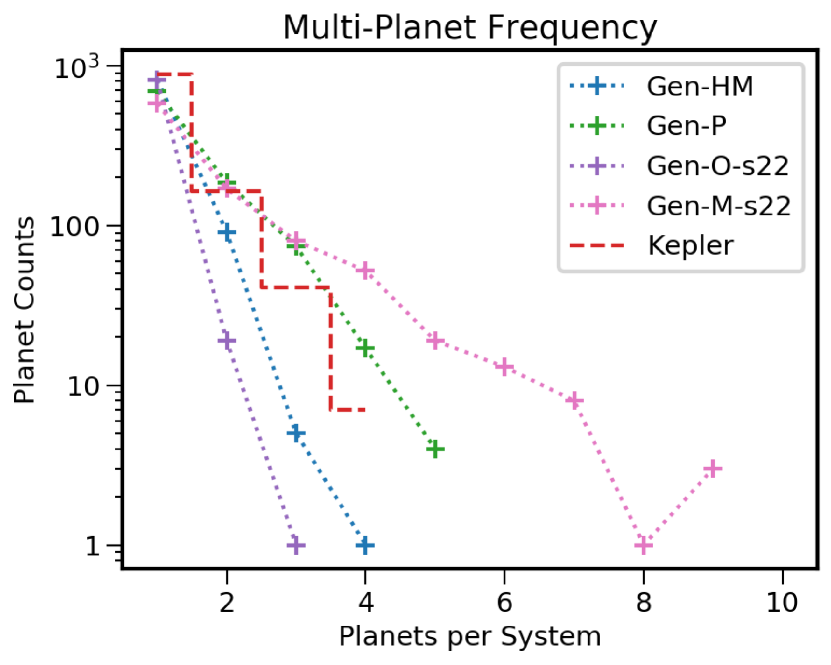
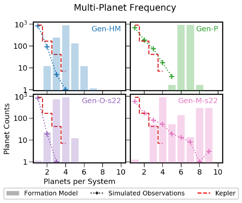
Figure 9: Observable multi-planet frequencies for different accretion scenarios. The red dashed line shows the observed frequencies from Kepler in the same range of planet radii ($1-3\,R_{\oplus}$) and orbital periods ($5-300$ days) as the simulated planets. The top panel shows the observable multi-planet frequencies for four different models to highlight the role of additional stirring when enlarging the disk outer edge (Gen-O-s22) compared to the base simulation (Gen-HM) and the role of additional damping by planetesimals (Gen-P) and gas (Gen-M-s22). The bottom panel shows how the multiplicity of planetary systems in the formation model (bars) is completely different from the observable distribution of transiting systems (plus signs) due to non-transiting planets.

4.1 Number of Planets Observed in Systems

The first diagnostic discussed here is the relative frequency of observed multi-planet systems, i.e., the observed number of stars with $m$ planets. Because most planets in multi-planet systems do not transit, this diagnostic does not always reflect the true multiplicity of systems, $N$. While most exoplanet host stars in the Kepler survey only have a single transiting planet detected, statistical studies show that most of these are members of planetary systems with multiple non-transiting planets (e.g. Lissauer et al., 2011; Zink et al., 2019). Instead, the relative frequencies are most sensitive to the mutual inclinations, with a decreased chance of observing more planets per star if the mutual inclinations are higher.

To show what the observable signature of the different planet accretion scenarios would look like, we compare four run sets that all produce planets in the same size range ($1-3\,R_{\oplus}$) and orbital period range ($5-300$ days) in Figure 9. Run Gen-HM represents an embryo-only scenario, Gen-P a planetesimal scenario, Gen-O-s22 a large disk scenario, and Gen-M-s22 a migration/damping scenario. The simulated distributions of multi-planet frequencies of these four run sets are significantly different at high confidence ($p<0.01$), showing that these diagnostics can indeed be used to discriminate between the different accretion scenarios shown in Figure 3. The observational signature of these runs are then compared to the observed frequencies of multi-planet systems from Kepler in the same ranges of planet radii and orbital periods.

The embryo-only simulations of Gen-HM under-predict the frequencies of observed 2, 3, and 4-planet systems compared to Kepler, likely because their mutual inclinations are significantly larger than the 2 degrees typically inferred for Kepler multi-planet systems (see also Fig. 3). While Hansen & Murray (2013), on which the Gen-HM runs are based, found a good match to the observed ratio of multi-planet systems, they compared their simulated planetary systems to an earlier version of the Kepler catalog that had fewer 3- and 4-planet systems. Thus, our model results are consistent with theirs, even though we find no good match to the updated Kepler systems.

Models from the Gen-O series in which the outer disk is extended to a semi-major axes of $4$ au, of which Gen-O-s22 is shown here, under-predict the number of observable 2 and 3-planet systems compared to the observations by a larger amount than Gen-HM. This is likely due to the increased dynamical stirring from the outer disk mass leading to larger mutual inclinations, which decreases the chance of multiple planets transiting from a given viewing angle (see also Moriarty & Ballard 2016). These conclusions extend to models Gen-O, Gen-O-p1, and Gen-O-s10 (not shown) which have a similar distribution of planet frequencies and are not distinguishable in this diagnostic. The multi-planet frequencies of model Gen-O-p2 are more similar to those of Gen-HM because less mass is added to the outer disk, minimizing its impact on the mutual inclinations and hence the multi-planet frequencies. The model with the lowest surface density (Gen-O-s5) has less dynamical stirring and hence lower mutual inclinations, but a direct comparison with the data is difficult because the small planet sizes yield a very small sample of detected multi-planet systems to compare to.

A better match to the observed multi-planet frequencies is seen in simulations that include planetesimals where dynamical friction reduces the mutual inclinations. Gen-P has a larger number of predicted 2–5 planet systems compared to Gen-HM, and over-predicts the observed frequencies by a small fraction. The ratio of 3/2, 4/3 and 5/4 planet systems is the same as observed, and hence this model would closely match the Kepler data if a population of single or highly inclined planets would be included to account for the Kepler dichotomy, as described in Johansen et al. (2012), Hansen & Murray (2013), and Ballard & Johnson (2016).

The inclusion of damping by gas leads to mutual inclinations that are so low that the runs over-predict the frequency of multi-planet systems. For example simulation Gen-M-s22, shown in Figure 9, which has planets in a similar size range as Gen-HM and Gen-P, over-predicts the number of 3- and 4-planet systems. Moreover, it predicts a large number of 5-8 planet systems be observed which are not present in the Kepler data in this size and period range. Simulation run sets that include migration in combination with higher and lower surface densities (Gen-M-s50 and Gen-M-s10, respectively) similarly over-predict the number of observable multi-planet systems due to their low mutual inclinations.

4.2 Period Ratios of Adjacent Planets

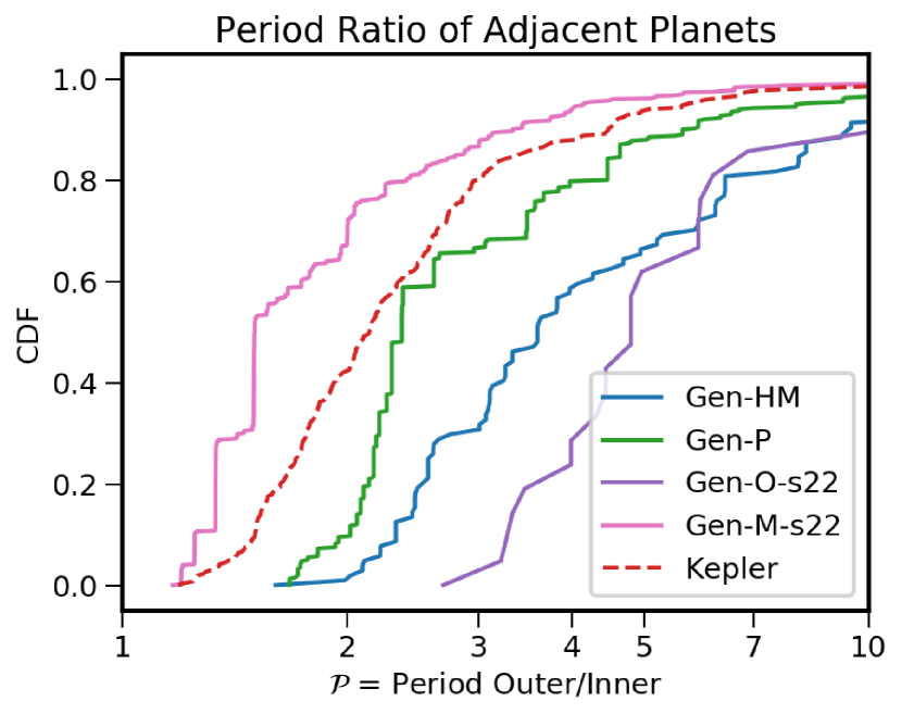
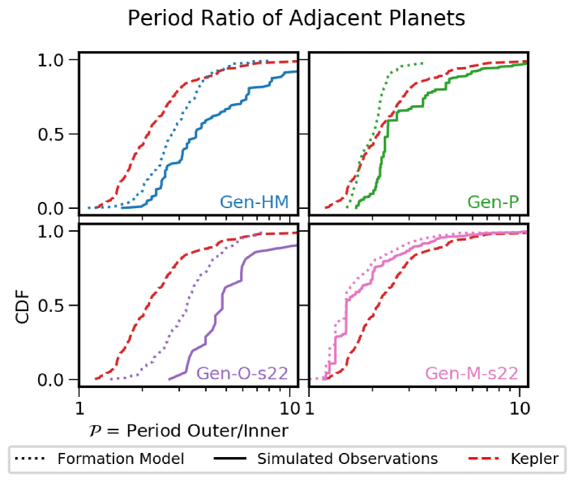
Figure 10: Period ratio distributions in a simulated survey of the different models (solid lines) compared to the Kepler observations (dashed line). These comparisons highlight the role of additional stirring when enlarging the disk outer edge (Gen-O-s22) compared to the base simulation (Gen-HM) and the role of additional damping by planetesimals (Gen-P) and gas (Gen-M-s22).

The second diagnostic discussed here is the period ratio distribution of detected planet pairs, which mainly traces the orbital spacing between planets. This period ratio is defined as $\mathcal{P}=P_{k+1}/P_{k}$ where $k$ enumerates observed planets from inside out. This diagnostic is calculated for planets in the range of $1-3R_{\oplus}$ and $5-300$ days. The detected period ratios of four models representative of different accretion scenarios are shown in Figure 10 as a cumulative distribution to highlight the excess (or absence) of resonant features. The bottom panel shows how the detected distributions are biased with respect to the distribution predicted by the formation models. The observed distribution from Kepler spans a range of period ratios from $\sim$1.3 to almost 10, with a median value at $\mathcal{P}\approx 2.2$.

The period ratio distribution of the different accretion scenarios (Fig. 10) follow a similar trend to that of the multi-planet frequencies: Simulations with the strongest damping (by gas) underpredict the observed period ratios and simulations with stronger dynamical interactions from larger disks progressively over-predict the observed period ratios.

The baseline simulation of Gen-HM (and also Gen-O-p2) has a median period ratio of $\sim 3.3$ and the distribution is located at longer period ratios compared to the observations. The amount of dynamical stirring in the embryo-only simulations leads to planets that are spaced too far apart to be consistent with the Kepler systems, as also noted by Hansen & Murray (2013). The simulations with increased mass in the outer disk (Gen-O-s22, Gen-O, Gen-O-p1) all have similar distributions with even larger period ratios due to the increased dynamical interactions. The simulations with a lower overall surface density (Gen-O-s10 and Gen-O-s5) have smaller period ratios, but because these simulations also produce smaller planets, there are not enough observed planets to allow a statistically meaningful comparison with the Kepler exoplanet population.

When dynamical friction from planetesimals are included in the simulations, the emerging planets are more tightly packed. For example the predicted period ratio distribution of simulation Gen-P has a mean period ratio of $\mathcal{P}\approx 2.4$, just higher than the observed distribution from Kepler. The shape of the distribution is roughly similar to the observed period ratio distribution, and is the closest match to the data of all the simulated systems. We did not explore if a larger number or mass fraction of planetesimals could further reduce the period ratios and provide an even better match to the observed systems.

Simulations including orbital damping by gas and planet migration, on the other hand, result in observable planetary systems that are too compact. For example, simulation Gen-M-s22 has a mean period ratio of $\mathcal{P}=1.5$ . The distributions also show strong features at the main orbital resonances (2:1 and 3:2) that are not present in the Kepler data. Dynamical instabilities that break these resonances and widen the period ratio distribution are needed to provide a better match to the observed systems, similar to recent results by Izidoro et al. (2019).

The solid surface density has a big impact on the observed period ratio distribution of planets formed in a gaseous disk. Simulations with a higher (lower) surface density of solids grow and migrate faster (slower) and therefore experience more (less) damping by gas and less (more) breaking of resonant chains. For example, simulation Gen-M-s50 with the highest solid surface density show stronger resonant features and smaller orbital periods and is therefore less consistent with the observed period ratio distribution. On the corollary, the simulation with the lowest surface density, Gen-M-s10, has fewer planets in orbital resonances and a period ratio distribution that is only slightly shortwards of the Kepler distribution. While the period ratio distributions of the three migration run sets are statistically distinguishable, they are all inconsistent with the observed distribution from Kepler.

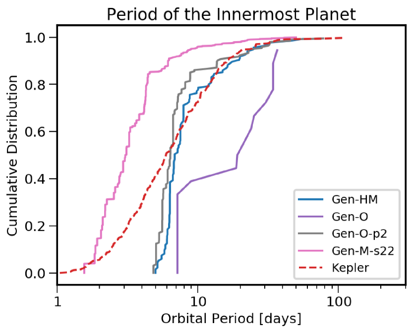
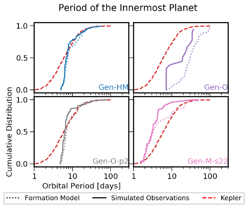
Figure 11: Period of the innermost planet in an observable multi-planet system (solid). The observed distribution from Kepler for planets in the same radius range ($1-3~{}R_{\oplus}$) is shown in dashed red. These comparisons highlight the role that migration and disk size play in determining the location of the innermost planets. All models utilize the same inner disk edge of 0.05 au. Planet migration moves the innermost planet inwards to the edge of the gas disk which is located at 0.05 au. A large outer disk results in inner planets at larger separations (Gen-O) compared to a $1$ au disk (Gen-HM) unless the outer disk contains less mass (Gen-O-p2).

4.3 Period of the Innermost Planet in Each System

The third diagnostic discussed here is the location of the innermost detected planet in an observed multi-planet system. For each system with more than one planet detected in the simulated survey, we recorded the location of the innermost detected planet. The distribution of these values is then compared to the locations of the innermost planets in the Kepler multi-planet systems. Figure 11 shows the inner planet locations for four different models in the range $1-3~{}R_{\oplus}$. Note that this is a different selection of models than in Figures 9 and 10, and was chosen to highlight the parameters that most affect the location of the inner planets.

The distributions before and after applying detection biases, shown in the bottom panel of Fig. 11, differ primarily because two detection biases are at play. First, inner planets at shorter orbital periods have an increased transit probability, which shifts the distribution of detected inner planets towards shorter periods compared to the instrinsic distribution of inner planets. Second, in a fraction of systems the inner planet is not transiting, and the innermost detected planet is located farther out, effectively broadening the distribution. epos takes both these biases into account when calculating the detectable distributions.

We find that the period of the observed innermost planet varies significantly even between simulations that have the same inner disk edge but differ in the other initial conditions (Fig. 11). The fiducial simulations of Gen-HM and Gen-P predict an observable inner period ratio distribution with roughly the same mean value as found in the Kepler data, and are not statistically distinct from each other. However, in both cases the distributions are much narrower than observed. This difference in the widths of the simulated and observed distributions could indicate that a range of inner disk locations, rather than a single value, is needed for this model to match the observed inner period distribution. Lee & Chiang (2017) have suggested that the observed spread in stellar rotation rates of young stars leads to such a range if the inner disk edge is located at the radius corresponding to the stellar co-rotation. This was also suggested by Mulders et al. (2015) based on the stellar-mass (in)dependence of the period-break in the planet occurrence rates.

Increasing the mass available by extending the outer disk (models Gen-O, Gen-O-p1) increases the amount of dynamical interactions between planets in the inner disk and also pushes the location of the innermost planets outward (see Table 2). The latter is reflected in the simulated observables, where the median inner period of model Gen-O is almost twice that of model Gen-HM (Fig. 11). The inner planet orbital period distribution is also wider than that of the fiducial model, indicating that a better fit to the data might be obtained with a larger disk but with a smaller inner disk edge. Simulation Gen-O-p2 also has an enlarged outer disk but less mass is added in this case because of the steeper surface density power-law, and this model therefore produces a comparable inner planet orbital period location distribution as run set Gen-HM.

Adding gas to the disk makes planets migrate inward, pushing the observable distribution of innermost planets inward. The median inner period of model Gen-M-s22 is more than half that of the baseline model, with a median observable period at 3 days. The simulated distribution is narrower and located at shorter orbital periods as the observed inner planet distribution. A model where the inner edge of the gas disk is located further out at an orbital period of 10 days (e.g. Mulders et al., 2018; Carrera et al., 2019), and has a dispersion in locations, would likely provide a better match to the observed Kepler systems.

4.4 Radius Ratios of Adjacent Planets

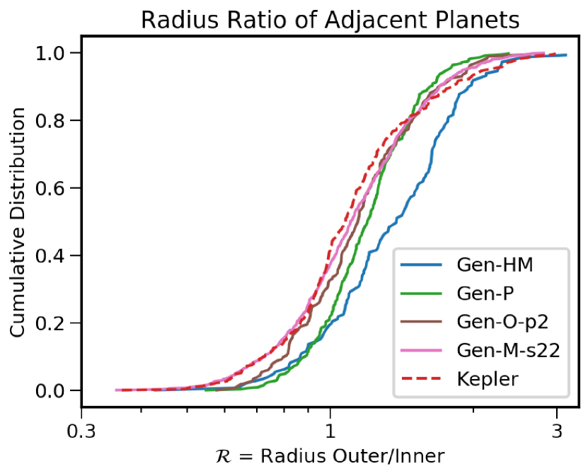
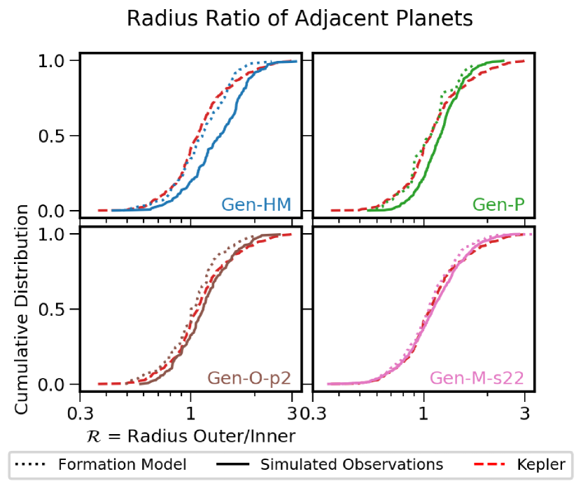
Figure 12: Radius ratio distributions in a simulated survey of the different models (solid lines) compared to the Kepler observations (dashed line).

The fourth diagnostic discussed here is the radius ratio distribution of adjacent detected planets, which mainly traces the clustering in planet sizes. This radius ratio is defined as $\mathcal{R}=R_{k+1}/R_{k}$ where $k$ enumerates observed planets from inside out. The top panel of Figure 12 shows the cumulative distribution of radius ratios for four different models in the simulated survey. Note that this is again a different selection of models than in Figures 9, 10 and 11, because the model parameters that affect the distribution of planet radii most are different. The observed distribution from Kepler for planets in the range of $1-3\,R_{\oplus}$ and $5-300$ days spans a range of radius ratios from $\sim$0.5 to almost 3. The distribution is slightly asymmetric with a median at $\mathcal{R}\approx 1.1$.

The bottom panel in (Fig. 12) shows how the size ratio distributions are affected by observation biases. The main detection bias here arises because the minimum detectable planet size increases with orbital period because fewer transits occur at large periods. A planet pair where the outer planet is larger is more likely to be detected than a planet pair where the outer planet is smaller. Thus, the size ratio distribution in the synthetic survey is shifted to larger size ratios than those in the planet formation model.

The radius ratios of the different accretion scenarios, subjected to observational biases, are shown in Figure 12. The simulated distributions typically have a similar shape as the observations in each scenario, indicating that the radius clustering of planet sizes observed with Kepler is naturally produced by these simulations. But they differ in how much they are offset toward the larger planet radius ratios. In particular, simulations Gen-HM and Gen-P are offset to larger size ratios compared to the observations.

In a scenario without migration, trends in the size ratio of planets reflect the mass distribution in the initial disk. Assuming the width of a planet’s feeding zone is proportional to its semi-major axis $a$, the surface area of the annulus that a planet accretes from scales as $a^{2}$. Models with a radial surface density exponent of $p=1.5$ are therefore expected to form planets whose mass increases with semi-major axis as $a^{0.5}$, and are thus expected to have size ratios that are on average larger than $1$. Planets formed in a disk with a radial surface density exponent of $p=2$ are expected to be of similar size at different distances from the stars. We can indeed see that simulation Gen-O-p2 does not show a significant offset compared to the observations and is a better match than simulations Gen-HM and Gen-P.

Finally, we find that simulations with migration are almost a perfect fit to the observations, showing both the same offset and dispersion in the simulated planet radius distribution as in the observations. This is perhaps slightly surprising as the underlying surface density profile used in these simulations is the same as in the gas-free simulations. Likely, the inward migration and resonant trapping changes the spacing between forming planets such that the final planetary systems end up closer to equal in mass.

5 Summary

We have explored the effects that different initial conditions and model configurations have on the final stages of planetary accretion. While the process itself is chaotic, we have identified relationships between the initial conditions and model configurations and the final planetary system properties, including the number of planets, their relative sizes, their orbital spacings, and their mutual inclinations that provide an imprint of their formation histories. Such statistical relationships can be used to inform us about the possible formation pathways of known exoplanetary systems. Doing so, however, requires a detailed assesment of the observational biases to properly reveal the properties of these systems.

In applying our knowledge to the known Kepler systems, we find that:

1. Planets within planetary systems are typically similar in size, despite the chaotic nature of the late stages of planetary assembly. In every scenario we explore, whether that includes migration of planets in a gas disk or not, the distribution of planet masses within a system are consistent with the clustering of planet radii observed with Kepler.

2. Planet formation did not occur purely through the assembly of planetary embryos as such systems would be too dynamically excited compared to the real systems. Leftover planetesimals that were present during the final stages of accretion would serve as a source of dynamical friction that provide better matches to the multi-planet frequencies and inclinations, though the simulations performed here still yield spacings between detected planets that were larger than observed.

3. Planetary systems where a significant amount of accretion occurs within a gaseous protoplanetary disk, are too dynamically cold to match the observed exoplanet population, with period ratios that are too small and have an overabundance of multi-planet systems. In contrast, systems that undergo dynamical instabilities after the disk has dispersed are dynamically hotter than those that stay stable, and the planets’ mutual inclinations within a system are closer to what is needed to match observed systems. It is, however, difficult to determine a priori which systems will go unstable and which will not.

4. The structure of the outer disk, outside of the region where planets are detected with Kepler, influences the properties of planets and planetary systems formed closer to the star, indicating that planet formation is not always a strictly local process. Planets formed in more extended disks are more massive, located farther from their host stars and are less likely to be observed as multi-planet systems.

None of the simulations performed here simultaneously matched all four observational diagnostics of planetary systems, which are the relative frequencies of multi-planet systems, the orbital period ratios of planet pairs, the size ratio of planet pairs, and the locations of the innermost planet. However, the above trends between initial conditions and observables allow us to better estimate the conditions under which these systems formed.

In regards to developing a collection of systems whose innermost planets are similar to those seen in the Kepler systems, it is necessary to consider a range of inner disk locations. The embryo-only simulations are consistent with an inner disk edge centered at 0.05 au, but future simulations should consider implementing a range for the inner disk edge rather than a single value. In more extended disks a single inner disk edge location provides a broader detected distribution that is more consistent with the data, though this inner edge has to be located closer in than 0.05 au. In simulations including migration and orbital damping by gas, the inner disk edge needs to be moved outward to $\sim 0.1$ au to result in planetary systems consistent with what is seen with Kepler.

Dynamical damping by gas in the cases studied here was too efficient, leading to too many observable multi-planets systems and planet orbital period ratios that are too low. Similar findings were found in other studies: population synthesis models with a similar number of interacting seed cores (20-50) also find mutual inclinations of planetary systems that are too low (Mulders et al., 2019); and pebble-assisted formation and migration models find that not enough systems go unstable after disk dispersal to increase their mutual inclinations to the point of reducing the number of observed planets and increasing the observed period ratios (Izidoro et al., 2017, 2019). Less efficient damping by gas may thus be necessary. For example, Dawson et al. (2016) and MacDonald et al. (2020) show that if planetary system assembly is delayed and happens when the disk gas is depleted by a factor 100 compared to the the initial gas mass, the amount of dynamical excitation matches closer to the observed systems. Although the underlying model we use has a gas density that decreases with time, we do not see this effect naturally arising from our simulations. We do see, however, that in disks that form smaller planets a closer match to the observed system properties is found. This is likely a result of these planets growing slower and, therefore, assembling when the gas density is lower or already dissipated, which, in turn, provides weaker or no orbital damping. This could suggest that the final stages of planetary accretion generally took place relatively late in terms of the removal of disk gas.

The general formation conditions outlined here allow us to make predictions about the formation pathways of habitable zone planets, and their potential chemical composition. For example, the likely presence of planetesimals during planetary accretion would provide a means for materials from more distant regions to be delivered to planets that form closer to the Sun. Such a process would be a natural means of delivering water and other volatiles to planets in the Habitable Zone.

The presence of gas might limit such radial mixing of planetesimals, but the gas would also induce type I migration, allowing planetary embryos from the outer disk to drift inwards toward the Habitable Zone. These embryos would also have formed in volatile-rich regions, allowing planets in the habitable zone to contain more water, carbon, or other bio-critical elements than if they were to have formed in situ. Since the amount of orbital damping by gas appears to be limited based on our simulation results, the influence of migration on planet composition is likely also reduced.

Quantifying the impact of different planet formation pathways on planet compositions requires an understanding of both the chemical composition in the disk as well as a model for how the distribution of material at different distances is assembled into planets. As such, we are making all simulated planetary systems discussed in this paper – complete with their accretion history – available in the Genesis database at http://eos-nexus.org/genesis-database/. The Genesis database is part of a larger effort of the Earths in Other Solar Systems (EOS) program aimed at understanding the frequency and formation of earth-like planets with bio-critical ingredients. Such a database will be instrumental in the search for extrasolar planets with atmospheric biosignatures in the Solar neighborhood.

References

- Apai et al. (2019) Apai, D., Banzatti, A., Ballering, N. P., et al. 2019, BAAS, 51, 475
- Ballard & Johnson (2016) Ballard, S., & Johnson, J. A. 2016, ApJ, 816, 66
- Batalha (2014) Batalha, N. M. 2014, Proceedings of the National Academy of Science, 111, 12647
- Bitsch et al. (2015) Bitsch, B., Johansen, A., Lambrechts, M., & Morbidelli, A. 2015, A&A, 575, A28
- Bond et al. (2010a) Bond, J. C., Lauretta, D. S., & O’Brien, D. P. 2010a, Icarus, 205, 321
- Bond et al. (2010b) Bond, J. C., O’Brien, D. P., & Lauretta, D. S. 2010b, ApJ, 715, 1050
- Burke et al. (2015) Burke, C. J., Christiansen, J. L., Mullally, F., et al. 2015, ApJ, 809, 8
- Carrera et al. (2019) Carrera, D., Ford, E. B., & Izidoro, A. 2019, MNRAS, 486, 3874
- Carter-Bond et al. (2012) Carter-Bond, J. C., O’Brien, D. P., & Raymond, S. N. 2012, ApJ, 760, 44
- Chambers (1999) Chambers, J. E. 1999, MNRAS, 304, 793
- Chambers (2001) —. 2001, Icarus, 152, 205
- Chambers (2004) —. 2004, Earth and Planetary Science Letters, 223, 241
- Chambers (2013) —. 2013, Icarus, 224, 43
- Chambers & Wetherill (1998) Chambers, J. E., & Wetherill, G. W. 1998, Icarus, 136, 304
- Chen & Kipping (2017) Chen, J., & Kipping, D. 2017, ApJ, 834, 17
- Christiansen et al. (2016) Christiansen, J. L., Clarke, B. D., Burke, C. J., et al. 2016, ApJ, 828, 99
- Ciesla et al. (2015) Ciesla, F. J., Mulders, G. D., Pascucci, I., & Apai, D. 2015, ApJ, 804, 9
- Coleman & Nelson (2014) Coleman, G. A. L., & Nelson, R. P. 2014, MNRAS, 445, 479
- Cresswell & Nelson (2006) Cresswell, P., & Nelson, R. P. 2006, A&A, 450, 833
- Cresswell & Nelson (2008) —. 2008, A&A, 482, 677
- Dauphas & Pourmand (2011) Dauphas, N., & Pourmand, A. 2011, Nature, 473, 489
- Dawson et al. (2015) Dawson, R. I., Chiang, E., & Lee, E. J. 2015, MNRAS, 453, 1471
- Dawson et al. (2016) Dawson, R. I., Lee, E. J., & Chiang, E. 2016, ApJ, 822, 54
- Duncan et al. (1998) Duncan, M. J., Levison, H. F., & Lee, M. H. 1998, AJ, 116, 2067
- Ercolano & Pascucci (2017) Ercolano, B., & Pascucci, I. 2017, Royal Society Open Science, 4, 170114
- Fendyke & Nelson (2014) Fendyke, S. M., & Nelson, R. P. 2014, MNRAS, 437, 96
- Fischer & Ciesla (2014) Fischer, R. A., & Ciesla, F. J. 2014, Earth and Planetary Science Letters, 392, 28
- Fulton et al. (2017) Fulton, B. J., Petigura, E. A., Howard, A. W., et al. 2017, AJ, 154, 109
- Hadden & Lithwick (2014) Hadden, S., & Lithwick, Y. 2014, ApJ, 787, 80
- Hansen & Murray (2012) Hansen, B. M. S., & Murray, N. 2012, ApJ, 751, 158
- Hansen & Murray (2013) —. 2013, ApJ, 775, 53
- Hsu et al. (2019) Hsu, D. C., Ford, E. B., Ragozzine, D., & Ashby, K. 2019, The Astronomical Journal, 158, 109
- Hubickyj et al. (2005) Hubickyj, O., Bodenheimer, P., & Lissauer, J. J. 2005, Icarus, 179, 415
- Hunter (2007) Hunter, J. D. 2007, Computing in Science & Engineering, 9, 90
- Izidoro et al. (2019) Izidoro, A., Bitsch, B., Raymond, S. N., et al. 2019, arXiv e-prints, arXiv:1902.08772
- Izidoro et al. (2013) Izidoro, A., de Souza Torres, K., Winter, O. C., & Haghighipour, N. 2013, ApJ, 767, 54
- Izidoro et al. (2014) Izidoro, A., Haghighipour, N., Winter, O. C., & Tsuchida, M. 2014, ApJ, 782, 31
- Izidoro et al. (2017) Izidoro, A., Ogihara, M., Raymond, S. N., et al. 2017, MNRAS, 470, 1750
- Johansen et al. (2012) Johansen, A., Davies, M. B., Church, R. P., & Holmelin, V. 2012, ApJ, 758, 39
- Jones et al. (2001–) Jones, E., Oliphant, T., Peterson, P., et al. 2001–, SciPy: Open source scientific tools for Python, [Online; accessed <today>]
- Kokubo & Ida (2000) Kokubo, E., & Ida, S. 2000, Icarus, 143, 15
- Kokubo et al. (2006) Kokubo, E., Kominami, J., & Ida, S. 2006, The Astrophysical Journal, 642, 1131
- Lee & Chiang (2017) Lee, E. J., & Chiang, E. 2017, ApJ, 842, 40
- Lissauer (2007) Lissauer, J. J. 2007, ApJ, 660, L149
- Lissauer et al. (2011) Lissauer, J. J., Ragozzine, D., Fabrycky, D. C., et al. 2011, ApJS, 197, 8
- MacDonald et al. (2020) MacDonald, M. G., Dawson, R. I., Morrison, S. J., Lee, E. J., & Khandelwal, A. 2020, ApJ, 891, 20
- Moriarty & Ballard (2016) Moriarty, J., & Ballard, S. 2016, ApJ, 832, 34
- Mulders (2020) Mulders, G. D. 2020, EPOS: The Exoplanet Population Observation Simulator, https://doi.org/10.5281/zenodo.3764219
- Mulders et al. (2019) Mulders, G. D., Mordasini, C., Pascucci, I., et al. 2019, arXiv e-prints, arXiv:1905.08804 [astro-ph.EP]
- Mulders et al. (2015) Mulders, G. D., Pascucci, I., & Apai, D. 2015, The Astrophysical Journal, 798, 112
- Mulders et al. (2018) Mulders, G. D., Pascucci, I., Apai, D., & Ciesla, F. J. 2018, ArXiv e-prints, arXiv:1805.08211 [astro-ph.EP]
- O’Brien et al. (2006) O’Brien, D. P., Morbidelli, A., & Levison, H. F. 2006, Icarus, 184, 39
- O’Brien et al. (2014) O’Brien, D. P., Walsh, K. J., Morbidelli, A., Raymond, S. N., & Mandell, A. M. 2014, Icarus, 239, 74
- Ogihara et al. (2015) Ogihara, M., Morbidelli, A., & Guillot, T. 2015, A&A, 584, L1
- Owen & Wu (2017) Owen, J. E., & Wu, Y. 2017, ApJ, 847, 29
- Paardekooper et al. (2010) Paardekooper, S.-J., Baruteau, C., Crida, A., & Kley, W. 2010, MNRAS, 401, 1950
- Paardekooper et al. (2011) Paardekooper, S.-J., Baruteau, C., & Kley, W. 2011, MNRAS, 410, 293
- Papaloizou & Larwood (2000) Papaloizou, J. C. B., & Larwood, J. D. 2000, MNRAS, 315, 823
- Pascucci et al. (2018) Pascucci, I., Mulders, G. D., Gould, A., & Fernandes, R. 2018, The Astrophysical Journal Letters, 856, L28
- Pollack et al. (1996) Pollack, J. B., Hubickyj, O., Bodenheimer, P., et al. 1996, Icarus, 124, 62
- Quintana et al. (2007) Quintana, E. V., Adams, F. C., Lissauer, J. J., & Chambers, J. E. 2007, ApJ, 660, 807
- Quintana & Lissauer (2014) Quintana, E. V., & Lissauer, J. J. 2014, ApJ, 786, 33
- Raymond et al. (2014) Raymond, S. N., Kokubo, E., Morbidelli, A., Morishima, R., & Walsh, K. J. 2014, in Protostars and Planets VI, ed. H. Beuther, R. S. Klessen, C. P. Dullemond, & T. Henning, 595
- Raymond et al. (2009) Raymond, S. N., O’Brien, D. P., Morbidelli, A., & Kaib, N. A. 2009, Icarus, 203, 644
- Raymond et al. (2004) Raymond, S. N., Quinn, T., & Lunine, J. I. 2004, Icarus, 168, 1
- Raymond et al. (2005) —. 2005, ApJ, 632, 670
- Raymond et al. (2006) —. 2006, Icarus, 183, 265
- Raymond et al. (2007) Raymond, S. N., Scalo, J., & Meadows, V. S. 2007, ApJ, 669, 606
- Sandford et al. (2019) Sandford, E., Kipping, D., & Collins, M. 2019, Monthly Notices of the Royal Astronomical Society, 489, 3162
- Tanaka & Ward (2004) Tanaka, H., & Ward, W. R. 2004, ApJ, 602, 388
- Thompson et al. (2017) Thompson, S. E., Coughlin, J. L., Hoffman, K., et al. 2017, ArXiv e-prints, arXiv:1710.06758 [astro-ph.EP]
- van der Walt et al. (2011) van der Walt, S., Colbert, S. C., & Varoquaux, G. 2011, Computing in Science & Engineering, 13, 22
- Walsh et al. (2011) Walsh, K. J., Morbidelli, A., Raymond, S. N., O’Brien, D. P., & Mandell, A. M. 2011, Nature, 475, 206
- Wetherill (1994) Wetherill, G. W. 1994, Geochim. Cosmochim. Acta, 58, 4513
- Wetherill & Stewart (1993) Wetherill, G. W., & Stewart, G. R. 1993, Icarus, 106, 190
- Wu & Lithwick (2013) Wu, Y., & Lithwick, Y. 2013, ApJ, 772, 74
- Zink et al. (2019) Zink, J. K., Christiansen, J. L., & Hansen, B. M. S. 2019, MNRAS, 483, 4479