Text-Based Ideal Points

Abstract

Ideal point models analyze lawmakers’ votes to quantify their political positions, or ideal points. But votes are not the only way to express a political position. Lawmakers also give speeches, release press statements, and post tweets. In this paper, we introduce the text-based ideal point model (tbip), an unsupervised probabilistic topic model that analyzes texts to quantify the political positions of its authors. We demonstrate the tbip with two types of politicized text data: U.S. Senate speeches and senator tweets. Though the model does not analyze their votes or political affiliations, the tbip separates lawmakers by party, learns interpretable politicized topics, and infers ideal points close to the classical vote-based ideal points. One benefit of analyzing texts, as opposed to votes, is that the tbip can estimate ideal points of anyone who authors political texts, including non-voting actors. To this end, we use it to study tweets from the 2020 Democratic presidential candidates. Using only the texts of their tweets, it identifies them along an interpretable progressive-to-moderate spectrum.

1 Introduction

Figure 1: The tbip separates senators by political party using only speeches. The algorithm does not have access to party information, but senators are coded by their political party for clarity (Democrats in blue circles, Republicans in red x’s). The speeches are from the 114th U.S. Senate.

Ideal point models are widely used to help characterize modern democracies, analyzing lawmakers’ votes to estimate their positions on a political spectrum (Poole and Rosenthal, 1985). But votes aren’t the only way that lawmakers express political preferences—press releases, tweets, and speeches all help convey their positions. Like votes, these signals are recorded and easily collected.

This paper develops the text-based ideal point model (tbip), a probabilistic topic model for analyzing unstructured political texts to quantify the political preferences of their authors. While classical ideal point models analyze how different people vote on a shared set of bills, the tbip analyzes how different authors write about a shared set of latent topics. The tbip is inspired by the idea of political framing: the specific words and phrases used when discussing a topic can convey political messages (Entman, 1993). Given a corpus of political texts, the tbip estimates the latent topics under discussion, the latent political positions of the authors of texts, and how per-topic word choice changes as a function of the political position of the author.

A key feature of the tbip is that it is unsupervised. It can be applied to any political text, regardless of whether the authors belong to known political parties. It can also be used to analyze non-voting actors, such as political candidates.

Figure 1 shows a tbip analysis of the speeches of the 114th U.S. Senate. The model lays the senators out on the real line and accurately separates them by party. (It does not use party labels in its analysis.) Based only on speeches, it has found an interpretable spectrum—Senator Bernie Sanders is liberal, Senator Mitch McConnell is conservative, and Senator Susan Collins is moderate. For comparison, Figure 2 also shows ideal points estimated from the voting record of the same senators; their language and their votes are closely correlated.

The tbip also finds latent topics, each one a vocabulary-length vector of intensities, that describe the issues discussed in the speeches. For each topic, the tbip involves both a neutral vector of intensities and a vector of ideological adjustments that describe how the intensities change as a function of the political position of the author. Illustrated in Table 1 are discovered topics about immigration, health care, and gun control. In the gun control topic, the neutral intensities focus on words like “gun” and “firearms.” As the author’s ideal point becomes more negative, terms like “gun violence” and “background checks” increase in intensity. As the author’s ideal point becomes more positive, terms like “constitutional rights” increase.

The tbip is a bag-of-words model that combines ideas from ideal point models and Poisson factorization topic models (Canny, 2004; Gopalan et al., 2015). The latent variables are the ideal points of the authors, the topics discussed in the corpus, and how those topics change as a function of ideal point. To approximate the posterior, we use an efficient black box variational inference algorithm with stochastic optimization. It scales to large corpora.

We develop the details of the tbip and its variational inference algorithm. We study its performance on three sessions of U.S. Senate speeches, and we compare the tbip to other methods for scaling political texts (Slapin and Proksch, 2008; Lauderdale and Herzog, 2016a). The tbip performs best, recovering ideal points closest to the vote-based ideal points. We also study its performance on tweets by U.S. senators, again finding that it closely recovers their vote-based ideal points. (In both speeches and tweets, the differences from vote-based ideal points are also qualitatively interesting.) Finally, we study the tbip on tweets by the 2020 Democratic candidates for President, for which there are no votes for comparison. It lays out the candidates along an interpretable progressive-to-moderate spectrum.

2 The text-based ideal point model

We develop the text-based ideal point model (tbip), a probabilistic model that infers political ideology from political texts. We first review Bayesian ideal points and Poisson factorization topic models, two probabilistic models on which the tbip is built.

2.1 Background: Bayesian ideal points

Ideal points quantify a lawmaker’s political preferences based on their roll-call votes (Poole and Rosenthal, 1985; Jackman, 2001; Clinton et al., 2004). Consider a group of lawmakers voting “yea” or “nay” on a shared set of bills. Denote the vote of lawmaker $i$ on bill $j$ by the binary variable $v_{ij}$. The Bayesian ideal point model posits scalar per-lawmaker latent variables $x_{i}$ and scalar per-bill latent variables $(\alpha_{j},\eta_{j})$. It assumes the votes come from a factor model,

$$x_{i} \sim\mathcal{N}(0,1)$$

$$\alpha_{j},\eta_{j} \sim\mathcal{N}(0,1)$$

$$v_{ij} \sim\text{Bern}(\sigma(\alpha_{j}+x_{i}\eta_{j})).$$ (1)

where $\sigma(t)=\frac{1}{1+e^{-t}}$.

The latent variable $x_{i}$ is called the lawmaker’s ideal point; the latent variable $\eta_{j}$ is the bill’s polarity. When $x_{i}$ and $\eta_{j}$ have the same sign, lawmaker $i$ is more likely to vote for bill $j$; when they have opposite sign, the lawmaker is more likely to vote against it. The per-bill intercept term $\alpha_{j}$ is called the popularity. It captures that some bills are uncontroversial, where all lawmakers are likely to vote for them (or against them) regardless of their ideology.

Using data of lawmakers voting on bills, political scientists approximate the posterior of the Bayesian ideal point model with an approximate inference method such as Markov Chain Monte Carlo (MCMC) (Jackman, 2001; Clinton et al., 2004) or expectation-maximization (EM) (Imai et al., 2016). Empirically, the posterior ideal points of the lawmakers accurately separate political parties and capture the spectrum of political preferences in American politics (Poole and Rosenthal, 2000).

2.2 Background: Poisson factorization

Poisson factorization is a class of non-negative matrix factorization methods often employed as a topic model for bag-of-words text data (Canny, 2004; Cemgil, 2009; Gopalan et al., 2014).

Poisson factorization factorizes a matrix of document/word counts into two positive matrices: a matrix $\boldsymbol{\theta}$ that contains per-document topic intensities, and a matrix $\boldsymbol{\beta}$ that contains the topics. Denote the count of word $v$ in document $d$ by $y_{dv}$. Poisson factorization posits the following probabilistic model over word counts, where $a$ and $b$ are hyperparameters:

$$\theta_{dk} \sim\textrm{Gamma}(a,b)$$

$$\beta_{kv} \sim\textrm{Gamma}(a,b)$$

$$y_{dv} \sim\text{Pois}\left(\textstyle\sum_{k}\theta_{dk}\beta_{kv}\right).$$ (2)

Given a matrix $\boldsymbol{y}$, practitioners approximate the posterior factorization with variational inference (Gopalan et al., 2015) or MCMC (Cemgil, 2009). Note that Poisson factorization can be interpreted as a Bayesian variant of nonnegative matrix factorization, with the so-called “KL loss function” (Lee and Seung, 1999).

When the shape parameter $a$ is less than 1, the latent vectors $\theta_{d}$ and $\beta_{k}$ tend to be sparse. Consequently, the marginal likelihood of each count places a high mass around zero and has heavy tails (Ranganath et al., 2015). The posterior components are interpretable as topics (Gopalan et al., 2015).

Ideology Top Words Liberal dreamers, dream, undocumented, daca, comprehensive immigration reform, deport, young, deportation Neutral immigration, united states, homeland security, department, executive, presidents, law, country Conservative laws, homeland security, law, department, amnesty, referred, enforce, injunction Liberal affordable care act, seniors, medicare, medicaid, sick, prescription drugs, health insurance, million americans Neutral health care, obamacare, affordable care act, health insurance, insurance, americans, coverage, percent Conservative health care law, obamacare, obama, democrats, obamacares, deductibles, broken promises, presidents health care Liberal gun violence, gun, guns, killed, hands, loophole, background checks, close Neutral gun, guns, second, orlando, question, firearms, shooting, background checks Conservative second, constitutional rights, rights, due process, gun control, mental health, list, mental illness

Table 1: The tbip learns topics from Senate speeches that vary as a function of the senator’s political positions. The neutral topics are for an ideal point of 0; the ideological topics fix ideal points at $-1$ and $+1$. We interpret one extreme as liberal and the other as conservative. Data is from the 114th U.S. Senate.

2.3 The text-based ideal point model

The text-based ideal point model (tbip) is a probabilistic model that is designed to infer political preferences from political texts.

There are important differences between a dataset of votes and a corpus of authored political language. A vote is one of two choices, “yea” or “nay.” But political language is high dimensional—a lawmaker’s speech involves a vocabulary of thousands. A vote sends a clear signal about a lawmaker’s opinion about a bill. But political speech is noisy—the use of a word might be irrelevant to ideology, provide only a weak signal about ideology, or change signal depending on context. Finally, votes are organized in a matrix, where each one is unambiguously attached to a specific bill and nearly all lawmakers vote on all bills. But political language is unstructured and sparse. A corpus of political language can discuss any number of issues—with speeches possibly involving several issues—and the issues are unlabeled and possibly unknown in advance.

The tbip is based on the concept of political framing. Framing is the idea that a communicator will emphasize certain aspects of a message – implicitly or explicitly – to promote a perspective or agenda (Entman, 1993; Chong and Druckman, 2007). In politics, an author’s word choice for a particular issue is affected by the ideological message she is trying to convey. A conservative discussing abortion is more likely to use terms such as “life” and “unborn,” while a liberal discussing abortion is more likely to use terms like “choice” and “body.” In this example, a conservative is framing the issue in terms of morality, while a liberal is framing the issue in terms of personal liberty.

The tbip casts political framing in a probabilistic model of language. While the classical ideal point model infers ideology from the differences in votes on a shared set of bills, the tbip infers ideology from the differences in word choice on a shared set of topics.

The tbip is a probabilistic model that builds on Poisson factorization. The observed data are word counts and authors: $y_{dv}$ is the word count for term $v$ in document $d$, and $a_{d}$ is the author of the document. Some of the latent variables in the tbip are inherited from Poisson factorization: the non-negative $K$-vector of per-document topic intensities is $\theta_{d}$ and the topics themselves are non-negative $V$-vectors $\beta_{k}$, where $K$ is the number of topics and $V$ is the vocabulary size. We refer to $\boldsymbol{\beta}$ as the neutral topics. Two additional latent variables capture the politics: the ideal point of an author $s$ is a real-valued scalar $x_{s}$, and the ideological topic is a real-valued $V$-vector $\eta_{k}$.

The tbip uses its latent variables in a generative model of authored political text, where the ideological topic adjusts the neutral topic—and thus the word choice—as a function of the ideal point of the author. Place sparse Gamma priors on $\boldsymbol{\theta}$ and $\boldsymbol{\beta}$, and normal priors on $\boldsymbol{\eta}$ and $\boldsymbol{x}$, so for all documents $d$, words $v$, topics $k$, and authors $s$,

$$\theta_{dk} \sim\textrm{Gamma}(a,b) \eta_{kv} \sim\mathcal{N}(0,1)$$

$$\beta_{kv} \sim\textrm{Gamma}(a,b) x_{s} \sim\mathcal{N}(0,1).$$

These latent variables interact to draw the count of term $v$ in document $d$,

$$y_{dv} \sim\textstyle\textrm{Pois}\left(\sum_{k}\theta_{dk}\beta_{kv}\exp\{x_{a_{d}}\eta_{kv}\}\right).$$ (3)

For a topic $k$ and term $v$, a non-zero $\eta_{kv}$ will increase the Poisson rate of the word count if it shares the same sign as the ideal point of the author $x_{a_{d}}$, and decrease the Poisson rate if they are of opposite signs. Consider a topic about gun control and suppose $\eta_{kv}>0$ for the term “constitution.” An author with an ideal point $x_{s}>0$, say a conservative author, will be more likely to use the term “constitution” when discussing gun control; an author with an ideal point $x_{s}<0$, a liberal author, will be less likely to use the term. Suppose $\eta_{kv}<0$ for the term “violence.” Now the liberal author will be more likely than the conservative to use this term. Finally suppose $\eta_{kv}=0$ for the term “gun.” This term will be equally likely to be used by the authors, regardless of their ideal points.

To build more intuition, examine the elements of the sum in the Poisson rate of Equation 3 and rewrite slightly to $\theta_{dk}\exp(\log\beta_{kv}+x_{a_{d}}\eta_{kv})$. Each of these elements mimics the classical ideal point model in Section 2.1, where $\eta_{kv}$ now measures the “polarity” of term $v$ in topic $k$ and $\log\beta_{kv}$ is the intercept or “popularity.” When $\eta_{kv}$ and $x_{a_{d}}$ have the same sign, term $v$ is more likely to be used when discussing topic $k$. If $\eta_{kv}$ is near zero, then the term is not politicized, and its count comes from a Poisson factorization. For each document $d$, the elements of the sum that contribute to the overall rate are those for which $\theta_{dk}$ is positive; that is, those for the topics that are being discussed in the document.

The posterior distribution of the latent variables provides estimates of the ideal points, neutral topics, and ideological topics. For example, we estimate this posterior distribution using a dataset of senator speeches from the 114th United States Senate session. The fitted ideal points in Figure 1 show that the tbip largely separates lawmakers by political party, despite not having access to these labels or votes. Table 1 depicts neutral topics (fixing the fitted $\hat{\eta}_{kv}$ to be 0) and the corresponding ideological topics by varying the sign of $\hat{\eta}_{kv}$. The topic for immigration shows that a liberal framing emphasizes “Dreamers” and “DACA”, while the conservative frame emphasizes “laws” and “homeland security.” We provide more details and empirical studies in Section 5.

3 Related work

Most ideal point models focus on legislative roll-call votes. These are typically latent-space factor models (Poole and Rosenthal, 1985; McCarty et al., 1997; Poole and Rosenthal, 2000), which relate closely to item-response models (Bock and Aitkin, 1981; Bailey, 2001). Researchers have also developed Bayesian analogues (Jackman, 2001; Clinton et al., 2004) and extensions to time series, particularly for analyzing the Supreme Court (Martin and Quinn, 2002).

Some recent models combine text with votes or party information to estimate ideal points of legislators. Gerrish and Blei (2011) analyze votes and the text of bills to learn ideological language. Gerrish and Blei (2012), Lauderdale and Clark (2014), and Song et al. (2018) use text and vote data to learn ideal points adjusted for topic. The models in Nguyen et al. (2015) and Kim et al. (2018) analyze votes and floor speeches together. With labeled political party affiliations, machine learning methods can also help map language to party membership. Iyyer et al. (2014) use neural networks to learn partisan phrases, while the models in Tsur et al. (2015) and Gentzkow et al. (2019) use political party labels to analyze differences in speech patterns. Since the tbip does not use votes or party information, it is applicable to all political texts, even when votes and party labels are not present. Moreover, party labels can be restrictive because they force hard membership in one of two groups (in American politics). The tbip can infer how topics change smoothly across the political spectrum, rather than simply learning topics for each political party.

Annotated text data has also been used to predict ideological positions. Wordscores (Laver et al., 2003; Lowe, 2008) uses texts that are hand-labeled by political position to measure the conveyed positions of unlabeled texts; it has been used to measure the political landscape of Ireland (Benoit and Laver, 2003; Herzog and Benoit, 2015). Ho et al. (2008) analyze hand-labeled editorials to estimate ideal points for newspapers. The ideological topics learned by the tbip are also related to political frames (Entman, 1993; Chong and Druckman, 2007). Historically, these frames have either been hand-labeled by annotators (Baumgartner et al., 2008; Card et al., 2015) or used annotated data for supervised prediction (Johnson et al., 2017; Baumer et al., 2015). In contrast to these methods, the tbip is completely unsupervised. It learns ideological topics that do not need to conform to pre-defined frames. Moreover, it does not depend on the subjectivity of coders.

wordfish (Slapin and Proksch, 2008) is a model of authored political texts about a single issue, similar to a single-topic version of tbip. wordfish has been applied to party manifestos (Proksch and Slapin, 2009; Lo et al., 2016) and single-issue dialogue (Schwarz et al., 2017). wordshoal (Lauderdale and Herzog, 2016a) extends wordfish to multiple issues by analyzing a collection of labeled texts, such as Senate speeches labeled by debate topic. wordshoal fits separate wordfish models to the texts about each label, and combines the fitted models in a one-dimensional factor analysis to produce ideal points. In contrast to these models, the tbip does not require a grouping of the texts into single issues. It naturally accommodates unstructured texts, such as tweets, and learns both ideal points for the authors and ideology-adjusted topics for the (latent) issues under discussion. Furthermore, by relying on stochastic optimization, the tbip algorithm scales to large data sets. In Section 5 we empirically study how the tbip ideal points compare to both of these models.

4 Inference

The tbip involves several types of latent variables: neutral topics $\beta_{k}$, ideological topics $\eta_{k}$, topic intensities $\theta_{d}$, and ideal points $x_{s}$. Conditional on the text, we perform inference of the latent variables through the posterior distribution $p(\boldsymbol{\theta},\boldsymbol{\beta},\boldsymbol{\eta},\boldsymbol{x}|\boldsymbol{y})$. But calculating this distribution is intractable. We rely on approximate inference.

We use mean-field variational inference to fit an approximate posterior distribution (Jordan et al., 1999; Wainwright et al., 2008; Blei et al., 2017). Variational inference frames the inference problem as an optimization problem. Set $q_{\phi}(\boldsymbol{\theta},\boldsymbol{\beta},\boldsymbol{\eta},\boldsymbol{x})$ to be a variational family of approximate posterior distributions, indexed by variational parameters $\phi$. Variational inference aims to find the setting of $\phi$ that minimizes the KL divergence between $q_{\phi}$ and the posterior.

Minimizing this KL divergence is equivalent to maximizing the evidence lower bound (elbo),

$$\mathbb{E}_{q_{\phi}}[\log p(\boldsymbol{\theta},\boldsymbol{\beta},\boldsymbol{\eta},\boldsymbol{x}) +\log p(\boldsymbol{y}|\boldsymbol{\theta},\boldsymbol{\beta},\boldsymbol{\eta},\boldsymbol{x})$$

$$-\log q_{\phi}(\boldsymbol{\theta},\boldsymbol{\beta},\boldsymbol{\eta},\boldsymbol{x})].$$

The elbo sums the expectation of the log joint—here broken up into the log prior and log likelihood—and the entropy of the variational distribution.

To approximate the tbip posterior we set the variational family to be the mean-field family. The mean-field family factorizes over the latent variables, where $d$ indexes documents, $k$ indexes topics, and $s$ indexes authors:

$$q_{\phi}(\boldsymbol{\theta},\boldsymbol{\beta},\boldsymbol{\eta},\boldsymbol{x})=\prod_{d,k,s}q(\theta_{d})q(\beta_{k})q(\eta_{k})q(x_{s}).$$

We use lognormal factors for the positive variables and Gaussian factors for the real variables,

$$q(\theta_{d}) =\mathrm{LogNormal}_{K}(\mu_{\theta_{d}},I\sigma^{2}_{\theta_{d}})$$

$$q(\beta_{k}) =\mathrm{LogNormal}_{V}(\mu_{\beta_{k}},I\sigma^{2}_{\beta_{k}})$$

$$q(\eta_{k}) =\mathcal{N}_{V}(\mu_{\eta_{k}},I\sigma^{2}_{\eta_{k}})$$

$$q(x_{s}) =\mathcal{N}(\mu_{x_{s}},\sigma^{2}_{x_{s}}).$$

Our goal is to optimize the elbo with respect to $\phi=\{\boldsymbol{\mu}_{\theta},\boldsymbol{\sigma}^{2}_{\theta},\boldsymbol{\mu}_{\beta},\boldsymbol{\sigma}^{2}_{\beta},\boldsymbol{\mu}_{\eta},\boldsymbol{\sigma}^{2}_{\eta},\boldsymbol{\mu}_{x},\boldsymbol{\sigma}^{2}_{x}\}$.

We use stochastic gradient ascent. We form noisy gradients with Monte Carlo and the “reparameterization trick” (Kingma and Welling, 2014; Rezende et al., 2014), as well as with data subsampling (Hoffman et al., 2013). To set the step size, we use Adam (Kingma and Ba, 2015).

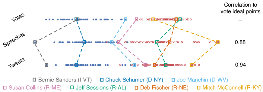
Figure 2: The ideal points learned by the tbip for senator speeches and tweets are highly correlated with the classical vote ideal points. Senators are coded by their political party (Democrats in blue circles, Republicans in red x’s). Although the algorithm does not have access to these labels, the tbip almost completely separates parties.

We initialize the neutral topics and topic intensities with a pre-trained model. Specifically, we pre-train a Poisson factorization topic model using the algorithm in Gopalan et al. (2015). The tbip algorithm uses the resulting factorization to initialize the variational parameters for $\theta_{d}$ and $\beta_{k}$. The full procedure is described in Appendix A.

For the corpus of Senate speeches described in Section 2, training takes 5 hours on a single NVIDIA Titan V GPU. We have released open source software in Tensorflow and PyTorch.

5 Empirical studies

We study the text-based ideal point model (tbip) on several datasets of political texts. We first use the tbip to analyze speeches and tweets (separately) from U.S. senators. For both types of texts, the tbip ideal points, which are estimated from text, are close to the classical ideal points, which are estimated from votes. We also compare the tbip to existing methods for scaling political texts (Slapin and Proksch, 2008; Lauderdale and Herzog, 2016a). The tbip performs better, finding ideal points closer to the vote-based ideal points. Finally, we use the tbip to analyze a group that does not vote: 2020 Democratic presidential candidates. Using only tweets, it estimates ideal points for the candidates on an interpretable progressive-to-moderate spectrum.

5.1 The tbip on U.S. Senate speeches

	Speeches 111		Speeches 112		Speeches 113		Tweets 114
	Corr.	SRC	Corr.	SRC	Corr.	SRC	Corr.	SRC
wordfish	0.47	0.45	0.52	0.53	0.69	0.64	0.87	0.80
wordshoal	0.61	0.64	0.60	0.56	0.45	0.44	—	—
tbip	0.79	0.73	0.86	0.85	0.87	0.84	0.94	0.84

Table 2: The tbip learns ideal points most similar to the classical vote ideal points for U.S. senator speeches and tweets. It learns closer ideal points than wordfish and wordshoal in terms of both correlation (Corr.) and Spearman’s rank correlation (SRC). The numbers in the column titles refer to the Senate session of the corpus. wordshoal cannot be applied to tweets because there are no debate labels.

We analyze Senate speeches provided by Gentzkow et al. (2018), focusing on the 114th session of Congress (2015-2017). We compare ideal points found by the tbip to the vote-based ideal point model from Section 2.1. (Appendix B provides details about the comparison.) We use approximate posterior means, learned with variational inference, to estimate the latent variables. The estimated ideal points are $\hat{\boldsymbol{x}}$; the estimated neutral topics are $\hat{\boldsymbol{\beta}}$; the estimated ideological topics are $\hat{\boldsymbol{\eta}}$.

Figure 2 compares the tbip ideal points on speeches to the vote-based ideal points. Both models largely separate Democrats and Republicans. In the tbip estimates, progressive senator Bernie Sanders (I-VT) is on one extreme, and Mitch McConnell (R-KY) is on the other. Susan Collins (R-ME), a Republican senator often described as moderate, is near the middle. The correlation between the tbip ideal points and vote ideal points is high, $0.88$. Using only the text of the speeches, the tbip captures meaningful information about political preferences, separating the political parties and organizing the lawmakers on a meaningful political spectrum.

We next study the topics. For selected topics, Table 1 shows neutral terms and ideological terms. To visualize the neutral topics, we list the top words based on $\hat{\beta}_{k}$. To visualize the ideological topics, we calculate term intensities for two poles of the political spectrum, $x_{s}=-1$ and $x_{s}=+1$. For a fixed $k$, the ideological topics thus order the words by $\mathbb{E}[\beta_{kv}\exp(-\eta_{kv})]$ and $\mathbb{E}[\beta_{kv}\exp(\eta_{kv})]$.

Based on the separation of political parties in Figure 1, we interpret negative ideal points as liberal and positive ideal points as conservative. Table 1 shows that when discussing immigration, a senator with a neutral ideal point uses terms like “immigration” and “United States.” As the author moves left, she will use terms like “Dreamers” and “DACA.” As she moves right, she will emphasize terms like “laws” and “homeland security.” The tbip also captures that those on the left refer to health care legislation as the Affordable Care Act, while those on the right call it Obamacare. Additionally, a liberal senator discussing guns brings attention to gun control: “gun violence” and “background checks” are among the largest intensity terms. Meanwhile, conservative senators are likely to invoke gun rights, emphasizing “constitutional rights.”

Comparison to Wordfish and Wordshoal.

We next treat the vote-based ideal points as “ground-truth” labels and compare the tbip ideal points to those found by wordfish and wordshoal. wordshoal requires debate labels, so we use the labeled Senate speech data provided by Lauderdale and Herzog (2016b) on the 111th–113th Senates to train each method. Because we are interested in comparing models, we use the same variational inference procedure to train all methods. See Appendix B for more details.

We use two metrics to compare text-based ideal points to vote-based ideal points: the correlation between ideal points and Spearman’s rank correlation between their orderings of the senators. With both metrics, when compared to vote ideal points from Section 2.1, the tbip outperforms wordfish and wordshoal; see Table 2. Comparing to another vote-based method, dw-nominate (Poole, 2005), produces similar results; see Appendix C.

5.2 The tbip on U.S. Senate tweets

We use the tbip to analyze tweets from U.S. senators during the 114th Senate session, using a corpus provided by VoxGovFEDERAL (2020). Tweet-based ideal points almost completely separate Democrats and Republicans; see Figure 2. Again, Bernie Sanders (I-VT) is the most extreme Democrat, and Mitch McConnell (R-KY) is one of the most extreme Republicans. Susan Collins (R-ME) remains near the middle; she is among the most moderate senators in vote-based, speech-based, and tweet-based models. The correlation between vote-based ideal points and tweet-based ideal points is $0.94$.

We also use senator tweets to compare the tbip to wordfish (we cannot apply wordshoal because tweets do not have debate labels). Again, the tbip learns closer ideal points to the classical vote ideal points; see Table 2.

5.3 Using the tbip as a descriptive tool

As a descriptive tool, the tbip provides hints about the different ways senators use speeches or tweets to convey political messages. We use a likelihood ratio to help identify the texts that influenced the tbip ideal point. Consider the log likelihood of a document using a fixed ideal point $\tilde{x}$ and fitted values for the other latent variables,

$$\ell_{d}(\tilde{x})=\sum_{v}\log p(y_{dv}|\hat{\boldsymbol{\theta}},\hat{\boldsymbol{\beta}},\hat{\boldsymbol{\eta}},\tilde{x}).$$

Ratios based on this likelihood can help point to why the tbip places a lawmaker as extreme or moderate. For a document $d$, if $\ell_{d}(\hat{x}_{a_{d}})-\ell_{d}(0)$ is high then that document was (statistically) influential in making $\hat{x}_{a_{d}}$ more extreme. If $\ell_{d}(\hat{x}_{a_{d}})-\ell_{d}(\max_{s}(\hat{x}_{s}))$ or $\ell_{d}(\hat{x}_{a_{d}})-\ell_{d}(\min_{s}(\hat{x}_{s}))$ is high then that document was influential in making $\hat{x}_{a_{d}}$ less extreme. We emphasize this diagnostic does not convey any causal information, but rather helps understand the relationship between the data and the tbip inferences.

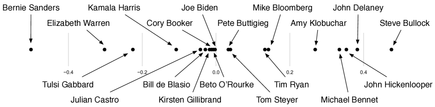
Figure 3: Based on tweets, the tbip places 2020 Democratic presidential candidates along an interpretable progressive-to-moderate spectrum.

Bernie Sanders (I-VT).

Bernie Sanders is an Independent senator who caucuses with the Democratic party; we refer to him as a Democrat. Among Democrats, his ideal point changes the most between one estimated from speeches and one estimated from votes. Although his vote-based ideal point is the 17th most liberal, the tbip ideal point based on Senate speeches is the most extreme.

We use the likelihood ratio to understand this difference in his vote-based and speech-based ideal points. His speeches with the highest likelihood ratio are about income inequality and universal health care, which are both progressive issues. The following is an excerpt from one such speech:

“The United States is the only major country on Earth that does not guarantee health care to all of our people… At a time when the rich are getting richer and the middle class is getting poorer, the Republicans take from the middle class and working families to give more to the rich and large corporations.”

Sanders is considered one of the most liberal senators; his extreme speech ideal point is sensible.

That Sanders’ vote-based ideal point is not more extreme appears to be a limitation of the vote-based method. Applying the likelihood ratio to votes helps illustrate the issue. (Here a bill takes the place of a document.) The ratio identifies H.R. 2048 as influential. This bill is a rollback of the Patriot Act that Sanders voted against because it did not go far enough to reduce federal surveillance capabilities (RealClearPolitics, 2015). In voting “nay”, he was joined by one Democrat and 30 Republicans, almost all of whom voted against the bill because they did not want surveillance capabilities curtailed at all. Vote-based ideal points, which only model binary values, cannot capture this nuance in his opinion. As a result, Sanders’ vote-based ideal point is pulled to the right.

Deb Fischer (R-NE).

Turning to tweets, Deb Fischer’s tweet-based ideal point is more liberal than her vote-based ideal point; her vote ideal point is the 11th most extreme among senators, while her tweet ideal point is the 43rd most extreme. The likelihood ratio identifies the following tweets as responsible for this moderation:

“I want to empower women to be their own best advocates, secure that they have the tools to negotiate the wages they deserve. #EqualPay”

“FACT: 1963 Equal Pay Act enables women to sue for wage discrimination. #GetitRight #EqualPayDay”

The tbip associates terms about equal pay and women’s rights with liberals. A senator with the most liberal ideal point would be expected to use the phrase “#EqualPay” 20 times as much as a senator with the most conservative ideal point and “women” 9 times as much, using the topics in Fischer’s first tweet above. Fischer’s focus on equal pay for women moderates her tweet ideal point.

Ideology Top Words Progressive class, billionaire, billionaires, walmart, wall street, corporate, executives, government Neutral economy, pay, trump, business, tax, corporations, americans, billion Moderate trade war, trump, jobs, farmers, economy, economic, tariffs, businesses, promises, job Progressive #medicareforall, insurance companies, profit, health care, earth, medical debt, health care system, profits Neutral health care, plan, medicare, americans, care, access, housing, millions Moderate healthcare, universal healthcare, public option, plan, universal coverage, universal health care, away, choice Progressive green new deal, fossil fuel industry, fossil fuel, planet, pass, #greennewdeal, climate crisis, middle ground Neutral climate change, climate, climate crisis, plan, planet, crisis, challenges, world Moderate solutions, technology, carbon tax, climate change, challenges, climate, negative, durable

Table 3: The tbip learns topics from 2020 Democratic presidential candidate tweets that vary as a function of the candidate’s political positions. The neutral topics are for an ideal point of 0; the ideological topics fix ideal points at $-1$ and $+1$. We interpret one extreme as progressive and the other as moderate.

Jeff Sessions (R-AL).

The likelihood ratio can also point to model limitations. Jeff Sessions is a conservative voter, but the tbip identifies his speeches as moderate. One of the most influential speeches for his moderate text ideal point, as identified by the likelihood ratio, criticizes Deferred Actions for Childhood Arrivals (DACA), an immigration policy established by President Obama that introduced employment opportunities for undocumented individuals who arrived as children:

“The President of the United States is giving work authorizations to more than 4 million people, and for the most part they are adults. Almost all of them are adults. Even the so-called DACA proportion, many of them are in their thirties. So this is an adult job legalization program.”

This is a conservative stance against DACA. So why does the tbip identify it as moderate? As depicted in Table 1, liberals bring up “DACA” when discussing immigration, while conservatives emphasize “laws” and “homeland security.” The fitted expected count of “DACA” using the most liberal ideal point for the topics in the above speech is $1.04$, in contrast to $0.04$ for the most conservative ideal point. Since conservatives do not focus on DACA, Sessions even bringing up the program sways his ideal point toward the center. Although Sessions refers to DACA disapprovingly, the bag-of-words model cannot capture this negative sentiment.

5.4 2020 Democratic candidates

We also analyze tweets from Democratic presidential candidates for the 2020 election. Since all of the candidates running for President do not vote on a shared set of issues, their ideal points cannot be estimated using vote-based methods.

Figure 3 shows tweet-based ideal points for the 2020 Democratic candidates. Elizabeth Warren and Bernie Sanders, who are often considered progressive, are on one extreme. Steve Bullock and John Delaney, often considered moderate, are on the other. The selected topics in Table 3 showcase this spectrum. Candidates with progressive ideal points focus on: billionaires and Wall Street when discussing the economy, Medicare for All when discussing health care, and the Green New Deal when discussing climate change. On the other extreme, candidates with moderate ideal points focus on: trade wars and farmers when discussing the economy, universal plans for health care, and technological solutions to climate change.

6 Summary

We developed the text-based ideal point model (tbip), an ideal point model that analyzes texts to quantify the political positions of their authors. It estimates the latent topics of the texts, the ideal points of their authors, and how each author’s political position affects her choice of words within each topic. We used the tbip to analyze U.S. Senate speeches and tweets. Without analyzing the votes themselves, the tbip separates lawmakers by party, learns interpretable politicized topics, and infers ideal points close to the classical vote-based ideal points. Moreover, the tbip can estimate ideal points of anyone who authors political texts, including non-voting actors. When used to study tweets from 2020 Democratic presidential candidates, the tbip identifies them along a progressive-to-moderate spectrum.

Acknowledgments

This work is funded by ONR N00014-17-1-2131, ONR N00014-15-1-2209, NIH 1U01MH115727-01, NSF CCF-1740833, DARPA SD2 FA8750-18-C-0130, Amazon, NVIDIA, and the Simons Foundation. Keyon Vafa is supported by NSF grant DGE-1644869. We thank Voxgov for providing us with senator tweet data. We also thank Mark Arildsen, Naoki Egami, Aaron Schein, and anonymous reviewers for helpful comments and feedback.

Appendix A Algorithm

Input: Word counts $\boldsymbol{y}$, authors $\boldsymbol{a}$, and number of topics $K$ ($D$ documents and $V$ words)

Output: Document intensities $\hat{\boldsymbol{\theta}}$, neutral topics $\hat{\boldsymbol{\beta}}$, ideological topic offsets $\hat{\boldsymbol{\eta}}$, ideal points $\hat{\boldsymbol{x}}$

Pretrain: Hierarchical Poisson factorization (Gopalan et al., 2015) to obtain initial estimates $\hat{\boldsymbol{\theta}}$ and $\hat{\boldsymbol{\beta}}$

Initialize: Variational parameters $\boldsymbol{\sigma}^{2}_{\theta},\boldsymbol{\sigma}^{2}_{\beta},\boldsymbol{\mu}_{\eta},\boldsymbol{\sigma}^{2}_{\eta},\boldsymbol{\mu}_{x},\boldsymbol{\sigma}^{2}_{x}$ randomly, $\boldsymbol{\mu}_{\theta}=\log(\hat{\boldsymbol{\theta}})$, $\boldsymbol{\mu}_{\beta}=\log(\hat{\boldsymbol{\beta}})$

Compute weights $\boldsymbol{w}$ as in Equation 4

while the evidence lower bound (elbo) has not converged do

       sample a document index $d\in\{1,2,\dots,D\}$

       sample $\boldsymbol{z}_{\theta},\boldsymbol{z}_{\beta},\boldsymbol{z}_{\eta},\boldsymbol{z}_{x}\sim\mathcal{N}(\boldsymbol{0},\boldsymbol{I})$

        $\triangleright$ Sample noise distribution

       Set $\tilde{\boldsymbol{\theta}}=\exp(\boldsymbol{z}_{\theta}\odot\boldsymbol{\sigma}_{\theta}+\boldsymbol{\mu}_{\theta})$ and $\tilde{\boldsymbol{\beta}}=\exp(\boldsymbol{z}_{\beta}\odot\boldsymbol{\sigma}_{\beta}+\boldsymbol{\mu}_{\beta})$

        $\triangleright$ Reparameterize

       Set $\tilde{\boldsymbol{\eta}}=\boldsymbol{z}_{\eta}\odot\boldsymbol{\sigma}_{\eta}+\boldsymbol{\mu}_{\eta}$ and $\tilde{\boldsymbol{x}}=\boldsymbol{z}_{x}\odot\boldsymbol{\sigma}_{x}+\boldsymbol{\mu}_{x}$

        $\triangleright$ Reparameterize

       for $v\in\{1,\dots,V\}$ do

             Set $\lambda_{dv}=\left(\sum_{k}\tilde{\theta}_{dk}\tilde{\beta}_{kv}\exp(\tilde{\eta}_{kv}\tilde{x}_{a_{d}})\right)*w_{a_{d}}$

             Compute $\log p(y_{dv}|\tilde{\boldsymbol{\theta}},\tilde{\boldsymbol{\beta}},\tilde{\boldsymbol{\eta}},\tilde{\boldsymbol{x}})=\log\text{Pois}(y_{dv}|\lambda_{dv})$

              $\triangleright$ Log-likelihood term

            

       end for

      Set $\log p(\boldsymbol{y}_{d}|\tilde{\boldsymbol{\theta}},\tilde{\boldsymbol{\beta}},\tilde{\boldsymbol{\eta}},\tilde{\boldsymbol{x}})=\sum_{v}\log p(y_{dv}|\tilde{\boldsymbol{\theta}},\tilde{\boldsymbol{\beta}},\tilde{\boldsymbol{\eta}},\tilde{\boldsymbol{x}})$

        $\triangleright$ Sum over words

       Compute $\log p(\tilde{\boldsymbol{\theta}},\tilde{\boldsymbol{\beta}},\tilde{\boldsymbol{\eta}},\tilde{\boldsymbol{x}})$ and $\log q(\tilde{\boldsymbol{\theta}},\tilde{\boldsymbol{\beta}},\tilde{\boldsymbol{\eta}},\tilde{\boldsymbol{x}})$

        $\triangleright$ Prior and entropy terms

       Set $\lx@glossaries@gls@link{acronym}{ELBO}{\leavevmode{\color[rgb]{0,0,0}\textsc{elbo}}}=\log p(\tilde{\boldsymbol{\theta}},\tilde{\boldsymbol{\beta}},\tilde{\boldsymbol{\eta}},\tilde{\boldsymbol{x}})+N*\log p(\boldsymbol{y}_{d}|\tilde{\boldsymbol{\theta}},\tilde{\boldsymbol{\beta}},\tilde{\boldsymbol{\eta}},\tilde{\boldsymbol{x}})$

       $\ \ \ \ \ \ \ \ \ \ \ \ \ \ \ \ \ \ \ \ \ -\log q(\tilde{\boldsymbol{\theta}},\tilde{\boldsymbol{\beta}},\tilde{\boldsymbol{\eta}},\tilde{\boldsymbol{x}})$

       Compute gradients $\nabla_{\phi}\lx@glossaries@gls@link{acronym}{ELBO}{\leavevmode{\color[rgb]{0,0,0}\textsc{elbo}}}$ using automatic differentiation

       Update parameters $\phi$

      

end while

return approximate posterior means $\hat{\boldsymbol{\theta}},\hat{\boldsymbol{\beta}},\hat{\boldsymbol{\eta}},\hat{\boldsymbol{x}}$

Algorithm 1 The tbip

We present the full procedure for training the text-based ideal point model (tbip) in Algorithm 1. We make a final modification to the model in Equation 3. If some political authors are more verbose than others (i.e. use more words per document), the learned ideal points may reflect verbosity rather than a political preference. Thus, we multiply the expected word count by a term that captures the author’s verbosity compared to all authors. Specifically, if $n_{s}$ is the average word count over documents for author $s$, we set a weight:

$$w_{s}=\frac{n_{s}}{\frac{1}{S}\sum_{s^{\prime}}n_{s^{\prime}}},$$ (4)

for $S$ the number of authors. We then multiply the rate in Equation 3 by $w_{a_{d}}$. Empirically, we find this modification does not make much of a difference for the correlation results, but it helps us interpret the ideal points for the qualitative analysis.

Appendix B Data and inference settings

Senator speeches

We remove senators who made less than 24 speeches. To lessen non-ideological correlations in the speaking patterns of senators from the same state, we remove cities and states in addition to stopwords and procedural terms. We include all unigrams, bigrams, and trigrams that appear in at least 0.1% of documents and at most 30%. To ensure that the inferences are not influenced by procedural terms used by a small number of senators with special appointments, we only include phrases that are spoken by 10 or more senators. This preprocessing leaves us with 19,009 documents from 99 senators, along with 14,503 terms in the vocabulary.

To train the tbip, we perform stochastic gradient ascent using Adam (Kingma and Ba, 2015), with a mini-batch size of 512. To curtail extreme word count values from long speeches, we take the natural logarithm of the counts matrix before performing inference (appropriately adding 1 and rounding so that a word count of 1 is transformed to still be 1). We use a single Monte Carlo sample to approximate the gradient of each batch. We assume 50 latent topics and posit the following prior distributions: $\theta_{dk},\beta_{kv}\sim\text{Gamma}(0.3,0.3)$, $\eta_{kv},x_{s}\sim\mathcal{N}(0,1)$.

We train the vote ideal point model by removing all votes that are not cast as “yea” or “nay” and performing mean-field variational inference with Gaussian variational distributions. Since each variational family is Gaussian, we approximate gradients using the reparameterization trick (Rezende et al., 2014; Kingma and Ba, 2015).

	Speeches 111		Speeches 112		Speeches 113		Tweets 114
	Corr.	SRC	Corr.	SRC	Corr.	SRC	Corr.	SRC
wordfish	0.52	0.49	0.51	0.51	0.71	0.65	0.79	0.74
wordshoal	0.62	0.66	0.58	0.51	0.46	0.46	—	—
tbip	0.82	0.77	0.85	0.85	0.89	0.86	0.94	0.88

Table 4: The tbip learns ideal points most similar to dw-nominate vote ideal points for U.S. senator speeches and tweets. It learns closer ideal points than wordfish and wordshoal in terms of both correlation (Corr.) and Spearman’s rank correlation (SRC). The numbers in the column titles refer to the Senate session of the corpus. wordshoal cannot be applied to tweets because there are no debate labels.

For the comparisons against wordfish and wordshoal, we preprocess speeches in the same way as Lauderdale and Herzog (2016a). We train each Senate session separately, thereby only including one timestep for wordfish. For this reason, our results on the U.S. Senate differ from those reported by Lauderdale and Herzog (2016a), who train a model jointly over all time periods. Additionally, we use variational inference with reparameterization gradients to train all methods. Specifically, we perform mean-field variational inference, positing Gaussian variational families on all real variables and lognormal variational families on all positive variables.

Senator tweets

Our Senate tweet preprocessing is similar to the Senate speech preprocessing, although we now include all terms that appear in at least 0.05% of documents rather than 0.01% to account for the shorter tweet lengths. We remove cities and states in addition to stopwords and the names of politicians. This preprocessing leaves us with 209,779 tweets. We use the same model and hyperparameters as for speeches, although we no longer take the natural logarithm of the counts matrix since individual tweets cannot have extreme word counts due to the character limit. We use a batch size of 1,024.

2020 Democratic candidates

We scrape the Twitter feeds of 19 candidates, including all tweets between January 1, 2019 and February 27, 2020. We do not include Andrew Yang, Jay Inslee, and Marianne Williamson since it is difficult to define the political preferences of non-traditional or single-issue candidates. We follow the same preprocessing we used for the 114th Senate, except we include tokens that are used in more than 0.05% of documents rather than 0.1%. We remove phrases used by only one candidate, along with stopwords and candidate names. This preprocessing leaves us with 45,927 tweets for the 19 candidates. We use the same model and hyperparameters as for senator tweets.

Appendix C Comparison to DW-Nominate

dw-nominate (Poole, 2005) is a dynamic method for learning ideal points from votes. As opposed to the vote ideal point model in Section 2.1, it analyzes votes across multiple Senate sessions. It also learns two latent dimensions per legislator. We also compare text ideal points to the first dimension of DW-Nominate, which corresponds to economic/redistributive preferences (Lewis et al., 2020). We use the fitted dw-nominate ideal points available on Voteview (Lewis et al., 2020). The tbip learns ideal points closer to dw-nominate than wordfish and wordshoal; see Table 4.

In Section 5, we observed that Bernie Sanders’ vote ideal point is somewhat moderate under the scalar ideal point model from Section 2.1. It is worth noting that Sanders’ vote ideal point is more extreme under dw-nominate than under the scalar model: his dw-nominate ideal point is the third-most extreme among Democrats. Since dw-nominate uses two dimensions to model each legislator’s latent preferences, it can more flexibly model Sanders’ voting deviations. Additionally, the dynamic nature of dw-nominate may capture salient information from other Senate sessions. However, restricting the vote ideal point to be static and a scalar, like it is for the tbip, results in the more moderate vote ideal point in Section 5.

References

- Bailey (2001) Michael Bailey. 2001. Ideal point estimation with a small number of votes: A random-effects approach. Political Analysis, 9(3):192–210.
- Baumer et al. (2015) Eric Baumer, Elisha Elovic, Ying Qin, Francesca Polletta, and Geri Gay. 2015. Testing and comparing computational approaches for identifying the language of framing in political news. In Proceedings of ACL.
- Baumgartner et al. (2008) Frank R Baumgartner, Suzanna L De Boef, and Amber E Boydstun. 2008. The decline of the death penalty and the discovery of innocence. Cambridge University Press.
- Benoit and Laver (2003) Kenneth Benoit and Michael Laver. 2003. Estimating Irish party policy positions using computer wordscoring: The 2002 election. Irish Political Studies, 18(1):97–107.
- Blei et al. (2017) David M Blei, Alp Kucukelbir, and Jon D McAuliffe. 2017. Variational inference: A review for statisticians. Journal of the American Statistical Association, 112(518):859–877.
- Bock and Aitkin (1981) R Darrell Bock and Murray Aitkin. 1981. Marginal maximum likelihood estimation of item parameters: Application of an EM algorithm. Psychometrika, 46(4):443–459.
- Canny (2004) John Canny. 2004. GaP: A factor model for discrete data. In ACM SIGIR Conference on Research and Development in Information Retrieval.
- Card et al. (2015) Dallas Card, Amber Boydstun, Justin H Gross, Philip Resnik, and Noah A Smith. 2015. The media frames corpus: Annotations of frames across issues. In Proceedings of ACL.
- Cemgil (2009) Ali Taylan Cemgil. 2009. Bayesian inference for nonnegative matrix factorisation models. Computational Intelligence and Neuroscience, 2009.
- Chong and Druckman (2007) Dennis Chong and James N Druckman. 2007. Framing theory. Annual Review of Political Science, 10:103–126.
- Clinton et al. (2004) Joshua Clinton, Simon Jackman, and Douglas Rivers. 2004. The statistical analysis of roll call data. American Political Science Review, 98(2):355–370.
- Entman (1993) Robert M Entman. 1993. Framing: Toward clarification of a fractured paradigm. Journal of Communication, 43(4):51–58.
- Gentzkow et al. (2018) Matthew Gentzkow, Jesse M Shapiro, and Matt Taddy. 2018. Congressional record for the 43rd-114th Congresses: Parsed speeches and phrase counts. Stanford Libraries.
- Gentzkow et al. (2019) Matthew Gentzkow, Jesse M Shapiro, and Matt Taddy. 2019. Measuring group differences in high-dimensional choices: Method and application to congressional speech. Econometrica, 87(4):1307–1340.
- Gerrish and Blei (2011) Sean Gerrish and David M Blei. 2011. Predicting legislative roll calls from text. In Proceedings of ICML.
- Gerrish and Blei (2012) Sean Gerrish and David M Blei. 2012. How they vote: Issue-adjusted models of legislative behavior. In Proceedings of NeurIPS.
- Gopalan et al. (2015) Prem Gopalan, Jake M Hofman, and David M Blei. 2015. Scalable recommendation with Poisson factorization. In Proceedings of UAI.
- Gopalan et al. (2014) Prem K Gopalan, Laurent Charlin, and David M Blei. 2014. Content-based recommendations with Poisson factorization. In Proceedings of NeurIPS.
- Herzog and Benoit (2015) Alexander Herzog and Kenneth Benoit. 2015. The most unkindest cuts: Speaker selection and expressed government dissent during economic crisis. The Journal of Politics, 77(4):1157–1175.
- Ho et al. (2008) Daniel E Ho, Kevin M Quinn, et al. 2008. Measuring explicit political positions of media. Quarterly Journal of Political Science, 3(4):353–377.
- Hoffman et al. (2013) Matthew D Hoffman, David M Blei, Chong Wang, and John Paisley. 2013. Stochastic variational inference. The Journal of Machine Learning Research, 14(1):1303–1347.
- Imai et al. (2016) Kosuke Imai, James Lo, and Jonathan Olmsted. 2016. Fast estimation of ideal points with massive data. American Political Science Review, 110(4):631–656.
- Iyyer et al. (2014) Mohit Iyyer, Peter Enns, Jordan Boyd-Graber, and Philip Resnik. 2014. Political ideology detection using recursive neural networks. In Proceedings of ACL.
- Jackman (2001) Simon Jackman. 2001. Multidimensional analysis of roll call data via Bayesian simulation: Identification, estimation, inference, and model checking. Political Analysis, 9(3):227–241.
- Johnson et al. (2017) Kristen Johnson, Di Jin, and Dan Goldwasser. 2017. Leveraging behavioral and social information for weakly supervised collective classification of political discourse on Twitter. In Proceedings of ACL.
- Jordan et al. (1999) Michael I Jordan, Zoubin Ghahramani, Tommi S Jaakkola, and Lawrence K Saul. 1999. An introduction to variational methods for graphical models. Machine Learning, 37(2):183–233.
- Kim et al. (2018) In Song Kim, John Londregan, and Marc Ratkovic. 2018. Estimating spatial preferences from votes and text. Political Analysis, 26(2):210–229.
- Kingma and Ba (2015) Diederik P Kingma and Jimmy Ba. 2015. Adam: A method for stochastic optimization. In Proceedings of ICLR.
- Kingma and Welling (2014) Diederik P Kingma and Max Welling. 2014. Auto-encoding variational Bayes. In Proceedings of ICLR.
- Lauderdale and Clark (2014) Benjamin E Lauderdale and Tom S Clark. 2014. Scaling politically meaningful dimensions using texts and votes. American Journal of Political Science, 58(3):754–771.
- Lauderdale and Herzog (2016a) Benjamin E Lauderdale and Alexander Herzog. 2016a. Measuring political positions from legislative speech. Political Analysis, 24(3):374–394.
- Lauderdale and Herzog (2016b) Benjamin E Lauderdale and Alexander Herzog. 2016b. Replication data for: Measuring political positions from legislative speech. Harvard Dataverse.
- Laver et al. (2003) Michael Laver, Kenneth Benoit, and John Garry. 2003. Extracting policy positions from political texts using words as data. American Political Science Review, 97(2):311–331.
- Lee and Seung (1999) Daniel D Lee and H Sebastian Seung. 1999. Learning the parts of objects by non-negative matrix factorization. Nature, 401(6755):788.
- Lewis et al. (2020) Jeffrey B. Lewis, Keith Poole, Howard Rosenthal, Adam Boche, Aaron Rudkin, and Luke Sonnet. 2020. Voteview: Congressional roll-call votes database.
- Lo et al. (2016) James Lo, Sven-Oliver Proksch, and Jonathan B Slapin. 2016. Ideological clarity in multiparty competition: A new measure and test using election manifestos. British Journal of Political Science, 46(3):591–610.
- Lowe (2008) Will Lowe. 2008. Understanding wordscores. Political Analysis, 16(4):356–371.
- Martin and Quinn (2002) Andrew D Martin and Kevin M Quinn. 2002. Dynamic ideal point estimation via Markov Chain Monte Carlo for the US Supreme Court, 1953–1999. Political Analysis, 10(2):134–153.
- McCarty et al. (1997) Nolan M McCarty, Keith T Poole, and Howard Rosenthal. 1997. Income redistribution and the realignment of American politics. American Enterprise Institute Press.
- Nguyen et al. (2015) Viet-An Nguyen, Jordan Boyd-Graber, Philip Resnik, and Kristina Miler. 2015. Tea Party in the house: A hierarchical ideal point topic model and its application to Republican legislators in the 112th Congress. In Proceedings of ACL.
- Poole (2005) Keith T Poole. 2005. Spatial models of parliamentary voting. Cambridge University Press.
- Poole and Rosenthal (1985) Keith T Poole and Howard Rosenthal. 1985. A spatial model for legislative roll call analysis. American Journal of Political Science, pages 357–384.
- Poole and Rosenthal (2000) Keith T Poole and Howard Rosenthal. 2000. Congress: A political-economic history of roll call voting. Oxford University Press on Demand.
- Proksch and Slapin (2009) Sven-Oliver Proksch and Jonathan B Slapin. 2009. How to avoid pitfalls in statistical analysis of political texts: The case of Germany. German Politics, 18(3):323–344.
- Ranganath et al. (2015) Rajesh Ranganath, Linpeng Tang, Laurent Charlin, and David M Blei. 2015. Deep exponential families. In Proceedings of AISTATS.
- RealClearPolitics (2015) RealClearPolitics. 2015. Bernie Sanders on USA Freedom Act: ”I may well be voting for it,” does not go far enough. Online; posted 31-May-2015.
- Rezende et al. (2014) Danilo Jimenez Rezende, Shakir Mohamed, and Daan Wierstra. 2014. Stochastic backpropagation and approximate inference in deep generative models. In Proceedings of ICML.
- Schwarz et al. (2017) Daniel Schwarz, Denise Traber, and Kenneth Benoit. 2017. Estimating intra-party preferences: Comparing speeches to votes. Political Science Research and Methods, 5(2):379–396.
- Slapin and Proksch (2008) Jonathan B Slapin and Sven-Oliver Proksch. 2008. A scaling model for estimating time-series party positions from texts. American Journal of Political Science, 52(3):705–722.
- Song et al. (2018) Kyungwoo Song, Wonsung Lee, and Il-Chul Moon. 2018. Neural ideal point estimation network. In Thirty-Second AAAI Conference on Artificial Intelligence.
- Tsur et al. (2015) Oren Tsur, Dan Calacci, and David Lazer. 2015. A frame of mind: Using statistical models for detection of framing and agenda setting campaigns. In Proceedings of ACL.
- VoxGovFEDERAL (2020) VoxGovFEDERAL. 2020. U.S. senators tweets from the 114th Congress.
- Wainwright et al. (2008) Martin J Wainwright, Michael I Jordan, et al. 2008. Graphical models, exponential families, and variational inference. Foundations and Trends in Machine Learning, 1(1–2):1–305.