Spectroscopic and asteroseismic analysis of the secondary clump red giant HD 226808.

Abstract

In order to clarify the properties of the secondary clump star HD 226808 (KIC 5307747), we combined four years of data from the Kepler space photometry with the high-resolution spectroscopy of the HERMES spectrograph mounted on the Mercator telescope. The fundamental atmospheric parameters, radial velocities, rotation velocities and elemental abundance for Fe and Li were determined by analyzing line strengths and fitting line profiles, based on a 1D LTE model atmosphere. Secondly, we analyzed photometric light curve obtained by Kepler and we extracted asteroseismic data of this target by using LAURA (Lets Analysis, Use and Report of Asteroseismology), a new seismic tool developed for the study of evolved FGK solar-like stars. We determined the evolutionary status and effective temperature; surface gravity; metallicity, microturbulence and chemical abundances for Li, Ti, Fe, and Ni for HD 226808, by employing spectroscopy, asteroseismic scaling relations and evolutionary structure models built in order to match observed data. Our results also show that an accurate synergy between good spectroscopic analysis and asteroseismology can provide a jump toward understanding evolved stars.

1 Introduction

Red giants are cool evolved stars with an extended convective envelope, which can, as in main sequence solar-like stars, stochastically excite modes of oscillation. This stellar evolutionary phase is well studied from both the observational and the theoretical aspects, but still quite intriguing since, after the exhaustion of H in the core, several structural changes occur in the interior of the star along this phase. In fact, the evolution proceed by fusion of hydrogen in a shell surrounding an inert core of helium, which continues to increase its mass and contracts, while the stellar radius expands. If the stellar core reaches a temperature of $\sim$ 100 million K, the fusion of helium through the triple alpha process can start. However, the initial stellar mass will play a defining role on the evolution of the star after helium begins to burn in the core. Stars with masses below $\sim 1.9M_{\odot}$ develop degenerate helium cores which increase their mass while the H is burning in the shell, until the core reaches a critical mass of $M_{c}\sim 0.47M_{\odot}$.

Figure 1: Observed and synthetics spectra around $C_{2}$ region around $\lambda$ 5086 A of HD 226808 (KIC 5307747) as observed by the MERCATOR telescopes. The observed spectrum is represented by black dots. The synthetic spectra represented by red and blue lines were computed with the same spectroscopic fundamental parameters, $T_{eff}=5065$, $log(g)=2.99$, $[Fe/H]=0.08$ and $V_{t}=1.27$ and presented on the table 2. The synthetic spectrum represented by the red line used $[C/H]=-0,05$; $[Ti/H]=-0,10$; $[Fe/H]=0,01$; $[Ni/H]=0,33$. The synthetic spectrum represented by the blue line used $[C/H]=-0,08$; $[Ti/H]=-0,13$; $[Fe/H]=0,08$; $[Ni/H]=0,36$. The comparison of synthetic and observed spectra results a ”o-c” (difference between the observed and synthetic spectra) of about 0.02 dex for these species.

At this point, a helium flash occurs abruptly in the center of the helium core and the degeneracy is gradually lifted. Those stars, due to the degenerate condition of the core, have similar core masses, hence similar luminosities, and hence are found in a narrow region of a H-R diagram, forming the so-called ‘red clump’ (RC) (e.g., Cannon, 1970; Faulkner & Cannon, 1973; Girardi et al., 1998; Girardi, 1999). On the other hand, stars with masses higher than $\sim 1.9M_{\odot}$ will not develop a degenerate helium core in the post-main sequence phase. They will not have an explosive liberation of energy like the one seen during the helium flash. Instead, they will have a gradual ignition of helium. Therefore, those stars will occupy a region of the H-R diagram similar to the red clump, but at lower luminosities and spread wide. This group, which includes more massive core helium burning stars, at ages of about 1 Gyr, is referred as the secondary clump and its components are the second clump stars (see e.g., Girardi, 1999).

Hawkins et al. (2017) studied in details the spectroscopic signatures of genuine core helium burning red clump giant stars and how they compare to shell hydrogen burning RGB stars. Additionally, spectroscopic study of genuine RGB or RC stars have been done by Anders et al. (2016) for some APOGEE and CoRoT targets. Red clump stars are natural standard candles (Stanek et al., 1998; Hawkins et al., 2017), while regular RGB stars or more massive secondary RC stars of nearly the same effective temperatures ($T_{eff}$) are not. In this context, finding and characterizing core helium burning RC stars is very important to fine tune stellar evolution and Galactic archeology, and consequently for building a precise cosmic distance ladder (Stanek et al., 1998; Bressan et al., 2013; Bovy et al., 2014; Gontcharov, 2017; Hawkins et al., 2017). Distinguish RC stars from less evolved shell hydrogen burning RGB stars or more massive secondary RC stars is a critical point and a bottle neck to solving some stellar astrophysics problems (Bressan et al., 2013).

Fortunately, continuous photometric observations from space missions such as CoRoT (Baglin et al., 2006) and Kepler (Borucki et al., 2009), provide photometric data of an unprecedented quality. This gives us the possibility to better distinguish the evolutionary status of red giants along the H-shell burning phase before He-ignition from those on the He-burning phase after He-ignition, as described by Bedding et al. (2011). In particular, by using asteroseismic scaling relations calibrated on solar values, it has been possible to determine with good accuracy stellar mass ($M$) and radius ($R$) (e.g., Pinsonneault et al., 2014; Casagrande et al., 2014) of hundreds of observed red-giant stars. Several progresses have been made during the last decade and asteroseismology provides a way forward to classify RC based on stellar natural oscillation frequencies. However at present, some RC stars, classified so far as authentic secondary clump giant stars (Mosser et al., 2014), have a high resolution spectroscopic study. Therefore the importance of this analysis.

In this study, we use photometric data from Kepler space telescope and HERMES ground-based high-resolution spectroscopy to produce a deep analysis of the bright red-giant star HD 226808 (KIC 530774). In particular, this star is one of three brightest classified as secondary clump star and observed by Kepler on long cadence mode (Mosser et al., 2014). This paper is organized as follows: in Section 2, we present the spectroscopic observations and spectroscopic derived fundamental parameters. In Section 3 we present asteroseismic analysis. In Section 4 we compare the asteroseismic results with evolutionary models. Conclusions are presented in Section 5.

2 Spectroscopic observations

Our target, the star HD 226808 (KIC 530774), with V $=$ 8.67 mag was observed on 2015 July 3 with the High Efficiency and Resolution Mercator Échelle Spectrograph (HERMES, Raskin et al. 2011; Raskin 2011) mounted on the 1.2 m Mercator Telescope at the Observatorio del Roque de los Muchachos on La Palma, Canary Islands, Spain. The HERMES spectra covers a wavelength range between 375 and 900 nm with a spectral resolution of R$\simeq$85 000. The wavelength reference was obtained from emission spectra of Thorium-Argon-Neon reference frames in close proximity to the individual exposure. The standard steps of the spectral reduction were performed with an instrument-specific pipeline as described by Raskin et al. (2011) and Raskin (2011). The radial velocity (RV) for each individual spectrum was determined from the cross correlation of the stellar spectrum in the wavelength range between 478 and 653 nm with a standard mask optimized for Arcturus provided by the HERMES pipeline toolbox. For HERMES, the 3$\sigma$ level of the night-to-night stability for the observing mode described above is $\sim$300 m/s, which is used as the classical threshold for RV variations to detect binarity. We corrected individual spectra for the Doppler shift before normalization and combined individual spectra as described in Beck et al. (2016). The total integration time was 1.7 hrs, split into four equal parts of 1500 seconds each. The final spectrum, stacked from an individual exposures shows S/N $\simeq$ 150 around the Li i $\lambda$ 670 nm line.

2.1 Fundamental parameters from HERMES spectroscopy

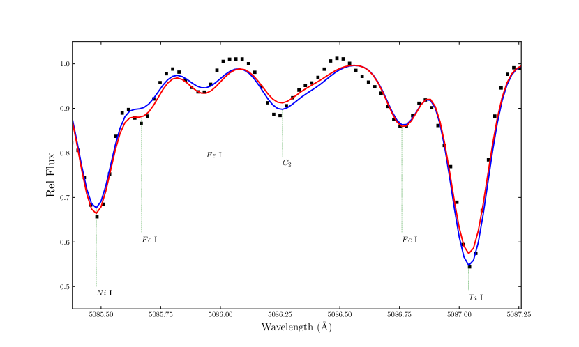
For the fundamental parameters, the analysis of HD 226808 starts by using as a first guess fundamental parameters (effective temperature $T_{\rm eff}$; surface gravity $\log g$; metallicity [Fe/H] and microturbulence) from the revised Kepler Input Catalog (KIC) by Huber et al. (2014). Next, we used the ARES code (v2) (Sousa et al., 2007, 2015) to measure equivalent widths (EW) of selected spectra absorption Fe I and Fe II lines, and with the q2 code Ramírez et al. (2014) we determined the fundamental physical parameters based on a line list, as described by Ramírez et al. (2014). Then, we refine the process based on one-dimensional (1D) local thermodynamic equilibrium (LTE) model atmosphere as described by Beck et al. (2016). We also considered the Arcturus and solar parameters as other reference values, as described by Hinkle & Wallace (2005), Ramírez & Allende Prieto (2011), Meléndez et al. (2012), Monroe et al. (2013), and Ramírez et al. (2014). Final spectroscopic parameters, such as the values of effective temperature $T_{\rm eff}$, surface gravity $\log g$, metallicity $[{\rm Fe/H}]$, and A(Li) of HD 226808 are given in Table 2. Typically, stellar parameters uncertainties were computed as descried by Epstein et al. (2010) and Bensby et al. (2014) and are as ${}^{+39}_{-29}$, $\pm 0.08$, $\pm 0.04$ and $\pm 0.04$ for Teff, log g, [Fe/H], and $V_{\rm t}$, respectively. For abundances determinations, we used spectral synthesis based on a combination of a 2014 version of the code MOOG (Sneden, 1973) with Kurucz atmosphere models (Castelli & Kurucz, 2004) and a line lists as described in the Table 1. (for fundamental parameters determinations, we used a line list as described in the appendix B). A low lithium abundance signature is found for this secondary red clump giant star. However, on the same evolutionary stage, some lithium-rich stars has been found by Bharat Kumar et al. (2018). The values that we obtained for effective temperature and metallicity are comparable with those by Takeda & Tajitsu (2015) who observed this star with the High Dispersion Spectrograph at the Subaru telescope. The value of $\log g$ results to be slightly higher than the value obtained by Takeda & Tajitsu (2015), however within the error bar. In Figure 1 we show part of the spectrum for HD 226808 in the region around 5086 Å. We also show results for two different synthetic spectra computed with the code MOOG for the same spectroscopic fundamental parameters. For the error analysis in the abundances determination we preserve the same fundamental parameters and slightly vary the abundances along a step size from 0.05 until 0.10 dex. The values are shown in the table.

Table 1: Line list used for HD 226808 (KIC 530774).

$wavelength$	$species$	$\chi_{exc}$	$log(gf)$	EW
Å		$eV$		Å
5085.477	28.0	3.658	-1.541	94.12
5085.676	26.0	4.178	-2.610	9.78
5085.837	26.0	4.495	-3.881	9.27
5085.933	26.0	3.943	-3.151	9.77
5086.231	606.0	0.252	-0.110	24.16
5086.251	26.0	4.988	-2.624	24.16
5086.259	606.0	0.252	-0.122	24.16
5086.390	606.0	0.252	-0.133	—
5086.765	25.0	4.435	-1.324	36.07
5086.805	606.0	0.301	-0.649	36.07
5086.997	10108.0	0.040	-10.286	75.40
5087.058	22.0	1.430	-0.780	75.43
5087.065	606.0	0.301	-0.684	75.43

^∗ For species we are using MOOG standard
notation for atomic or molecular identification.
For example, 26 represent Fe(26) while the 0 after
the decimal indicates neutral and 1 singly ionized.
$\chi_{exc}$ is the line excitation potential in electron
volts (eV)

Table 2: Fundamental parameters data of HD 226808 (KIC 530774).

Right Ascension (J2000.0)	$19^{\rm h}57^{\rm m}34.0^{\rm s}$
Declination (J2000.0)	$+40\arcdeg 37\arcmin 16.1\arcsec$
Kp (mag)∗	8.397
spectroscopically derived parameters
Teff (K)	5065 ${}^{+39}_{-29}$
log $g$ (cgs)	$2.99\pm 0.08$
$V_{\rm t}$ (km s-1)	$1.27\pm 0.04$
$[{\rm Fe/H}]{}^{**}$	0.08$~{}\pm~{}$0.04$~{}dex$
$A(Li)$	$\leq$0.58
$A(C)$	8.35 $\pm~{}$0.05$~{}dex$
$A(Ti)$	4.82 $\pm~{}$0.06$~{}dex$
$A(Fe)$	7.58  $\pm~{}$0.07$~{}dex$
$A(Ni)$	6.58 $\pm~{}$0.05$~{}dex$

^∗ Kp is the white light $\it Kepler$ magnitude taken from the
revised Kepler Input Catalog (KIC) (Huber et al., 2014).
^∗∗ Abundances assuming Asplund et al. (2009)

3 Analysis of asteroseismic data

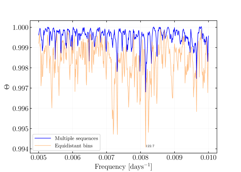
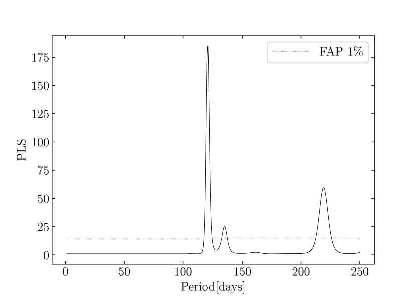
We have developed a code with the purpose of analyzing stellar oscillations and extracting seismic data from light curves. The code makes use of the version 3.6 of the python programming language and has been calibrated by using several stars from the literature, especially the giant stars from Ceillier et al. (2017) and the KIC 4448777 from Di Mauro et al. (2018). The Lets Analysis, Use and Report of Asteroseismology, LAURA (De Moura & De Almeida, 2018), searches the Pre-search Data Conditioning Simple Aperture Photometry, PDC-SAP FLUX light curves retrieved from Mikulski Archive for Space Telescopes, MAST or Kepler Asteroseismic Science Operations Center, KASOC databases and concatenates them in order to reduce noise in the data by using a high rate of oversample to maintain temporal stability by increasing the resolution of the points. After that, the code proceeds to do a clean-up of excessive high values of frequencies thanks to a box-car type filter of 2$\mu$Hz. The time series extracted can then be treated by employing two different tools in order to characterize the periodicity of the star: Lomb-Scargle (LS) periodogram (Scargle, 1982) and minimization of phase dispersion (PDM) (Stellingwerf, 1978). Figure 2 shows the results obtained for the star HD 226808 (KIC 5307747) by using the method of minimization of phase dispersion and showing that the smallest phase occurs for a rotation period of 122 days, in good agreement with the result obtained by Lomb-Scargle periodogram shown in Figure 3. Our method based on the use of LS and PDM together, has given results consistent with the values found by Ceillier et al. (2017) who applied a different technique to a set of red giants, confirming the potential of our tool to determine the rotational period. The main packages of the code are presented in detail in Appendix A.

Figure 2: Determination of the period of rotation of HD 226808 (KIC 5307747) by phase dispersion minimization. The phase is modulated in the minimization of the phase graph by frequency. The smallest phase, for this modulation occurs around 0.008 which represents about 122 days. The check is made by general variance and equidistant or by multiple sequences represented by the two colors.

Figure 3: Lomb-Scargle periodogram of HD 226808 (KIC 5307747). The red line represents the 1% probability limit of the signal. The highest peak indicates rotation.

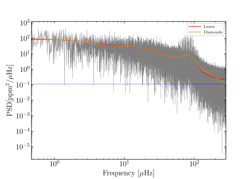
The same code has been implemented to perform the Fast Fourier Transform (FFT) of the time series to analyze the stellar oscillation power spectra and study excess of power at high frequency. The global approach in the seismic study that involves the adjustment of the entire spectrum has challenged us to compare with other already consolidated codes. From that comparison we finally can conclude that LAURA is in good agreement with other ones using similar methods. For example here we show in Figure 4, the comparison of the background modeling methods between LAURA and DIAMONDS (Corsaro et al., 2015) developed for the analysis of HD 226808. We found that the photometric granulation signatures due to intense convective activities on the surface present only subtle differences and do not affect the seismic analysis (Mathur et al., 2011).

Figure 4: LAURA background model represented in comparison to DIAMONDS model by Corsaro et al. (2015) for HD 226808 (KIC 5307747). White noise is shown by blue dashed line. Only subtle differences are present in the region close to the Nyquist frequency (283$\mu$Hz). The gaussian region highlighted in green is similarly analyzed in both.

Figure 5: The gaussian shape of the forest region is shown in dashed green line. The central peak is the $\nu_{max}$ and the others in blue are separated by a periodicity of $\frac{\Delta\nu}{2}$.

Figure 6: The red dot shows the location of HD 226808 in the $logg$ - $T_{eff}$ plane with two evolutionary tracks calculated for increasing values of the mass, while all the other parameters are fixed. The initial helium abundance is $Y_{0}=0.27$, the initial hydrogen abundance $X_{0}=0.71$. The values of the masses are given in the plot. The inset shows the location of the star with two evolutionary tracks obtained by assuming the solar metallicity. Using the metallicity determined by spectroscopy we see that it is a giant of the clump whereas it would be classified as an RGB in the solar metallicity.

3.1 Results

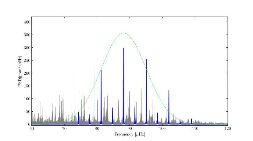
The power spectrum of the light curve for HD 226808 shows a clear excess of power, with a typical Gaussian distribution profile, in the range 60-120 $\mu$Hz due to the radial modes and some additional dipolar and quadrupolar modes, as it is shown in Figure 5. Based on our method, we determined the frequency at maximum oscillation power $\nu_{\rm max}=87.91\pm 1.9\mu$Hz and the so-called large frequency separation between modes with the same harmonic degree $\Delta\nu=6.998\pm 0.06\mu$Hz. The quoted uncertainties are based on a local minimum optimization strategy called the Levenberg-Marquardt method in a specific package, allowing to estimate the following differences:

$$\chi^{2}=\sum_{i}^{N}\frac{[y^{\rm meas}_{i}-y_{i}^{\rm model}]^{2}}{\epsilon_{i}^{2}}$$ (1)

where $y_{i}^{\rm meas}$, $y_{i}^{\rm model}$ and $\epsilon_{i}$ are the set of measured data, the model calculation and estimated uncertainty in the data, respectively. Using the universal method for red-giant oscillation pattern by Mosser et al. (2011) and Mosser et al. (2017) it was possible to identify pure-pressure modes and the identification of several dipole modes by grid-search allowed us to estimate the period spacing $\Delta\Pi=296.85\pm 6.53$s, which places this star on the secondary clump red-giant phase (Mosser et al., 2014). The asteroseismic fundamental parameters found here agree with the results published by Mosser et al. (2012, 2014), who found for this star $\nu_{\rm max}=88.2\mu$Hz, and $\Delta\Pi=296.3\pm 5.9$s, while their large separation, which is $\Delta\nu=6.88\pm 0.05\mu$Hz well agrees within the errors. Table 3 lists the final set of frequencies for the detected individual modes together with their uncertainties.

$l$	$\nu_{n,l}$
0	66.34916 $\pm$ 0.3364
0	73.23633 $\pm$ 0.0292
0	80.02904 $\pm$ 0.2785
0	93.56723 $\pm$ 0.0614
1	62.81494 $\pm$ 0.0205
1	63.38166 $\pm$ 0.0194
1	68.50571 $\pm$ 0.0305
1	75.96745 $\pm$ 0.0583
1	76.06977 $\pm$ 0.0306
1	80.02891 $\pm$ 0.0415
1	82.29577 $\pm$ 0.0455
1	83.05140 $\pm$ 0.0865
1	83.22456 $\pm$ 0.0147
1	83.35049 $\pm$ 0.0611
1	89.19081 $\pm$ 0.0136
1	89.87559 $\pm$ 0.0550
1	90.06449 $\pm$ 0.0399
1	96.03074 $\pm$ 0.0325
2	72.31541 $\pm$ 0.3473
2	79.10025 $\pm$ 0.0461
2	92.04025 $\pm$ 0.1325
3	67.30144 $\pm$ 0.0958
3	74.47983 $\pm$ 0.0431
3	87.91571 $\pm$ 0.0326

Table 3: Frequencies and harmonic degree for observed oscillation modes found using LAURA script. Uncertainties are measured by Lorentzian $(l=0,2,3$) and sinc fits ($l=1$).

3.2 Fundamental parameters from asteroseismic scaling laws

The asteroseismic surface gravity, stellar mass and radius for this star was obtained from the observed $\Delta\nu$ and $\nu_{\mathrm{max}}$ together with the spectroscopic value of $T_{\mathrm{eff}}=5065^{+39}_{-29}\$ following the scaling relations calibrated on solar values as provided by (Kjeldsen & Bedding, 1995; Kallinger et al., 2010; Belkacem et al., 2011):

$$\frac{g_{ast}}{g_{\odot}}\simeq\Bigl{(}\frac{\nu_{max}}{\nu_{max\odot}}\Bigr{)}\Bigl{(}\frac{T_{eff}}{T_{eff\odot}}\Bigr{)}^{1/2}$$ (2)

,

$$\frac{R_{ast}}{R_{\odot}}\simeq\Bigl{(}\frac{\nu_{max}}{\nu_{max\odot}}\Bigr{)}\Bigl{(}\frac{\Delta\nu}{\Delta\nu_{\odot}}\Bigr{)}^{-2}\Bigl{(}\frac{T_{eff}}{T_{eff\odot}}\Bigr{)}^{1/2}$$ (3)

and

$$\frac{M_{ast}}{M_{\odot}}\simeq\Bigl{(}\frac{\nu_{max}}{\nu_{max\odot}}\Bigr{)}^{3}\Bigl{(}\frac{\Delta\nu}{\Delta\nu_{\odot}}\Bigr{)}^{-4}\Bigl{(}\frac{T_{eff}}{T_{eff\odot}}\Bigr{)}^{3/2},$$ (4)

where the values for the Sun are $\Delta\nu_{\odot}=134.9~{}\mu$Hz, $\nu_{max\odot}=3100~{}\mu$Hz and $T_{eff\odot}=5777~{}K$. We obtained that $g_{ast}/g_{\odot}=0.027\pm 0.003$, $M_{ast}/M_{\odot}=2.59\pm 0.24$ and $R_{ast}/R_{\odot}=9.86\pm 0.613$.

In comparison, the ratio $g_{spec}/g_{\odot}$ obtained in the spectroscopic analysis a value of $\sim$0.036. These values agree within the errors from asteroseismic radius and mass values computed by Mosser et al. (2012) and Takeda & Tajitsu (2015) and based on different estimations of maximum power frequency.

4 Comparison with evolutionary models

Given the identified pulsation frequencies and the basic atmospheric parameters, we faced the theoretical challenge to interpret the observed oscillation modes by constructing stellar models which satisfy the spectroscopic and asteroseismic observational constraints. We assumed the effective temperature and surface gravity as calculated in Section 2.1, respectively $T_{\rm eff}=5065^{+34}_{-29}$K, $\log g=2.99\pm 0.08$ dex and metallicity $[Fe/H]=0.08\pm 0.04$, as reported in (Table 2).

We computed theoretical evolutionary models representative of the present star by using the MESA evolutionary code (Paxton et al., 2011), in which we varied the stellar mass and the initial chemical composition in order to match the fundamental parameters available.

Figure 7: Echelle diagram for the star HD 226808. The frequencies of observed modes with $l$ = 0, 1, 2, and 3 and their uncertainties are depicted in blue, red, green and orange, respectively. Open symbols are the oscillation frequencies of our best-fitted model.

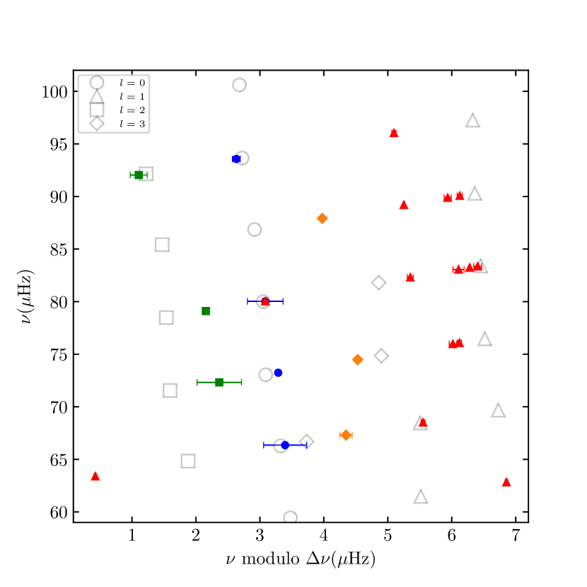
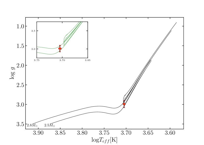
Figure 6 shows two evolutionary tracks obtained with masses $2.5M_{\odot}$ and $2.8M_{\odot}$ and fixed initial composition. We used initial helium abundance of $Y_{0}=0.27$ and initial hydrogen abundance $X_{0}=0.71$ as input to the MESA and plotted in a effective temperature-gravity evolutionary diagram. The location of HD 226808 indicated in Figure 6, which identifies this star in the CHeB phase of evolution (see Section. 1) with a mass between $2.5-2.8M_{\odot}$. We point out that the location of evolutionary tracks in the diagram strongly depends on the metallicity of the model, since it influences the opacity and thus the depth of the convective envelope. If a solar metallicity would have been assumed instead, as we can see in the insert in Figure 6, the star would have appeared to be in the RGB phase, burning hydrogen in a shell around the inert He core. As a result, a good determination of the measured metallicity is essential to achieve a correct determination of the evolutionary status of stars located in this region of the HR diagram. The $A(Li)$ also confirm the evolved status of this star.

Figure 8: Top: difference between frequencies taken from LAURA without any surface correction and those modeled using GYRE. Bottom: Application of surface corrections in order to reduce the differences shown on the top panel. Circles, triangles, squares and diamonds represent the modes $l=0,1,2,3$ , respectively.

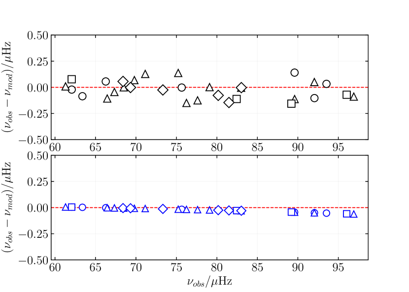
In order to investigate the observed solar-like oscillations, we used the GYRE package (Townsend & Teitler, 2013) to compute adiabatic oscillation frequencies with degree $l=0,1,2,3$ for some of the models satisfying the spectroscopic constraints. In Figure 7, the open symbols represent the best output of the frequency model. Theoretical oscillation frequencies have been corrected by a near-surface effects term following the approach proposed by Ball & Gizon (2014), which has been proved to work much better for evolved stars than other prescriptions. The adjust of the frequencies by a corrective term is a common procedure used for evolved stellar models to overcome the lack of a proper theory for the description of oscillations in the upper surface layers, where frequencies behaviors deviate from the adiabatic assumption. In Figure 8 shows the difference between modelled and observed frequencies for our best model with and without surface corrections, demonstrating the importance of such corrections. Among our models we selected one that appeared to best fit the observed frequencies of HD 226808, and whose characteristics are given in Table 4. This model is characterized by an age of $0.69$ Gyr, a mass $M=2.6\,M_{\odot}$, a radius $R=9.74{R}_{\odot}$. The value of the radius obtained by direct modelling of individual frequencies is now better constrained and well agrees within the error bars obtained by using scaling relation. Furthermore, the value of the mass derived from evolutionary track resulted to be in good agreement with respect to the seismic value, obtained by using the scaling relation and estimated in Section 3.2. Large discrepancies by up to $50\%$ between masses inferred from both methods was pointed out by Miglio et al. (2012) and Takeda & Tajitsu (2015), who explored large sets of red-clump stars, and attributed to the overlapping of the evolutionary tracks of RG stars, with higher masses, and RC stars, with lower masses, at the same clump region of the HR diagram. This difference does not appear in the case of H-shell burning red giants.

Table 4: Parameters of the best model using MESA for HD 226808 (KIC 5307747).

Parameters	Best model
$M/M_{\odot}$	2.60
$R/R_{\odot}$	9.74
$A(Li)$	0.58
$\log T_{eff}$	3.695
$\log g$ (cgs)	2.856
Age (Gyr)	0.69
$\Delta P$(s)	221

Several tests considering interferometry (e.g., Huber et al., 2012; White et al., 2013), Hipparcos parallaxes (Silva Aguirre et al., 2012), eclipsing binaries (e.g., Frandsen et al., 2013; Huber, 2015; Gaulme et al., 2016) and open clusters (e.g., Miglio et al., 2012, 2016; Stello et al., 2016), have demonstrated that mass estimates from asteroseismic scaling relations are accurate to a few percent for main-sequence stars, while larger discrepancies have been identified for evolved stars. Theoretical studies have suggested corrections to scaling relations, for example by comparing the large frequency separation ($\Delta\nu$) calculated from individual frequencies with models (e.g., Stello et al., 2009; White et al., 2011; Guggenberger et al., 2016; Sharma et al., 2016) or an extension of the asymptotic relation (Mosser et al., 2013). For the moment, it remains clear that scaling relation corrections should mainly depend on $T_{eff}$ and evolutionary state. However, it is yet unclear how these corrections should be applied in the case of red clump stars (e.g., Miglio et al., 2012; Sharma et al., 2016).

5 Conclusion

In this study we perform an asteroseismic analysis of the red giant clump star HD 226808 (KIC 530774) based on its high-precision space photometry and high-resolution ground spectroscopic observations. The spectroscopic analysis was important to understand the metallicity of the star, which as discussed in Section 4, has an impact on the evolutionary state of the star. Abundances obtained from the fundamental parameters solution, as for example $A(Li)$, produced good agreement between observational and synthesized values. We used the Kepler photometric data as input to seismic diagnostic tools. We characterized the internal structure and evolutionary status of this secondary clump red giant star, and studied its frequencies, especially since this stars it is one of the brightest star of the Kepler field. We have shown that accurate mass determination of RC stars with such a good agreement between methods is possible. The metallicity effect on oscillation modes for this class of stars is still poorly understood. Future developments will be welcome to better understand this point, especially when comparing giants with very close evolutionary states. Finally, the presented method is robust enough to conduct seismic characterization of giants and and to obtain measurements of rotational period. Our tools are open source and ready for use.

Appendix A Master-Laura

A.1 The algorithm

LAURA (Lets Analysis, Use and Report of Asteroseismology) is written in Python 3 with 5 different packages to download, reduce and analyze raw light curves under the asteroseismology theory. The code uses an object oriented approach and can be easily used even for non-experts in program language. All the additional python packages that we use are free and easy to install using the pip package. Our code is summarized in only 2 files: $LAURA\_master.py$ and $LAURA\_aux.py$. From the $LAURA\_master.py$ file, the user can do all steps to download, reduce and analyze the light curve.

A.2 Installation

In order to use our code, make sure you have python 3.x installed with the follow packages: Astropy (Astropy Collaboration et al., 2013), Scipy (Jones et al., 2001), kplr (Foreman-Mackey, 2018), peakutils (Negri & Vestri, 2017), and lmfit (Newville et al., 2018). Installing the necessary packages in Ubuntu GNU/Linux are done using the follow:

⬇

sudo apt-get install build-essential

sudo apt-get install python3

sudo apt-get install python3-pip

sudo pip install numpy

sudo pip install matplotlib

sudo pip install scipy

sudo pip install astropy

sudo pip install kplr

sudo pip install peakutils

sudo pip install lmfit

Download our source code from GitHub and add the path of where you want to install LAURA. In bash:

⬇

export PYTHONPATH=/home/USER_NAME/LAURA-1.0.0/source:$PYTHONPATH

Add this command to your /.bashrc file or similar (/.cshrc, /.bashrc, /.profile). Go to your LAURA folder and run the checkme.py file to verify if everything is in order. You should get a ”good to go!” message. The installation in a OSX system can be done using Macports and more details can be found in the github guide.

A.3 Packages

LAURA runs from the box with 5 principal packages from the acquisition of the light curve to the Echelle diagram as follows:

⬇

import LAURA_aux as aux

aux.TS_PS(ID,Qtin,Qtfin,cleaning,oversample,path = ’TEMP/’)

aux.FIT_PS(ID)

aux.LS(ID,kernerforca,Pbeg,Pend,PeriodMod,path=’TEMP/’)

aux.OBS(ID)

aux.MOD(ID, largeSep,smallSep,size,Radial_Orders=5)

aux.ECHELLE(ID, deltav)

print (’Done!’)

All parameters configurations can be done using this file. The $TS\_PS$ package get the light curve, cleaning it and create the power spectrum using the time series analysis data. The input parameters are:

• ID: Identification number of star

• Qtin: Inicial quarter for Kepler objects

• Qtfin: Final quarter for Kepler objects

• cleaning: Cleaning parameter for systematic errors

• Oversample: The resolution of the power spectrum

• Path: The folder in which the .fits files will be download

When running this package, LAURA will download all the .fits files from all the quarters you select. If you already have this object in you computer, the code will not download again. A power spectrum will be generated and all files will be store in a folder with the name of the object.

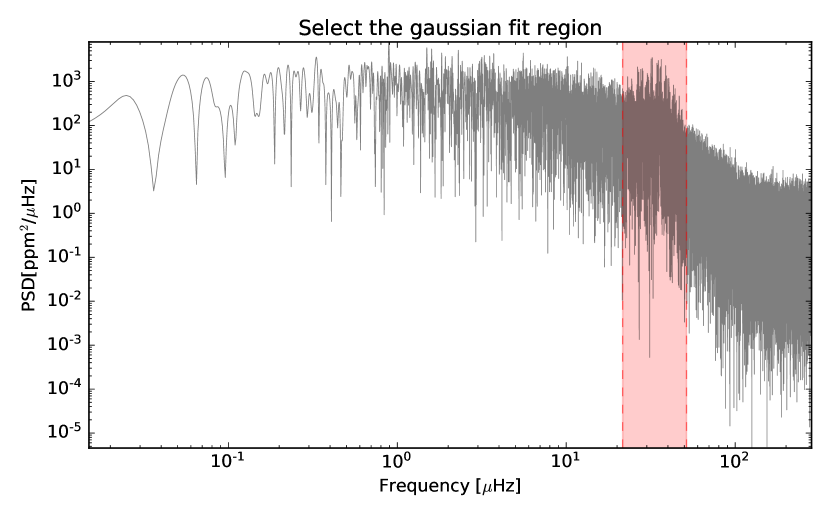
The $FIT\_PS$ package fits a background tendency to the power spectrum generated earlier using only the ID of the object. The first plot will ask you to select the region to fit a Gaussian curve as shown in the Figure 9 following the equation A1

$$f(x)=\frac{A}{\sigma\sqrt{2\pi}}e^{-\frac{(x-\mu)^{2}}{2\sigma^{2}}}$$ (A1)

Where $A$ ins the amplitude, $\mu$ is the center and $\sigma$ is sigma.

Figure 9: Power spectrum of KIC 5006817. The light-red region is the selection to fit a Gaussian fit.

Then, you will be ask to select two consecutive lorentzian fits by clicking the regions of interest. Each click store a position to use as parameters of the following function:

$$f(x)=\frac{A}{\pi}\left(\frac{\sigma}{(x-\mu)^{2}+\sigma^{2}}\right)$$ (A2)

All 3 models (one Gaussian and two Lorentzian) are then use to create a background fit for the power spectrum as shown in the Figure 4.

The $LS$ package run a kernel to smooth out the light curve and run a periodgram either using Lomb Scargle or Phase Dispersion Minimization (PDM). The input parameters are:

• ID: Identification number of star

• Kernel: Strengh of the Gaussian 1D kernel

• Pin: Initial period of search

• Pend: Final period of search

• PeriodMod: Either LS (Lomb Scargle) or PDM (Phase Dispersion Minimization)

• Path: Where to save the data

This package will save all statistical results in a file named $kic\_periodgram.txt$.

The $OBS$ package return all the observed modes from the high frequency region knowing only the ID of the object. First, the user will be asked to select the high frequencies region from the power spectrum. Then it can be select the value of the threshold and the strength of the box kernel. The code then select all the peaks using a Lorentzian peak selector and saves all the output data to the $\_data\_mods\_obs.txt$.

The $MOD$ package makes use of the universal pattern Mosser et al. (2012) to model the possible frequencies of the pure pressure modes of spherical degrees for a defined range of radial orders. It takes as input:

• ID: Identification number of star

• LargeSep: large Frequency separation

• SmallSep: small Frequency separation

• Size: Size of the region which contains each mode

• Radial$\_$Orders: how many radial orders to calculate

The code plots the high frequency region from the observed data highlighting the regions $l=0$ and $l=1$. This package will then save all model modes in a file named $\_data\_mods\_model.txt$ that can be use to compute the Echelle diagram in the future.

For comparison, the example star mentioned here was fully analyzed in 22 minutes, 1 minute to download the light curves, around 20 minutes to process the raw LC into creating the power spectrum, and less than 1 second to automatically output the rotation period and asteroseismic parameters. Once we have the data download and the power spectrum done, the time consumed relies basically on the user interaction with the code, as LAURA is not fully automatic and needs the user to click and select regions in certain steps of the run. Thus, our code can’t, for now, be used automatically to analyse multiple stars without the user interaction.

Appendix B Line list

Table 5: Full Line list used for HD 226808 (KIC 530774)

$wavelength$	$species$	$\chi_{exc}$	$log(gf)$	EW (Sun)	EW (HD 226808)
Å		$eV$		Å	Å
5295.3101	26.0	4.42	-1.59	29.0	50.9
5379.5698	26.0	3.69	-1.51	62.5	92.3
5386.3301	26.0	4.15	-1.67	32.6	59.5
5441.3398	26.0	4.31	-1.63	32.5	58.3
5638.2598	26.0	4.22	-0.77	80.0	102.7
5679.0229	26.0	4.65	-0.75	59.6	78.7
5705.4639	26.0	4.30	-1.35	38.0	62.1
5731.7598	26.0	4.26	-1.20	57.7	83.7
5778.4531	26.0	2.59	-3.44	22.1	60.7
5793.9141	26.0	4.22	-1.62	34.2	61.2
5855.0762	26.0	4.61	-1.48	22.4	43.3
5905.6699	26.0	4.65	-0.69	58.6	78.0
5927.7900	26.0	4.65	-0.99	42.9	63.9
5929.6802	26.0	4.55	-1.31	40.0	62.6
6003.0098	26.0	3.88	-1.06	84.0	109.6
6027.0498	26.0	4.08	-1.09	64.2	91.9
6056.0000	26.0	4.73	-0.40	72.6	92.2
6079.0098	26.0	4.65	-1.02	45.6	68.2
6093.6440	26.0	4.61	-1.30	30.9	55.4
6096.6650	26.0	3.98	-1.81	37.6	64.4
6151.6182	26.0	2.17	-3.28	49.8	93.0
6165.3599	26.0	4.14	-1.46	44.8	72.4
6187.9902	26.0	3.94	-1.62	47.6	77.3
6240.6460	26.0	2.22	-3.29	48.2	91.9
6270.2251	26.0	2.86	-2.54	52.4	92.2
6703.5669	26.0	2.76	-3.02	36.8	80.3
6705.1021	26.0	4.61	-0.98	46.4	73.5
6713.7451	26.0	4.79	-1.40	21.2	39.6
6726.6670	26.0	4.61	-1.03	46.9	68.8
6793.2588	26.0	4.08	-2.33	12.8	32.4
6810.2632	26.0	4.61	-0.97	50.0	73.7
6828.5898	26.0	4.64	-0.82	55.9	79.5
6842.6899	26.0	4.64	-1.22	39.1	62.4
6843.6602	26.0	4.55	-0.83	60.9	87.2
6999.8799	26.0	4.10	-1.46	53.9	—
7022.9502	26.0	4.19	-1.15	64.5	—
7132.9902	26.0	4.08	-1.65	43.1	—
4576.3330	26.1	2.84	-2.95	64.6	111.2
4620.5132	26.1	2.83	-3.21	50.4	78.8
5234.6240	26.1	3.22	-2.18	82.9	103.6
5264.8042	26.1	3.23	-3.13	46.1	63.8
5414.0718	26.1	3.22	-3.58	27.3	45.2
5425.2568	26.1	3.20	-3.22	41.9	60.5
6369.4619	26.1	2.89	-4.11	19.2	35.6
6432.6758	26.1	2.89	-3.57	41.3	62.7
6516.0771	26.1	2.89	-3.31	54.7	51.2

^∗ For species we are using MOOG standard notation for atomic or molecular identification.
For example, 26 represent Fe(26) while the 0 after the decimal indicates neutral and 1 singly ionized.
$\chi_{exc}$ is the line excitation potential in electron volts (eV)

References

- Anders et al. (2016) Anders, F., Chiappini, C., Rodrigues, T. S., et al. 2016, Astronomische Nachrichten, 337, 926
- Asplund et al. (2009) Asplund, M., Grevesse, N., Sauval, A. J., et al. 2009, ARA&A, 47, 481
- Astropy Collaboration et al. (2013) Astropy Collaboration, Robitaille, T. P., Tollerud, E. J., et al. 2013, A&A, 558, A33
- Baglin et al. (2006) Baglin, A., Auvergne, M., Boisnard, L. et al. 2006, in 36th COSPAR Scientific Assembly Plenary Meeting, Vol. 36, Meeting abstract from the CDROM, 3749
- Ball & Gizon (2014) Ball, W. H., & Gizon, L. 2014, A&A, 568, A123
- Barban et al. (2004) Barban, C., De Ridder, J., Mazumdar, A., et al. 2004, SF2A-2004: Semaine de l’Astrophysique Francaise, 203
- Beck et al. (2016) Beck, P. G., Allende Prieto, C., Van Reeth, T., et al. 2016, A&A, 589, A27
- Bedding et al. (2011) Bedding, T. R., Mosser, B., Huber, D., et al. 2011, Nature, 471, 608
- Belkacem et al. (2011) Belkacem, K., Goupil, M. J., Dupret, M. A., et al., 2011, A&A, 530, 142
- Bensby et al. (2014) Bensby, T., Feltzing, S., & Oey, M. S. 2014, A&A, 562, A71
- Borucki et al. (2009) Borucki, W., Koch, D., Batalha, N., et al. 2009, Transiting Planets, 253, 289
- Bovy et al. (2014) Bovy, J., Nidever, D. L., Rix, H.-W., et al. 2014, ApJ, 790, 127
- Bressan et al. (2013) Bressan, A., Marigo, P., Girardi, L., Nanni, A., & Rubele, S. 2013, European Physical Journal Web of Conferences, 43, 03001
- Casagrande et al. (2014) Casagrande, L., Silva Aguirre, V., Stello, D., et al. 2014, ApJ, 787, 110
- Castelli & Kurucz (2004) Castelli, F., & Kurucz, R. L. 2004, arXiv:astro-ph/0405087
- Cannon (1970) Cannon, R. D. 1970, MNRAS, 150, 111
- Ceillier et al. (2017) Ceillier, T., Tayar, J., Mathur, S., et al. 2017, A&A, 605, A111
- Chaplin & Miglio (2013) Chaplin, W. J., & Miglio, A. 2013, ARA&A, 51, 353
- Christensen-Dalsgaard (2008) Christensen-Dalsgaard, J. 2008, Ap&SS, 316, 113
- Corsaro et al. (2015) Corsaro, E., De Ridder, J., & García, R. A. 2015, A&A, 578, A76
- Cuypers (1983) Cuypers, J. 1983, A&A, 127, 186
- Cutri et al. (2003) Cutri, R. M., Skrutskie, M. F., van Dyk, S., et al. 2003, VizieR Online Data Catalog, 2246,
- De Ridder et al. (2006) De Ridder, J., Barban, C., Carrier, F., et al. 2006, A&A, 448, 689
- De Moura & De Almeida (2018) De Moura, B. L., & De Almeida, L. 2018, doi:10.5281/zenodo.1323217
- Di Mauro et al. (2018) Di Mauro, M. P., Ventura, R., Corsaro, E., et al. 2018, ApJ, 862, 9
- Epstein et al. (2010) Epstein, C. R., Johnson, J. A., Dong, S., et al. 2010, ApJ, 709, 447
- Negri & Vestri (2017) Lucas Hermann Negri, L. H, & Vestri, C. 2017. doi:10.5281/zenodo.887917
- Faulkner & Cannon (1973) Faulkner, D. J., & Cannon, R. D. 1973, ApJ, 180, 435
- Foreman-Mackey (2018) Foreman-Mackey, D. 2018, Astrophysics Source Code Library, ascl:1807.027
- Frandsen et al. (2002) Frandsen, S., Carrier, F., Aerts, C., et al. 2002, A&A, 394, L5
- Frandsen et al. (2013) Frandsen, S., Lehmann, H., Hekker, S., et al. 2013, A&A, 556, A138
- García et al. (2011) García, R. A., Hekker, S., Stello, D., et al. 2011, MNRAS, 414, L6
- Gaulme et al. (2016) Gaulme, P., McKeever, J., Jackiewicz, J., et al. 2016, ApJ, 832, 121
- Gilliland et al. (2010) Gilliland, R. L., Brown, T. M., Christensen-Dalsgaard, J., et al. 2010, PASP, 122, 131
- Girardi et al. (1998) Girardi, L., Groenewegen, M. A. T., Weiss, A., & Salaris, M. 1998, MNRAS, 301, 149
- Girardi (1999) Girardi, L. 1999, MNRAS, 308, 818
- Gontcharov (2017) Gontcharov, G. A. 2017, Astronomy Letters, 43, 545
- Guggenberger et al. (2016) Guggenberger, E., Hekker, S., Basu, S., & Bellinger, E. 2016, MNRAS, 460, 4277
- Hawkins et al. (2017) Hawkins, K., Ting, Y.-S., & Rix, H.-W. 2018, ApJ, 853, 20
- Hekker et al. (2011) Hekker, S., Gilliland, R. L., Elsworth, Y., et al. 2011, MNRAS, 414, 2594
- Hekker & Christensen-Dalsgaard (2017) Hekker, S., & Christensen-Dalsgaard, J. 2017, A&A Rev., 25, 1
- Hinkle & Wallace (2005) Hinkle, K., & Wallace, L. 2005, Cosmic Abundances as Records of Stellar Evolution and Nucleosynthesis, 336, 321
- Høg et al. (2000) Høg, E., Fabricius, C., Makarov, V. V., et al. 2000, A&A, 355, L27
- Huber et al. (2012) Huber, D., Ireland, M. J., Bedding, T. R., et al. 2012, ApJ, 760, 32
- Hunter (2007) Hunter, J. D. 2007, Computing In Science & Engineering, 9, 90
- Huber et al. (2014) Huber, D., Silva Aguirre, V., Matthews, J. M., et al. 2014, ApJS, 211, 2
- Huber (2015) Huber, D. 2015, Giants of Eclipse: The Aurigae Stars and Other Binary Systems, 408, 169
- Jones et al. (2001) Jones, E, Oliphant, T., Peterson, P. et al, 2001, Open source scientific tools for Python
- Kallinger et al. (2010) Kallinger, T., Mosser, B., Hekker, S. et al., 2010, A&A, 522, A1
- Kallinger et al. (2014) Kallinger, T., De Ridder, J., Hekker, S., et al. 2014, A&A, 570, A41
- Kjeldsen & Bedding (1995) Kjeldsen, H. & Bedding, T., 1995, A&A, 293, 87
- Kjeldsen et al. (2008) Kjeldsen, H., Bedding, T. R., & Christensen-Dalsgaard, J. 2008, ApJ, 683, L175
- Bharat Kumar et al. (2018) Bharat Kumar, Y., Singh, R., Eswar Reddy, B., et al. 2018, ApJ, 858, L22
- Lindegren et al. (2016) Lindegren, L., Lammers, U., Bastian, U., et al. 2016, A&A, 595, A4
- Mathur et al. (2010) Mathur, S., García, R. A., Régulo, C., et al. 2010, A&A, 511, A46
- Mathur et al. (2011) Mathur, S., Hekker, S., Trampedach, R., et al. 2011, ApJ, 741, 119
- Meléndez et al. (2012) Meléndez, J., Bergemann, M., Cohen, J. G., et al. 2012, A&A, 543, A29
- Miglio et al. (2012) Miglio, A., Brogaard, K., Stello, D., et al. 2012, MNRAS, 419, 2077
- Miglio et al. (2016) Miglio, A., Chaplin, W. J., Brogaard, K., et al. 2016, MNRAS, 461, 760
- Monroe et al. (2013) Monroe, T. R., Meléndez, J., Ramírez, I., et al. 2013, ApJ, 774, L32
- Mosser (2010) Mosser, B. 2010, Astronomische Nachrichten, 331, 944
- Mosser et al. (2011) Mosser, B., Belkacem, K., Goupil, M. J., et al. 2011, A&A, 525, L9
- Mosser et al. (2012) Mosser, B., Goupil, M. J., Belkacem, K., et al. 2012, A&A, 548, A10
- Mosser et al. (2013) Mosser, B., Michel, E., Belkacem, K., et al. 2013a, A&A, 550, 126
- Mosser et al. (2014) Mosser, B., Benomar, O., Belkacem, K., et al. 2014, A&A, 572, L5
- Mosser et al. (2017) Mosser, B., Pinçon, C., Belkacem, K., Takata, M., & Vrard, M. 2017, A&A, 607, C2
- Newville et al. (2018) Newville, M., Otten, R., Nelson, et al. 2018, doi:10.5281/zenodo.1301254
- Paxton et al. (2011) Paxton, B., Bildsten, L., Dotter, A., et al. 2011, ApJS, 192, 3
- Paxton et al. (2013) Paxton, B., Cantiello, M., Arras, P., et al. 2013, ApJS, 208, 4
- Paxton et al. (2015) Paxton, B., Marchant, P., Schwab, J., et al. 2015, ApJS, 220, 15
- Pinsonneault et al. (2014) Pinsonneault, M. H., Elsworth, Y., Epstein, C., et al. 2014, ApJS, 215, 19
- Scargle (1982) Scargle, J. D. 1982, ApJ, 263, 835
- Sharma et al. (2016) Sharma, S., Stello, D., Bland-Hawthorn, J., Huber, D., & Bedding, T. R. 2016, ApJ, 822, 15
- Sneden (1973) Sneden, C. 1973, ApJ, 184, 839
- Sousa et al. (2007) Sousa, S. G., Santos, N. C., Israelian, G., Mayor, M., & Monteiro, M. J. P. F. G. 2007, A&A, 469, 783
- Sousa et al. (2015) Sousa, S. G., Santos, N. C., Adibekyan, V., Delgado-Mena, E., & Israelian, G. 2015, A&A, 577, A67
- Stanek et al. (1998) Stanek, K. Z., Zaritsky, D., & Harris, J. 1998, ApJ, 500, L141
- Stellingwerf (1978) Stellingwerf, R. F. 1978, ApJ, 224, 953
- Stello et al. (2009) Stello, D., Chaplin, W. J., Basu, S., Elsworth, Y., & Bedding, T. R. 2009, MNRAS, 400, L80
- Stello et al. (2016) Stello, D., Vanderburg, A., Casagrande, L., et al. 2016, ApJ, 832, 133
- Takeda & Tajitsu (2015) Takeda, Y. & Tajitsu, A. 2015 MNRAS 450,397
- Takeda et al. (2016) Takeda, Y., Tajitsu, A., Sato, B., et al. 2016, MNRAS, 457, 4454
- Tassoul (1980) Tassoul, M. 1980, ApJS, 43, 469
- Townsend & Teitler (2013) Townsend, R. H. D., & Teitler, S. A. 2013, MNRAS, 435, 3406
- Zahn (1992) Zahn, J.-P. 1992, A&A, 265, 115
- Zechmeister & Kürster (2009) Zechmeister, M., & Kürster, M. 2009, A&A, 496, 577
- Ramírez & Allende Prieto (2011) Ramírez, I., & Allende Prieto, C. 2011, ApJ, 743, 135
- Ramírez et al. (2014) Ramírez, I., Bajkova, A. T., Bobylev, V. V., et al. 2014, ApJ, 787, 154
- Raskin (2011) Raskin, G. 2011, PhD thesis, Institute of Astronomy, Katholieke Universiteit Leuven, Belgium
- Raskin et al. (2011) Raskin, G., van Winckel, H., Hensberge, H., et al. 2011, A&A, 526, A69
- Silva Aguirre et al. (2012) Silva Aguirre, V., Casagrande, L., Basu, S., et al. 2012, ApJ, 757, 99
- Walt et al. (2011) Walt, S. v., Colbert, S. C., Varoquaux, G. 2011, Computing in Science & Engineering, 13, 22
- White et al. (2011) White, T. R., Bedding, T. R., Stello, D., et al. 2011, ApJ, 743, 161
- White et al. (2013) White, T. R., Huber, D., Maestro, V., et al. 2013, MNRAS, 433, 1262