On planar graphs of uniform polynomial growth

Abstract

Consider an infinite planar graph with uniform polynomial growth of degree $d>2$. Many examples of such graphs exhibit similar geometric and spectral properties, and it has been conjectured that this is necessary. We present a family of counterexamples. In particular, we show that for every rational $d>2$, there is a planar graph with uniform polynomial growth of degree $d$ on which the random walk is transient, disproving a conjecture of Benjamini (2011).

By a well-known theorem of Benjamini and Schramm, such a graph cannot be a unimodular random graph. We also give examples of unimodular random planar graphs of uniform polynomial growth with unexpected properties. For instance, graphs of (almost sure) uniform polynomial growth of every rational degree $d>2$ for which the speed exponent of the walk is larger than $1/d$, and in which the complements of all balls are connected. This resolves negatively two questions of Benjamini and Papasoglou (2011).

1 Introduction

Say that a graph $G$ has uniform polynomial growth of degree $d$ if the cardinality of all balls of radius $r$ in the graph metric lie between $cr^{d}$ and $Cr^{d}$ for two absolute constants $C>c>0$, for every $r>0$. Say that a graph has nearly-uniform polynomial growth of degree $d$ if the cardinality of balls is trapped between $(\log r)^{-C}r^{d}$ and $(\log r)^{C}r^{d}$ for some universal constant $C\geqslant 1$.

Planar graphs of uniform (or nearly-uniform) polynomial volume growth of degree $d>2$ arise in a number of contexts. In particular, they appear in the study of random triangulations in 2D quantum gravity [ADJ97] and as combinatorial approximations to the boundaries of $3$-dimensional hyperbolic groups in geometric group theory (see, e.g., [BK02]).

When the dimension of volume growth disagrees with the topological dimension, one sometimes witnesses certain geometrically or spectrally degenerate behaviors. For instance, it is known that random planar triangulations of the $2$-sphere have nearly-uniform polynomial volume growth of degree $4$ (in an appropriate statistical, asymptotic sense) [Ang03]. The distributional limit (see Section 1.1.1) of such graphs is called the uniform infinite planar triangulation (UIPT). But this $4$-dimensional volume growth does not come with $4$-dimensional isoperimetry: With high probability, a ball in the UIPT of radius $r$ about a vertex $v$ can be separated from the complement of a $2r$ ball about $v$ by removing a set of size $O(r)$. And, indeed, Benjamini and Papasoglu [BP11] showed that this phenomenon holds generally: such annular separators of size $O(r)$ exist in all planar graphs with uniform polynomial volume growth.

Similarly, it is known that diffusion on the UIPT is anomalous. Specifically, the random walk on the UIPT is almost surely subdiffusive. In other words, if $\{X_{t}\}$ is the random walk and $d_{G}$ denotes the graph metric, then $\operatorname*{\vvmathbb{E}}d_{G}(X_{0},X_{t})\leqslant t^{1/2-\varepsilon}$ for some $\varepsilon>0$. This was established by Benjamini and Curien [BC13]. In [Lee17], it is shown that on any unimodular random planar graph with nearly-uniform polynomial growth of degree $d>3$ (in a suitable statistical sense), the random walk is subdiffusive. So again, a disagreement between the dimension of volume growth and the topological dimension results in a degeneracy typical in the geometry of fractals (see, e.g., [Bar98]).

Finally, consider a seminal result of Benjamini and Schramm [BS01]: If $(G,\rho)$ is the local distributional limit of a sequence of finite planar graphs with uniformly bounded degrees, then $(G,\rho)$ is almost surely recurrent. In this sense, any such limit is spectrally (at most) two-dimensional. This was extended by Gurel-Gurevich and Nachmias [GN13] to unimodular random graphs with an exponential tail on the degree of the root, making it applicable to the UIPT. Benjamini [Ben13] has conjectured that this holds for every planar graph with uniform polynomial volume. We construct a family of counterexamples. Our focus on rational degrees of growth is largely for simplicity; suitable variants of our construction should yield similar results for all real $d>2$ (see Remark 3.6).

Theorem 1.1.

For every rational $d>2$, there is a transient planar graph with uniform polynomial growth of degree $d$.

Conversely, it is well-known that any graph with growth rate $d\leqslant 2$ is recurrent. The examples underlying Theorem 1.1 cannot be unimodular. Nevertheless, we construct unimodular examples addressing some of the issues raised above. Angel and Nachmias (unpublished) showed the existence, for every $\varepsilon>0$ sufficiently small, of a unimodular random planar graph $(G,\rho)$ on which the random walk is almost surely diffusive, and which almost surely satisfies

$$\lim_{r\to\infty}\frac{\log|B_{G}(\rho,r)|}{\log r}=3-\varepsilon.$$

Here, $B_{G}(\rho,r)$ is the graph ball around $\rho$ of radius $r$. In other words, $r$-balls have an asymptotic growth rate of $r^{3-\varepsilon}$ as $r\to\infty$.

The authors of [BP11] asked whether in planar graphs with uniform growth of degree $d\geqslant 2$, the speed of the walk should be at most $t^{1/d+o(1)}$. We recall the following weaker theorem.

Theorem 1.2 ([Lee17]).

Suppose $(G,\rho)$ is a unimodular random planar graph and $G$ almost surely has uniform polynomial growth of degree $d$. Then:

$$\operatorname*{\vvmathbb{E}}\left[d_{G}(X_{0},X_{t})\mid X_{0}=\rho\right]\lesssim t^{1/\max(2,d-1)}.$$

We construct examples where this dependence is nearly tight.

Theorem 1.3.

For every rational $d\geqslant 2$ and $\varepsilon>0$, there is a constant $c(\varepsilon)>0$ and a unimodular random planar graph $(G,\rho)$ such that $G$ almost surely has uniform polynomial growth of degree $d$, and

$$\operatorname*{\vvmathbb{E}}\left[d_{G}(X_{0},X_{t})\mid X_{0}=\rho\right]\geqslant c(\varepsilon)t^{1/\left(\max(2,d-1)+\varepsilon\right)}.$$

Finally, let us address another question from [BP11]. In conjunction with the existence of small annular separators, the authors asked whether a planar graph with uniform polynomial growth of degree $d>2$ can be such that the complement of every ball is connected. For example, in the UIPT, there are “baby universes” connected to the graph via a thin neck that can be cut off by removing a small graph ball.

Theorem 1.4.

For every rational $d\geqslant 2$, there is a unimodular random planar graph $(G,\rho)$ such that almost surely:

1. $G$ has uniform polynomial growth of degree $d$.

2. The complement of every graph ball in $G$ is connected.

Annular resistances. Our unimodular constructions have the property that the “Einstein relations” (see, e.g., [Bar98]) for various dimensional exponents do not hold. In particular, this implies that the graphs we construct are not strongly recurrent (see, e.g., [KM08]). Indeed, the effective resistance across annuli can be made very small (see Section 2.3 for the definition of effective resistance).

Theorem 1.5.

For every $\varepsilon>0$ and $d\geqslant 3$, there is a unimodular random planar graph $(G,\rho)$ that almost surely has uniform polynomial volume growth of degree $d$ and, moreover, almost surely satisfies

$$\mathsf{R}_{\mathrm{eff}}^{G}\left(B_{G}(\rho,R)\leftrightarrow V(G)\setminus B_{G}(\rho,2R)\right)\leqslant C(\varepsilon)R^{-(1-\varepsilon)},\quad\forall R\geqslant 1,$$ (1.1)

where $C(\varepsilon)\geqslant 1$ is a constant depending only on $\varepsilon$.

Note that the existence of annular separators of size $O(R)$ mentioned previously gives $\mathsf{R}_{\mathrm{eff}}^{G}\left(B_{G}(\rho,R)\leftrightarrow V(G)\setminus B_{G}(\rho,2R)\right)\gtrsim R^{-1}$ by the Nash-Williams inequality. Moreover, recall that since the graph $(G,\rho)$ from Theorem 1.5 is unimodular and planar, it must be almost surely recurrent (cf. [BS01]). Therefore the electrical flow witnessing (1.1) cannot spread out “isotropically” from $B_{G}(\rho,R)$ to $B_{G}(\rho,2R)$. Indeed, if one were able to send a flow roughly uniformly from $B_{G}(\rho,2^{i})$ to $B_{G}(\rho,2^{i+1})$, then these electrical flows would chain to give

$$\mathsf{R}_{\mathrm{eff}}^{G}\left(\rho\leftrightarrow V(G)\setminus B_{G}(\rho,2^{i})\right)\lesssim\sum_{j\leqslant i}2^{-(1-\varepsilon)j},$$

and taking $i\to\infty$ would show that $G$ is transient.

One formalization of this fact is that the graphs in Theorem 1.5 (almost surely) do not satisfy an elliptic Harnack inequality. These graphs are almost surely one-ended, and one can easily pass to a quasi-isometric triangulation that admits a circle packing whose carrier is the entire plane $\vvmathbb R^{2}$. By a result of Murugan [Mur19], this implies that the graph metric $(V(G),d_{G})$ on the graphs in Theorem 1.5 is not quasisymmetric to the Euclidean metric induced on the vertices by any such circle packing. (This can also be proved directly from (1.1).)

We remark on one other interesting feature of Theorem 1.5. Suppose that $\Gamma$ is a Gromov hyperbolic group whose visual boundary $\partial_{\infty}\Gamma$ is homeomorphic to the $2$-sphere $\vvmathbb S^{2}$. The authors of [BK02] construct a family $\{G_{n}:n\geqslant 1\}$ of discrete approximations to $\partial_{\infty}\Gamma$ such that each $G_{n}$ is a planar graph and the family $\{G_{n}\}$ has uniform polynomial volume growth. They show that if there is a constant $c>0$ so that the annuli in $G_{n}$ satisfy uniform effective resistance estimates of the form

$$\mathsf{R}_{\mathrm{eff}}^{G_{n}}\left(B_{G_{n}}(x,R)\leftrightarrow V(G_{n})\setminus B_{G_{n}}(x,2R)\right)\geqslant c,\quad\forall 1\leqslant R\leqslant\mathrm{diam}(G_{n})/10,\ x\in V(G_{n}),\ \forall n\geqslant 1,$$

then $\partial_{\infty}\Gamma$ is quasisymmetric to $\vvmathbb S^{2}$ (cf. [BK02, Thm 11.1].)

In particular, if it were to hold that for any (infinite) planar graph $G$ with uniform polynomial growth we have

$$\mathsf{R}_{\mathrm{eff}}^{G}\left(B_{G}(x,R)\leftrightarrow V(G)\setminus B_{G}(x,2R)\right)\geqslant c>0,\quad\forall R\geqslant 1,x\in V(G),$$

then it would confirm positively Cannon’s conjecture from geometric group theory. Theorem 1.5 exhibits graphs for which this fails in essentially the strongest way possible.

1.1 Preliminaries

We will consider primarily connected, undirected graphs $G=(V,E)$, which we equip with the associated path metric $d_{G}$. We will sometimes write $V(G)$ and $E(G)$, respectively, for the vertex and edge sets of $G$. If $U\subseteq V(G)$, we write $G[U]$ for the subgraph induced on $U$.

For $v\in V$, let $\deg_{G}(v)$ denote the degree of $v$ in $G$. Let $\mathrm{diam}(G)\mathrel{\mathop{:}}=\sup_{x,y\in V}d_{G}(x,y)$ denote the diameter (which is only finite for $G$ finite). For $v\in V$ and $r\geqslant 0$, we use $B_{G}(v,r)=\{u\in V:d_{G}(u,v)\leqslant r\}$ to denote the closed ball in $G$. For subsets $S,T\subseteq V$, we write $d_{G}(S,T)\mathrel{\mathop{:}}=\inf\{d_{G}(s,t):s\in S,t\in T\}$.

Say that an infinite graph $G$ has uniform volume growth of rate $f(r)$ if there exist constants $C,c>0$ such that

$$cf(r)\leqslant|B_{G}(v,r)|\leqslant Cf(r)\qquad\forall v\in V,r\geqslant 1.$$

A graph has uniform polynomial growth of degree $d$ if it has uniform volume growth of rate $f(r)=r^{d}$, and has uniform polynomial growth if this holds for some $d>0$.

For two expressions $A$ and $B$, we use the notation $A\lesssim B$ to denote that $A\leqslant CB$ for some universal constant $C$. The notation $A\lesssim_{\gamma}B$ denotes that $A\leqslant C(\gamma)B$ where $C(\gamma)$ is a number depending only on the parameter $\gamma$. We write $A\asymp B$ for the conjunction $A\lesssim B\wedge B\lesssim A$.

1.1.1 Distributional limits of graphs

We briefly review the weak local topology on random rooted graphs. One may consult the extensive reference of Aldous and Lyons [AL07], and [BC12] for the corresponding theory of reversible random graphs. The paper [BS01] offers a concise introduction to distributional limits of finite planar graphs. We briefly review some relevant points.

Let $\mathcal{G}$ denote the set of isomorphism classes of connected, locally finite graphs; let $\mathcal{G}_{\bullet}$ denote the set of rooted isomorphism classes of rooted, connected, locally finite graphs. Define a metric on $\mathcal{G}_{\bullet}$ as follows: $\vvmathbb{d}_{\mathrm{loc}}\left((G_{1},\rho_{1}),(G_{2},\rho_{2})\right)=1/(1+\alpha)$, where

$$\alpha=\sup\left\{r>0:B_{G_{1}}(\rho_{1},r)\cong_{\rho}B_{G_{2}}(\rho_{2},r)\right\}\,,$$

and we use $\cong_{\rho}$ to denote rooted isomorphism of graphs. $(\mathcal{G}_{\bullet},\vvmathbb{d}_{\mathrm{loc}})$ is a separable, complete metric space. For probability measures $\{\mu_{n}\},\mu$ on $\mathcal{G}_{\bullet}$, write $\{\mu_{n}\}\Rightarrow\mu$ when $\mu_{n}$ converges weakly to $\mu$ with respect to $\vvmathbb{d}_{\mathrm{loc}}$.

A random rooted graph $(G,X_{0})$ is said to be reversible if $(G,X_{0},X_{1})$ and $(G,X_{1},X_{0})$ have the same law, where $X_{1}$ is a uniformly random neighbor of $X_{0}$ in $G$. A random rooted graph $(G,\rho)$ is said to be unimodular if it satisfies the Mass Transport Principle (see, e.g., [AL07]). For our purposes, it suffices to note that if $\operatorname*{\vvmathbb{E}}[\deg_{G}(\rho)]<\infty$, then $(G,\rho)$ is unimodular if and only if the random rooted graph $(\tilde{G},\tilde{\rho})$ is reversible, where $(\tilde{G},\tilde{\rho})$ has the law of $(G,\rho)$ biased by $\deg_{G}(\rho)$

If $\{(G_{n},\rho_{n})\}\Rightarrow(G,\rho)$, we say that $(G,\rho)$ is the distributional limit of the sequence $\{(G_{n},\rho_{n})\}$, where we have conflated random variables with their laws in the obvious way. Consider a sequence $\{G_{n}\}\subseteq\mathcal{G}$ of finite graphs, and let $\rho_{n}$ denote a uniformly random element of $V(G_{n})$. Then $\{(G_{n},\rho_{n})\}$ is a sequence of $\mathcal{G}_{\bullet}$-valued random variables, and one has the following: if $\{(G_{n},\rho_{n})\}\Rightarrow(G,\rho)$, then $(G,\rho)$ is unimodular. Equivalently, if $\{(G_{n},\rho_{n})\}$ is a sequence of connected finite graphs and $\rho_{n}\in V(G_{n})$ is chosen according to the stationary measure of $G_{n}$, then if $\{(G_{n},\rho_{n})\}\implies(G,\rho)$, it holds that $(G,\rho)$ is a reversible random graph.

2 A transient planar graph of uniform polynomial growth

We begin by constructing a transient planar graph with uniform polynomial growth of degree $d>2$. Our construction in this section has $d=\log_{3}(12)\approx 2.26$. In Section 3, this construction is generalized to any rational $d>2$.

2.1 Tilings and dual graphs

(a) A tiling of the unit square

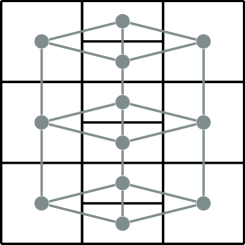
(b) The associated dual graph

Figure 1: Tilings and their dual graph

Our constructions are based on planar tilings by rectangles. A tile is an axis-parallel closed rectangle $A\subseteq\vvmathbb R^{2}$. We will encode such a tile as a triple $(p(A),\ell_{1}(A),\ell_{2}(A))$, where $p(A)\in\vvmathbb R^{2}$ denotes its bottom-left corner, $\ell_{1}(A)$ its width (length of its projection onto the $x$-axis), and $\ell_{2}(A)$ its height (length of its projection onto the $y$-axis). A tiling $\bm{T}$ is a finite collection of interior-disjoint tiles. Denote $\left\llbracket\bm{T}\right\rrbracket\mathrel{\mathop{:}}=\bigcup_{A\in\bm{T}}A$. If $R\subseteq\vvmathbb R^{2}$, we say that $\bm{T}$ is a tiling of $R$ if $\left\llbracket\bm{T}\right\rrbracket=R$. See Figure 1(a) for a tiling of the unit square.

We associate to a tiling its dual graph $G(\bm{T})$ with vertex set $\bm{T}$ and with an edge between two tiles $A,B\in\bm{T}$ whenever $A\cap B$ has Hausdorff dimension one; in other words, $A,B$ are tangent, but not only at a corner. Denote by $\mathcal{T}$ the set of all tilings of the unit square. See Figure 1(b). For the remainder of the paper, we will consider only tilings $\bm{T}$ for which $G(\bm{T})$ is connected.

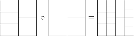
Figure 2: An example of the tiling product $S\circ T$

Definition 2.1 (Tiling product).

For $\bm{S},\bm{T}\in\mathcal{T}$, define the product $\bm{S}\circ\bm{T}\in\mathcal{T}$ as the tiling formed by replacing every tile in $\bm{S}$ by an (appropriately scaled) copy of $\bm{T}$. More precisely: For every $A\in\bm{S}$ and $B\in\bm{T}$, there is a tile $R\in\bm{S}\circ\bm{T}$ with $\ell_{i}(R)\mathrel{\mathop{:}}=\ell_{i}(A)\ell_{i}(B)$, and

$$p_{i}(R)\mathrel{\mathop{:}}=p_{i}(A)+p_{i}(B)\ell_{i}(A),$$

for each $i\in\{1,2\}$. See Figure 2.

If $\bm{T}\in\mathcal{T}$ and $n\geqslant 0$, we will use $\bm{T}^{n}\mathrel{\mathop{:}}=\bm{T}\circ\cdots\circ\bm{T}$ to denote the $n$-fold tile product of $\bm{T}$ with itself. The following observation shows that this is well-defined.

Observation 2.2.

The tiling product is associative: $(\bm{S}\circ\bm{T})\circ\bm{U}=\bm{S}\circ(\bm{T}\circ\bm{U})$ for all $S,T,U\in\mathcal{T}$. Moreover, if $\bm{I}\in\mathcal{T}$ consists of the single tile $[0,1]^{2}$, then $\bm{T}\circ\bm{I}=\bm{I}\circ\bm{T}$ for all $\bm{T}\in\mathcal{T}$.

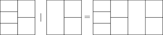
Figure 3: An example of the tiling concatenation $S\mid T$

Definition 2.3 (Tiling concatenation).

Suppose that $\bm{S}$ is a tiling of a rectangle $R$ and $\bm{T}$ is a tiling of a rectangle $R^{\prime}$ and the heights of $R$ and $R^{\prime}$ coincide. Let $R^{\prime\prime}$ denote the translation of $R^{\prime}$ for which the left edge of $R^{\prime\prime}$ coincides with the right edge of $R$, and denote by $\bm{S}\mid\bm{T}$ the induced tiling of the rectangle $R\cup R^{\prime\prime}$. See Figure 3.

Figure 4: The tiling $\bm{H}^{1}\mid\bm{H}^{2}\mid\bm{H}^{3}$

Let $\bm{H}$ denote the tiling in Figure 1(a), and define $\mathcal{H}_{n}\mathrel{\mathop{:}}=G(\bm{H}^{0}\mid\bm{H}^{1}\mid\cdots\mid\bm{H}^{n})$; see Figure 4, where we have omitted $\bm{H}^{0}$ for ease of illustration. The next theorem represents our primary goal for the remainder of this section. Note that $\bm{H}^{0}=\{\rho\}$ consists of a single tile, and that $\{(\mathcal{H}_{n},\rho)\}$ forms a Cauchy sequence in $(\mathcal{G}_{\bullet},\vvmathbb{d}_{\mathrm{loc}})$, since $(\mathcal{H}_{n},\rho)$ is naturally a rooted subgraph of $(\mathcal{H}_{n+1},\rho)$. Letting $\mathcal{H}_{\infty}$ denote its limit, we will establish the following.

Theorem 2.4.

The infinite planar graph $\mathcal{H}_{\infty}$ is transient and has uniform polynomial volume growth of degree $\log_{3}(12)$.

Uniform growth is established in Lemma 2.11 and transience in Corollary 2.17.

2.2 Volume growth

The following lemma shows that a ball of radius $r=\mathrm{diam}(\bm{H}^{n})$ in $\bm{H}^{n}$ has volume $\asymp r^{\log_{3}(12)}$. Later on, in Lemma 2.10, we will show a similar bound holds for balls of arbitrary radius $1\leqslant r\leqslant\mathrm{diam}(\bm{H}^{n})$ in $\bm{H}^{n}$.

Lemma 2.5.

For $n\geqslant 0$, we have $|\bm{H}^{n}|=12^{n}$, and $3^{n}\leqslant\mathrm{diam}(\bm{H}^{n})\leqslant 3^{n+1}$.

Proof.

The first claim is straightforward by induction. For the second claim, note that $\ell_{1}(A)=3^{-n}$ for every $A\in\bm{H}^{n}$. Moreover, there are $3^{n}$ tiles touching the left-most boundary of $[0,1]^{2}$. Therefore to connect any $A,B\in\bm{H}^{n}$ by a path in $G(\bm{H}^{n})$, we need only go from $A$ to the left-most column in at most $3^{n}$ steps, then use at most $3^{n}$ steps of the column, and finally move at most $3^{n}$ steps to $B$. ∎

The next lemma is straightforward.

Lemma 2.6.

Consider $\bm{S},\bm{T}\in\mathcal{T}$ and $G=G(\bm{S}\circ\bm{T})$. For any $X\in\bm{S}\circ\bm{T}$, it holds that $|B_{G}(X,\mathrm{diam}(G(\bm{T})))|\geqslant|\bm{T}|$.

If $\bm{T}$ is a tiling, let us partition the edge set $E(G(\bm{T}))=E_{1}(\bm{T})\cup E_{2}(\bm{T})$ into horizontal and vertical edges. For $A\in\bm{T}$ and $i\in\{1,2\}$, let $N_{\bm{T}}(A,i)$ denote the set of tiles adjacent to $A$ in $G(\bm{T})$ along the $i$th direction, meaning that the edge separating them is parallel to the $i$th axis (see Figure 5).

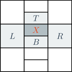
Figure 5: A tile $X\in\bm{H}$ and its neighbors are marked. Here we have $N_{\bm{H}}(X,1)=\{T,B\}$ and $N_{\bm{H}}(X,2)=\{L,R\}$.

Further denote $N_{\bm{T}}(A)\mathrel{\mathop{:}}=N_{\bm{T}}(A,1)\cup N_{\bm{T}}(A,2)$. Moreover, we define:

$$\alpha_{\bm{T}}(A,i) \mathrel{\mathop{:}}=\max\left\{\frac{\ell_{j}(A)}{\ell_{j}(B)}:B\in N_{\bm{T}}(A,i),j\in\{1,2\}\right\},\quad i\in\{1,2\}$$

$$\alpha_{\bm{T}}(A) \mathrel{\mathop{:}}=\max_{i\in\{1,2\}}\alpha_{\bm{T}}(A,i)$$

$$\alpha_{\bm{T}} \mathrel{\mathop{:}}=\max\left\{\alpha_{\bm{T}}(A):A\in\bm{T}\right\}$$

$$L_{\bm{T}} \mathrel{\mathop{:}}=\max\left\{\ell_{i}(A):A\in\bm{T},i\in\{1,2\}\right\}.$$ (2.1)

We take $\alpha_{\bm{T}}\mathrel{\mathop{:}}=1$ if $\bm{T}$ contains a single tile. It is now straightforward to check that $\alpha_{\bm{T}}$ bounds the degrees in $G(\bm{T})$.

Lemma 2.7.

For a tiling $\bm{T}$ and $A\in\bm{T}$, it holds that

$$\deg_{G(\bm{T})}(A)\leqslant 4(1+\alpha_{\bm{T}})\leqslant 8\alpha_{\bm{T}}.$$

Proof.

After accounting for the four corners of $A$, every other tile $B\in N_{\bm{T}}(A,i)$ intersects $A$ in a segment of length at least $\ell_{i}(B)\geqslant\ell_{i}(A)/\alpha_{\bm{T}}$. The second inequality follows from $\alpha_{\bm{T}}\geqslant 1$. ∎

Lemma 2.8.

Consider $\bm{S},\bm{T}\in\mathcal{T}$ and let $G=G(\bm{S}\circ\bm{T})$. Then for any $X\in\bm{S}\circ\bm{T}$, it holds that

$$|B_{G}(X,1/(\alpha^{4}_{\bm{S}}L_{\bm{T}}))|\leqslant 192\alpha^{2}_{\bm{S}}|\bm{T}|.$$ (2.2)

Proof.

For a tile $Y\in\bm{S}\circ\bm{T}$, let $\hat{Y}\in\bm{S}$ denote the unique tile for which $Y\subseteq\hat{Y}$. Let us also define

$$\tilde{N}_{\bm{S}}(\hat{X})\mathrel{\mathop{:}}=\{\hat{X}\}\cup N_{\bm{S}}(\hat{X})\cup N_{\bm{S}}\left(N_{\bm{S}}(\hat{X},1),2\right)\cup N_{\bm{S}}\left(N_{\bm{S}}(\hat{X},2),1\right),$$

which is the set of vertices of $G(\bm{S})$ that can be reached from $\hat{X}$ by following at most one edge in each direction.

We will show that

$$\left\llbracket B_{G}(X,1/(\alpha^{4}_{\bm{S}}L_{\bm{T}}))\right\rrbracket\subseteq\left\llbracket\tilde{N}_{\bm{S}}(\hat{X})\right\rrbracket.$$ (2.3)

It follows that

$$|B_{G}(X,1/(\alpha^{4}_{\bm{S}}L_{\bm{T}}))|\leqslant|\bm{T}|\cdot|\tilde{N}_{\bm{S}}(\hat{X})|\leqslant|\bm{T}|\cdot 3\left(\max_{A\in\bm{S}}\deg_{G(\bm{S})}(A)\right)^{2},$$

and then (2.2) follows from Lemma 2.7.

To establish (2.3), consider any path $\left\langle X=X_{0},X_{1},X_{2},\ldots,X_{h}\right\rangle$ in $G$ with $\hat{X}_{h}\notin\tilde{N}_{\bm{S}}(\hat{X})$. Let $k\leqslant h$ be the smallest index for which $\hat{X}_{k}\notin\tilde{N}_{\bm{S}}(\hat{X})$. Then:

$${X_{0}},{X_{1}},\ldots,{X_{k-1}}\subseteq\left\llbracket\tilde{N}_{\bm{S}}(\hat{X})\right\rrbracket$$ (2.4)

$$X_{k-1}\cap\left(\partial\left\llbracket\tilde{N}_{\bm{S}}(\hat{X})\right\rrbracket\cap(0,1)^{2}\right)\neq\emptyset.$$ (2.5)

Now (2.4) implies that

$$\ell_{i}(X_{j})\leqslant L_{\bm{T}}\ell_{i}(\hat{X}_{j})\leqslant L_{\bm{T}}\alpha^{2}_{\bm{S}}\ell_{i}(\hat{X}),\qquad j\leqslant k-1,i\in\{1,2\}.$$ (2.6)

And (2.5) shows that for some $i^{\prime}\in\{1,2\}$,

$$\sum_{j=0}^{k-1}\ell_{i^{\prime}}(X_{j})\geqslant\min\left\{\ell_{i^{\prime}}(Y):Y\in\tilde{N}_{\bm{S}}(\hat{X})\right\}\geqslant\ell_{i^{\prime}}(\hat{X})/\alpha^{2}_{\bm{S}}.$$ (2.7)

To clarify why this is true, note that

$$\hat{X}+\left[-\ell_{1}(\hat{X})/\alpha^{2}_{\bm{S}},\ell_{1}(\hat{X})/\alpha^{2}_{\bm{S}}\right]\times\left[-\ell_{2}(\hat{X})/\alpha_{\bm{S}}^{2},\ell_{2}(\hat{X})/\alpha^{2}_{\bm{S}}\right]\subseteq\left\llbracket\tilde{N}_{\bm{S}}(\hat{X})\right\rrbracket,$$

where ’$+$’ here is the Minkowski sum $R+S\mathrel{\mathop{:}}=\{r+s:r\in R,s\in S\}$. Indeed, this inclusion motivates our definition of the “$\ell_{\infty}$ neighborhood” $\tilde{N}$ above.

Combining (2.6) and (2.7) now gives

$$h\geqslant k\geqslant\frac{1}{\alpha_{\bm{S}}^{4}L_{\bm{T}}},$$

completing the proof. ∎

We can now finish the analysis of the volume growth in the graphs $\{\bm{H}^{n}:n\geqslant 0\}$.

Lemma 2.9.

For $n\geqslant 1$, it holds that $\alpha_{\bm{H}^{n}}\leqslant 2$.

Proof.

Consider $A\in\bm{H}^{n}$ and $B\in N_{\bm{H}^{n}}(A)$. First note that, as in the proof of Lemma 2.5, all the tiles in $\bm{H}^{n}$ have the same width $3^{-n}$, and so $\ell_{1}(A)=\ell_{1}(B)$. Moreover, one can easily verify that every two vertically adjacent tiles in $\bm{H}^{n}$ have the same height, and so we have $\ell_{2}(A)=\ell_{2}(B)$ when $B\in N_{\bm{H}^{n}}(A,1)$. Now we prove by an induction on $n$ that for all horizontally adjacent tiles $A,B\in\bm{H}^{n}$ we have

$$\frac{\ell_{2}(A)}{\ell_{2}(B)}\leqslant 2.$$

The base case is clear for $n=1$. For $n\geqslant 2$ Let us write $\bm{H}^{n}=\bm{H}\circ\bm{H}^{n-1}$, and let $\hat{A},\hat{B}\in\bm{H}$ be the unique tiles for which $A\subseteq\hat{A}$ and $B\subseteq\hat{B}$. If $\hat{A}=\hat{B}$, then the claim follows from the induction hypothesis. Otherwise, as $B\in N_{\bm{H}^{n}}(A,2)$, it holds that $\hat{B}\in N_{\bm{H}}(\hat{A},2)$ as well. By symmetry, the tiles touching the left and right edges of $\bm{H}^{n-1}$ have the same height, and therefore it follows that

$$\frac{\ell_{2}(A)}{\ell_{2}(B)}\leqslant\frac{\ell_{2}(\hat{A})}{\ell_{2}(\hat{B})}\leqslant 2,$$

completing the proof.

∎

Lemma 2.10.

For any $n\geqslant 0$, it holds that

$$\left|B_{G(\bm{H}^{n})}(A,r)\right|\asymp r^{\log_{3}(12)},\qquad\forall A\in\bm{H}^{n},1\leqslant r\leqslant\mathrm{diam}(G(\bm{H}^{n})).$$

Proof.

Writing $\bm{H}^{n}=\bm{H}^{n-k}\circ\bm{H}^{k}$ and employing Lemma 2.6 together with Lemma 2.5 gives

$$\left|B_{G(\bm{H}^{n})}(A,3^{k+1})\right|\geqslant|\bm{H}^{k}|=12^{k},\qquad\forall A\in\bm{H}^{n},k\in\{0,1,\ldots,n\}.$$

The desired lower bound now follows using monotonicity of $|B_{G(H^{n})}(A,r)|$ with respect to $r$.

To prove the upper bound, first note that we have $L_{\bm{H}^{k}}=3^{-k}$ (recall the definition (2.1)). Moreover, by Lemma 2.9 we have $\alpha_{\bm{H}^{n}}\leqslant 2$. Hence invoking Lemma 2.8 with $\bm{S}=\bm{H}^{n-k}$ and $\bm{T}=\bm{H}^{k}$ gives

$$\left|B_{G(\bm{H}^{n})}(A,3^{k}/16)\right|\leqslant 768\cdot 12^{k},\qquad\forall A\in\bm{H}^{n},k\in\{0,1,\ldots,n\},$$

completing the proof. ∎

Finally, this allows us to establish a uniform polynomial growth rate for $\mathcal{H}_{\infty}$.

Lemma 2.11.

It holds that

$$|B_{\mathcal{H}_{\infty}}(v,r)|\asymp r^{\log_{3}(12)}\qquad\forall v\in V(\mathcal{H}_{\infty}),r\geqslant 1.$$

Proof.

Recall first the natural identification $\bm{H}^{n}\hookrightarrow V(\mathcal{H}_{\infty})$ under which $V(\mathcal{H}_{\infty})=\bigcup_{n\geqslant 0}\bm{H}^{n}$ is a partition. Consider $v\in V(\mathcal{H}_{\infty})$ and let $n\geqslant 0$ be such that $v\in\bm{H}^{n}$. Now Lemma 2.10 in conjunction with Lemma 2.5 yields the bounds:

$$|B_{\mathcal{H}_{\infty}}(v,r)| \geqslant|B_{\mathcal{H}_{\infty}}(v,r)\cap\bm{H}^{n}|\gtrsim r^{\log_{3}(12)} r\leqslant 3^{n+3}$$

$$|B_{\mathcal{H}_{\infty}}(v,r)| \geqslant|\bm{H}^{k}|=12^{k}\gtrsim r^{\log_{3}(12)} r\in[3^{k+3},3^{k+4}),k\geqslant n$$

$$|B_{\mathcal{H}_{\infty}}(v,r)| =|B_{\mathcal{H}_{\infty}}(v,r)\cap\bm{H}^{n-1}|+|B_{\mathcal{H}_{\infty}}(v,r)\cap\bm{H}^{n}|+|B_{\mathcal{H}_{\infty}}(v,r)\cap\bm{H}^{n+1}|$$

$$\lesssim r^{\log_{3}(12)} r\leqslant 3^{n-1}$$

$$|B_{\mathcal{H}_{\infty}}(v,r)| \leqslant\sum_{j\leqslant\max(k,n+1)}|\bm{H}^{j}|\leqslant 2\cdot 12^{\max(k,n+1)}\lesssim r^{\log_{3}(12)} r\in[3^{k-1},3^{k}),k\geqslant n.$$

These four bounds together verify the desired claim. ∎

2.3 Effective resistances

Consider a weighted, undirected graph $G=(V,E,c)$ with edge conductances $c:E\to\vvmathbb R_{+}$. For $p\geqslant 1$, denote $\ell_{p}(V)\mathrel{\mathop{:}}=\{f:V\to\vvmathbb R\mid\sum_{u\in V}|f(u)|^{p}<\infty\}$, and equip $\ell_{2}(V)$ with the inner product $\langle f,g\rangle=\sum_{u\in V}f(u)g(u)$.

For $s,t\in\ell_{1}(V)$ with $\|s\|_{1}=\|t\|_{1}$, we define the effective resistance

$$\mathsf{R}_{\mathrm{eff}}^{G}(s,t)\mathrel{\mathop{:}}=\left\langle s-t,L_{G}^{\dagger}(s-t)\right\rangle,$$

where $L_{G}$ is the combinatorial Laplacian of $G$, and $L_{G}^{\dagger}$ is the Moore-Penrose pseudoinverse. Here, $L_{G}$ is the operator on $\ell_{2}(V)$ defined by

$$L_{G}f(v)=\sum_{u:\{u,v\}\in E}c(\{u,v\})\left(f(v)-f(u)\right).$$

If $G$ is unweighted, we assume it is equipped with unit conductances $c\equiv\vvmathbb{1}_{E(G)}$.

Equivalently, if we consider mappings $\theta:E\to\vvmathbb R$, and define the energy functional

$$\mathcal{E}_{G}(\theta)\mathrel{\mathop{:}}=\sum_{e\in E}c(e)^{-1}\theta(e)^{2},$$

then $\mathsf{R}_{\mathrm{eff}}^{G}(s,t)$ is the minimum energy of a flow with demands $s-t$. (See, for instance, [LP16, Ch. 2].) For two finite sets $A,B\subseteq V$ in a graph, we define

$$\mathsf{R}_{\mathrm{eff}}^{G}(A\leftrightarrow B)\mathrel{\mathop{:}}=\inf\left\{\mathsf{R}_{\mathrm{eff}}^{G}(s,t):\operatorname{supp}(s)\subseteq A,\operatorname{supp}(t)\subseteq B,s,t\in\ell_{1}(V),\|s\|_{1}=\|t\|_{1}=1\right\},$$

and we recall the following standard characterization (see, e.g., [LP16, Thm. 2.3]).

If we define additionally $c_{v}\mathrel{\mathop{:}}=\sum_{u\in V(L)}c(\{u,v\})$ for $v\in V$, then we can recall that weighted random walk $\{X_{t}\}$ on $G$ with Markovian law

$$\operatorname*{\vvmathbb{P}}\left[X_{t+1}=v\mid X_{t}=u\right]=\frac{c(\{u,v\})}{c_{u}},\qquad u,v\in V.$$

Theorem 2.12 (Transience criterion).

A weighted graph $G=(V,E,c)$ is transient if and only if there is a vertex $v\in V$ and an increasing sequence $V_{1}\subseteq\cdots\subseteq V_{n}\subseteq V_{n+1}\subseteq\cdots$ of finite subsets of vertices satisfying $\bigcup_{n\geqslant 1}V_{n}=V$ and

$$\sup_{n\geqslant 1}\mathsf{R}_{\mathrm{eff}}^{G}\left(\{v\}\leftrightarrow V\setminus V_{n}\right)<\infty.$$

For a tiling $\bm{T}$ of a closed rectangle $R$, let $\mathscr{L}(\bm{T})$ and $\mathscr{R}(\bm{T})$ denote the sets of tiles that intersect the left and right edges of $R$, respectively. We define

$$\rho(\bm{T})\mathrel{\mathop{:}}=\mathsf{R}_{\mathrm{eff}}^{G(\bm{T})}\left(\vvmathbb{1}_{\mathscr{L}(\bm{T})}/|\mathscr{L}(\bm{T})|,\vvmathbb{1}_{\mathscr{R}(\bm{T})}/|\mathscr{R}(\bm{T})|\right),$$

Observation 2.13.

For any $\bm{S},\bm{T}\in\mathcal{T}$, we have $|\mathscr{L}(\bm{S}\circ\bm{T})|=|\mathscr{L}(\bm{S})|\cdot|\mathscr{L}(\bm{T})|$ and $|\mathscr{R}(\bm{S}\circ\bm{T})|=|\mathscr{R}(\bm{S})|\cdot|\mathscr{R}(\bm{T})|$. In particular, $|\mathscr{L}(\bm{H}^{n})|=|\mathscr{R}(\bm{H}^{n})|=3^{n}$.

Lemma 2.14.

Suppose that $\bm{S},\bm{T}$ are tilings satisfying the conditions of Definition 2.3. Suppose furthermore that all rectangles in $\mathscr{R}(\bm{S})$ have the same height, and the same is true for $\mathscr{L}(\bm{T})$. Then we have

$$\rho(\bm{S}\mid\bm{T})\leqslant\rho(\bm{S})+\rho(\bm{T})+\frac{1}{\max(|\mathscr{R}(\bm{S})|,|\mathscr{L}(\bm{T})|)}\,.$$

Proof.

By the triangle inequality for effective resistances, it suffices to prove that

$$\mathsf{R}_{\mathrm{eff}}^{G}\left(\vvmathbb{1}_{\mathscr{R}(\bm{S})}/|\mathscr{R}(\bm{S})|,\vvmathbb{1}_{\mathscr{L}(\bm{T})}/|\mathscr{L}(\bm{T})|\right)\leqslant\frac{1}{\max(|\mathscr{R}(\bm{S})|,|\mathscr{L}(\bm{T})|)}\,,$$

where $G=G(\bm{S}\mid\bm{T})$. We construct a flow from $\mathscr{R}(\bm{S})$ to $\mathscr{L}(\bm{T})$ as follows: If $A\in\mathscr{R}(\bm{S}),B\in\mathscr{L}(\bm{T})$ and $\{A,B\}\in E(G)$, then the flow value on $\{A,B\}$ is

$$F_{AB}\mathrel{\mathop{:}}=\frac{\mathrm{len}(A\cap B)}{\ell_{2}(A)}\frac{1}{|\mathscr{R}(\bm{S})|}.$$

Denoting $m\mathrel{\mathop{:}}=\max(|\mathscr{R}(\bm{S})|,|\mathscr{L}(\bm{T})|)$, we clearly have $F_{AB}\leqslant 1/m$. Moreover,

$$\sum_{A\in\mathscr{R}(\bm{S})}\sum_{\begin{subarray}{c}B\in\mathscr{L}(\bm{T}):\\ \{A,B\}\in E(G)\end{subarray}}F_{AB}=1,$$

hence

$$\sum_{A\in\mathscr{R}(\bm{S})}\sum_{\begin{subarray}{c}B\in\mathscr{L}(\bm{T}):\\ \{A,B\}\in E(G)\end{subarray}}F_{AB}^{2}\leqslant 1/m,$$

completing the proof. ∎

Say that a tiling $\bm{T}$ is non-degenerate if $\mathcal{L}(\bm{T})\cap\mathcal{R}(\bm{T})=\emptyset$, i.e., if no tile $A\in\bm{T}$ touches both the left and right edges of $\left\llbracket\bm{T}\right\rrbracket$. Let $\Delta_{\bm{T}}\mathrel{\mathop{:}}=\max_{A\in\bm{T}}\deg_{G(\bm{T})}(A)$. If $\bm{S}$ and $\bm{T}$ are non-degenerate, we have the simple inequalities $\rho(\bm{T})\geqslant 1/(\Delta_{\bm{T}}\cdot|\mathscr{L}(\bm{T})|)$ and $\rho(\bm{T})\geqslant 1/(\Delta_{\bm{T}}\cdot|\mathscr{R}(\bm{T})|)$. Together with Lemma 2.7, this yields a fact that we will employ later.

Corollary 2.15.

For any two non-degenerate tilings $\bm{S},\bm{T}$ satisfying the assumptions of Lemma 2.14, it holds that

$$\rho(\bm{S}\mid\bm{T}) \leqslant\rho(\bm{S})+\rho(\bm{T})+8\min(\alpha_{S}\rho(\bm{S}),\alpha_{T}\rho(\bm{T}))$$

$$\lesssim_{\alpha_{S},\alpha_{T}}\rho(\bm{S})+\rho(\bm{T}).$$

Lemma 2.16.

For every $n\geqslant 1$, it holds that

$$\rho(\bm{H}^{n})\lesssim(5/6)^{n}.$$

Proof.

Fix $n\geqslant 2$. Recalling Figure 1(b), let us consider $\bm{H}^{n}$ as consisting of three (identical) tilings stacked vertically, and where each of these three tilings is written as $\bm{H}^{n-1}\mid\bm{S}\mid\bm{H}^{n-1}$ where $\bm{S}$ consists of two copies of $\bm{H}^{n-1}$ stacked vertically. Applying Lemma 2.14 to $\bm{H}^{n-1}\mid\bm{S}\mid\bm{H}^{n-1}$ gives

$$\rho(\bm{H}^{n}) \leqslant(1/3)^{2}\cdot 3\left(2\rho(\bm{H}^{n-1})+\rho(\bm{S})+\frac{1}{\max(|\mathscr{R}(\bm{H}^{n-1})|,|\mathscr{L}(\bm{S})|)}+\frac{1}{\max(|\mathscr{L}(\bm{H}^{n-1})|,|\mathscr{R}(\bm{S})|)}\right)$$

$$\leqslant(1/3)^{2}\cdot 3\left(2\rho(\bm{H}^{n-1})+(1/2)^{2}\cdot 2\rho(\bm{H}^{n-1})+\frac{2}{2\cdot 3^{n-1}}\right)$$

$$=(5/6)\rho(\bm{H}^{n-1})+3^{-n},$$

where in the second inequality we have employed Observation 2.13. This yields the desired result by induction on $n$. ∎

Corollary 2.17.

The graphs $\mathcal{H}_{n}=G(\bm{H}^{0}\mid\bm{H}^{1}\mid\cdots\mid\bm{H}^{n})$ satisfy

$$\sup_{n\geqslant 1}\rho(\mathcal{H}_{n})<\infty.$$ (2.8)

Hence $\mathcal{H}_{\infty}$ is transient.

Proof.

Employing Lemma 2.14, Observation 2.13, and Lemma 2.16 together yields

$$\rho(\mathcal{H}_{n})\lesssim\sum_{j=1}^{n}\left[(5/6)^{j}+3^{-j}\right],$$

verifying (2.8). Now Theorem 2.12 yields the transience of $\mathcal{H}_{\infty}$. ∎

3 Generalizations and unimodular constructions

Consider a sequence $\gamma=\left\langle\gamma_{1},\ldots,\gamma_{b}\right\rangle$ with $\gamma_{i}\in\vvmathbb N$. Define a tiling $\bm{T}_{\gamma}\in\mathcal{T}$ as follows: The unit square is partitioned into $b$ columns of width $1/b$, and for $i\in\{1,2,\ldots,b\}$, the $i$th column has $\gamma_{i}$ rectangles of height $1/\gamma_{i}$. For instance, the tiling $\bm{H}$ from Figure 1(a) can be written $\bm{H}=\bm{T}_{\langle 3,6,3\rangle}$.

We will assume throughout this section that $\min(\gamma)=b$ and $\gamma_{1}=\gamma_{b}$. Let us use the notation $|\gamma|\mathrel{\mathop{:}}=\gamma_{1}+\cdots+\gamma_{b}$. The proof of the next lemma follows just as for Lemma 2.5 using $\min(\gamma)=b$ so that there is a column in $\bm{T}_{\gamma}^{n}$ of height $b^{n}$.

Lemma 3.1.

For $n\geqslant 0$, it holds that $|\bm{T}_{\gamma}^{n}|=|\gamma|^{n}$, and $b^{n}\leqslant\mathrm{diam}(\bm{T}_{\gamma}^{n})\leqslant 3b^{n}$.

Clearly we have $\alpha_{\bm{T}_{\gamma}}\leqslant|\gamma|/b$. The following lemma can be shown using a similar argument to that of Lemma 2.9. Note that the only symmetry required in the proof of Lemma 2.9 is that the first and last column of $\bm{T}_{\gamma}$ have the same geometry, and this is true since $\gamma_{1}=\gamma_{b}$.

Lemma 3.2.

For any $n\geqslant 1$, it holds that $\alpha_{\bm{T}_{\gamma}^{n}}\leqslant\alpha_{\bm{T}_{\gamma}}\leqslant|\gamma|/b$.

The next lemma also follows from Lemma 3.1 and the same reasoning used in the proof of Lemma 2.10. The dependence of the implicit constant on $|\gamma|/b$ comes from Lemma 3.2.

Lemma 3.3.

For any $n\geqslant 0$, it holds that

$$\left|B_{G}(A,r)\right|\asymp_{|\gamma|/b}r^{\log_{b}(|\gamma|)}\qquad\forall A\in\bm{T}_{\gamma}^{n},\ 1\leqslant r\leqslant\mathrm{diam}(G(\bm{T}_{\gamma}^{n})).$$

3.1 Degrees of growth

Consider $b,k\in\vvmathbb N$ with $k\geqslant b\geqslant 4$, and define the sequence

$$\gamma^{(b,k)}\mathrel{\mathop{:}}=\left\langle b,\underbrace{\left\lceil\frac{k-3}{b-3}\right\rceil b,\ldots,\left\lceil\frac{k-3}{b-3}\right\rceil b}_{(k-3)\bmod(b-3)\textrm{ copies}},b,\underbrace{\left\lfloor\frac{k-3}{b-3}\right\rfloor b,\ldots,\left\lfloor\frac{k-3}{b-3}\right\rfloor b}_{(b-3)-[(k-3)\bmod(b-3)]\textrm{ copies}},b\right\rangle.$$

Denote $\bm{T}_{(b,k)}\mathrel{\mathop{:}}=\bm{T}_{\gamma^{(b,k)}}$ and note that $|\gamma^{(b,k)}|=bk$. Define $\mathsf{d}_{g}(b,k)\mathrel{\mathop{:}}=\log_{b}(bk)$, and $\Gamma_{b,k}\mathrel{\mathop{:}}=\sum_{i=1}^{b}1/\gamma_{i}^{(b,k)}$.

Observation 3.4.

The following facts hold for $k\geqslant b\geqslant 4$ and $n\geqslant 0$:

1. There are $b^{n}$ tiles in the left- and right-most columns of $\bm{T}^{n}_{(b,k)}$.

2. If a pair of consecutive columns in $\bm{T}^{n}_{(b,k)}$ have heights $h$ and $h^{\prime}$, then $\min(h,h^{\prime})$ divides $\max(h,h^{\prime})$.

Now observe that Lemma 3.3 yields the following.

Corollary 3.5.

The family of graphs $\mathcal{F}=\big{\{}G\big{(}\bm{T}_{(b,k)}^{n}\big{)}:n\geqslant 0\big{\}}$ has uniform polynomial growth of degree $\mathsf{d}_{g}(b,k)$ in the sense that

$$|B_{G}(x,r)|\asymp_{k}r^{\mathsf{d}_{g}(b,k)},\qquad\forall G\in\mathcal{F},x\in V(G),1\leqslant r\leqslant\mathrm{diam}(G)\,.$$

For any rational $p/q\geqslant 2$, one can achieve $\mathsf{d}_{g}(b,k)=p/q$ by taking $b=4^{q}$ and $k=4^{p-q}$.

Remark 3.6 (Arbitrary real degrees $d>2$).

We note that by considering more general products of tilings, one can obtain planar graphs of uniform polynomial growth of any real degree $d>2$ for which the main results of this paper still hold. Instead of working with the family of powers $\{\bm{T}_{\gamma}^{n}\}$ for a fixed tiling $\bm{T}_{\gamma}$, one defines an infinite sequence $\langle\gamma^{(1)},\gamma^{(2)},\ldots\rangle$, and examines the family of graphs $\bm{T}_{\gamma^{(n)}}\circ\cdots\circ\bm{T}_{\gamma^{(1)}}$.

More concretely, fix some real $d>2$, and let us consider a sequence $\{h_{n}:n\geqslant 1\}$ of nonnegative integers. Also define $\gamma^{(n)}\mathrel{\mathop{:}}=\gamma^{(4,4+h_{n})}$ and $\bm{T}^{(n)}\mathrel{\mathop{:}}=\bm{T}_{\gamma^{(n)}}\circ\cdots\circ\bm{T}_{\gamma^{(1)}}$. Then $|\bm{T}^{(n)}|=4^{n}\prod_{j=1}^{n}(4+h_{j})$, and $\mathrm{diam}(\bm{T}^{(n)})\asymp 4^{n}$. By a similar argument as in Lemma 2.10 based on the recursive structure, it holds that for $i\in\{1,2,\ldots,n\}$, balls of radius $\asymp 4^{i}$ in $\bm{T}^{(n)}$ have volume $\asymp_{K}4^{i}\prod_{j=1}^{i}(4+h_{j})$, where $K\mathrel{\mathop{:}}=\max\{h_{n}:n\geqslant 1\}$. Given our choice of $\{h_{1},\ldots,h_{n-1}\}$, we choose $h_{n}\geqslant 0$ as large as possible subject to

$$\sum_{j=1}^{n}\log_{4}(1+h_{j}/4)\leqslant(d-2)n.$$

It is straightforward to argue that $K\lesssim_{d}1$, and

$$\left|\sum_{j=1}^{n}\log_{4}(1+h_{j}/4)-(d-2)n\right|\lesssim_{d}1,$$

implying that $4^{n}\prod_{j=1}^{n}(4+h_{j})\asymp_{d}4^{dn}$ for every $n\geqslant 1$. It follows that the graphs $\{\bm{T}^{(n)}:n\geqslant 1\}$ have uniform polynomial growth of degree $d$.

Let us now return to the graphs $\bm{T}^{n}_{(b,k)}$ and analyze the effective resistance across them.

Lemma 3.7.

For every $n\geqslant 1$, it holds that

$$\Gamma^{n}_{b,k}\lesssim_{k}\rho\left(\bm{T}^{n}_{(b,k)}\right)\lesssim\Gamma^{n}_{b,k}\,.$$

Proof.

Fix $n\geqslant 2$ and write $\bm{T}^{n}_{(b,k)}=\bm{T}_{(b,k)}\circ\bm{T}^{n-1}_{(b,k)}$ as $\bm{A}_{1}\mid\bm{A}_{2}\mid\cdots\mid\bm{A}_{b}$ where, for $1\leqslant i\leqslant b$, each $\bm{A}_{i}$ is a vertical stack of $\gamma_{i}^{(b,k)}$ copies of $\bm{T}^{n-1}_{(b,k)}$. Since $\rho(\bm{A}_{i})=\rho(\bm{T}_{(b,k)}^{n-1})/\gamma_{i}^{(b,k)}$ by the parallel law for effective resistances, applying Lemma 2.14 to $\bm{A}_{1}\mid\bm{A}_{2}\mid\cdots\mid\bm{A}_{b}$ gives

$$\rho\left(\bm{T}^{n}_{(b,k)}\right) \leqslant\sum_{i-1}^{b}\rho(\bm{T}_{(b,k)}^{n-1})/\gamma_{i}^{(b,k)}+\sum_{i=1}^{b-1}\frac{1}{\min\left(\mathscr{R}(\bm{A}_{i}),\mathscr{L}(\bm{A}_{i+1})\right)}\leqslant\rho(\bm{T}^{n-1}_{(b,k)})\Gamma_{b,k}+b^{1-n},$$

where in the second inequality we have employed $\min\left(\mathscr{R}(\bm{A}_{i}),\mathscr{L}(\bm{A}_{i+1})\right)\geqslant b^{n}$ which follows from Observation 3.4(a). Finally, observe that $\Gamma_{b,k}\geqslant 1/\gamma_{1}^{(b,k)}+1/\gamma_{b}^{(b,k)}=2/b$, and therefore the desired upper bound follows by induction.

For the lower bound, note that since the degrees in $\bm{T}^{n}_{(b,k)}$ are bounded by $k$, the Nash-Williams inequality (see, e.g., [LP16, §5]) gives

$$\rho(\bm{T}^{n}_{(b,k)})\gtrsim_{k}\sum_{i=2}^{b^{n}-1}\frac{1}{|K_{i}|}\gtrsim\sum_{i=1}^{b^{n}}\frac{1}{|K_{i}|}=\Gamma_{b,k}^{n},$$ (3.1)

where $K_{i}$ is the $i$th column of rectangles in $\bm{T}^{n}_{(b,k)}$, and the last equality follows by a simple induction. ∎

The next result establishes Theorem 1.1.

Theorem 3.8.

For every $k>b$, the graphs $\mathcal{T}_{n}^{(b,k)}\mathrel{\mathop{:}}=G\left(\bm{T}^{0}_{(b,k)}\mid\bm{T}^{1}_{(b,k)}\mid\cdots\mid\bm{T}^{n}_{(b,k)}\right)$ satisfy

$$\sup_{n\geqslant 1}\rho\left(\mathcal{T}_{n}^{(b,k)}\right)<\infty.$$ (3.2)

Hence the limit graph $\mathcal{T}_{\infty}^{(b,k)}$ is transient. Moreover, $\mathcal{T}_{\infty}^{(b,k)}$ has uniform polynomial growth of degree $\mathsf{d}_{g}(b,k)$.

Proof.

Employing Lemma 2.14, Observation 3.4(a), and Lemma 3.7 together yields

$$\rho\left(\mathcal{T}_{n}^{(b,k)}\right)\lesssim\sum_{j=1}^{n}\left(\Gamma_{b,k}^{j}+b^{-j}\right).$$

For $k>b$, we have $\max(\gamma^{(b,k)})>b$ and $\min(\gamma^{(b,k)})=b$, hence $\Gamma_{b,k}<1$, verifying (3.2). Now Theorem 2.12 yields transience of $\mathcal{T}_{\infty}^{(b,k)}$.

Uniform polynomial growth of degree $\mathsf{d}_{g}(b,k)$ follows from Corollary 3.5 as in the proof of Lemma 2.11. ∎

3.2 The distributional limit

Fix $k\geqslant b\geqslant 4$ and take $G_{n}\mathrel{\mathop{:}}=G(\bm{T}_{(b,k)}^{n})$. Since the degrees in $\{G_{n}\}$ are uniformly bounded, the sequence has a subsequential distributional limit, and in all arguments that follow, we could consider any such limit. But let us now argue that if $\mu_{n}$ is the law of $(G_{n},\rho_{n})$ with $\rho_{n}\in V(G_{n})$ chosen according to the stationary measure, then the measures $\{\mu_{n}:n\geqslant 0\}$ have a distributional limit.

Lemma 3.9.

For any $k\geqslant b\geqslant 4$, there is a reversible random graph $(G_{b,k},\rho)$ such that $\{(G_{n},\rho_{n})\}\Rightarrow(G_{b,k},\rho)$. Moreover, almost surely $G_{b,k}$ has uniform polynomial volume growth of degree $\mathsf{d}_{g}(b,k)$.

Proof.

It suffices to prove that $\{(G_{n},\rho_{n})\}$ has a limit $(G_{b,k},\rho)$. Reversibility of the limit then follows automatically (as noted in Section 1.1.1), and the degree of growth is an immediate consequence of Corollary 3.5. It will be slightly easier to show that the sequence $\{(G_{n},\hat{\rho}_{n})\}$ has a distributional limit, with $\hat{\rho}_{n}\in V(G_{n})$ chosen uniformly at random. As noted in Section 1.1.1, the claim then follows from [BC12, Prop. 2.5] (the correspondence between unimodular and reversible random graphs under degree-biasing).

Let $\mu_{n,r}$ be the law of $B_{G_{n}}(\hat{\rho}_{n},r)$. It suffices to show that the measures $\{\mu_{n,r}:n\geqslant 0\}$ converge for every fixed $r\geqslant 1$, and then a standard application of Kolmogorov’s extension theorem proves the existence of a limit.

For a tiling $\bm{T}$ of a rectangle $R$, let $\partial\bm{T}$ denote the set of tiles that intersect some side of $R$. Define the neighborhood $N_{r}(\partial\bm{T}_{(b,k)}^{n})\mathrel{\mathop{:}}=\{v\in\bm{T}^{n}_{(b,k)}:d_{G_{n}}(v,\partial\bm{T}_{(b,k)}^{n})\leqslant r\}$ and abbreviate $\mathsf{d}=\mathsf{d}_{g}(b,k)$. Then $|\partial\bm{T}^{n}_{(b,k)}|\leqslant 4b^{n}$, so Corollary 3.5 gives

$$\left|N_{r}(\partial\bm{T}^{n}_{(b,k)})\right|\lesssim_{k}b^{n}r^{\mathsf{d}}\,.$$

Since $|\bm{T}^{n}_{(b,k)}|=(bk)^{n}$, it follows that

$$1-\operatorname*{\vvmathbb{P}}\left[\mathcal{E}_{r,n}\right]\lesssim_{k}k^{-n}r^{\mathsf{d}},$$

where $\mathcal{E}_{r,n}$ is the event $\{B_{G_{n}}(\hat{\rho}_{n},r)\cap\partial\bm{T}^{n}_{(b,k)}=\emptyset\}$.

Now write $\bm{T}^{n}_{(b,k)}=\bm{T}_{(b,k)}\circ\bm{T}^{n-1}_{(b,k)}$, and note that $\hat{\rho}_{n}$ falls into one of the $|\gamma^{(b,k)}|=bk$ copies of $G_{n-1}$ and is, moreover, uniformly distributed in that copy. Therefore we can naturally couple $(G_{n},\hat{\rho}_{n})$ and $(G_{n-1},\hat{\rho}_{n-1})$ by identifying $\hat{\rho}_{n}$ with $\hat{\rho}_{n-1}$. Moreover, conditioned on the event $\mathcal{E}_{r,n-1}$, we can similarly couple $B_{G_{n}}(\hat{\rho}_{n},r)$ and $B_{G_{n-1}}(\hat{\rho}_{n-1},r)$.

It follows that, for every $r\geqslant 1$,

$$d_{TV}\left(\mu_{n-1,r},\mu_{n,r}\right)\leqslant 1-\operatorname*{\vvmathbb{P}}[\mathcal{E}_{r,n-1}]\lesssim_{k}k^{-n}r^{\mathsf{d}}\,.$$

As the latter sequence is summable, it follows that $\{\mu_{n,r}\}$ converges for every fixed $r\geqslant 1$, completing the proof. ∎

3.3 Speed of the random walk

Let $\{X_{t}\}$ denote the random walk on $G_{b,k}$ with $X_{0}=\rho$. Our first goal will be to prove a lower bound on the speed of the walk. Define:

$$\mathsf{d}_{w}(b,k) \mathrel{\mathop{:}}=\mathsf{d}_{g}(b,k)+\log_{b}(\Gamma_{b,k}).$$

We will show that $\mathsf{d}_{w}(b,k)$ is related to the speed exponent for the random walk.

Theorem 3.10.

Consider any $k\geqslant b\geqslant 4$. It holds that for all $T\geqslant 1$,

$$\operatorname*{\vvmathbb{E}}\left[d_{G_{b,k}}\!\left(X_{T},X_{0}\right)\mid X_{0}=\rho\right]\gtrsim_{k}T^{1/\mathsf{d}_{w}(b,k)}.$$ (3.3)

Before proving the theorem, let us observe that it yields Theorem 1.3. Fix $k\geqslant b\geqslant 4$. Observe that for any positive integer $p\geqslant 1$, we have $\mathsf{d}_{g}(b^{p},k^{p})=\mathsf{d}_{g}(b,k)$. On the other hand,

$$\mathsf{d}_{g}(b^{p},k^{p})-\mathsf{d}_{w}(b^{p},k^{p}) =-\log_{b^{p}}(\Gamma_{b^{p},k^{p}})$$

$$\geqslant-\log_{b^{p}}\left(3b^{-p}+(b/k)^{p}\right)-o_{p}(1)$$

$$\geqslant\min\left(1,\log_{b}(k)-1\right)-o_{p}(1)$$

$$\geqslant\min\left(1,\mathsf{d}_{g}(b^{p},k^{p})-2\right)-o_{p}(1)\,.$$ (3.4)

So for every $\varepsilon>0$, there is some $p=p(\varepsilon)$ such that

$$\mathsf{d}_{w}(b^{p},k^{p})\leqslant\max\left(2,\mathsf{d}_{g}(b^{p},k^{p})-1\right)+\varepsilon\,,$$

and moreover $G_{b^{p},k^{p}}$ almost surely has uniform polynomial growth of degree $\mathsf{d}_{g}(b,k)$. Combining this with the construction of Corollary 3.5 for all rational $d\geqslant 2$ yields Theorem 1.3.

3.3.1 The linearized graphs

Fix integers $k\geqslant b\geqslant 4$ and $n\geqslant 1$, and let us consider now the (weighted) graph $L=L_{(b,k)}^{n}$ derived from $G=G(\bm{T}_{(b,k)}^{n})$ by identifying every column of rectangles into a single vertex. Thus $|V(L)|=b^{n}$.

We connect two vertices $u,v\in V(L)$ if their corresponding columns $\mathcal{C}_{u}$ and $\mathcal{C}_{v}$ in $G$ are adjacent, and we define the conductances $c_{uv}\mathrel{\mathop{:}}=|E_{G}(\mathcal{C}_{u},\mathcal{C}_{v})|$, where $E_{G}(S,T)$ denotes the number of edges between two subsets $S,T\subseteq V(G)$. Define additionally $c_{uu}\mathrel{\mathop{:}}=2|\mathcal{C}_{u}|$ and

$$c_{u} \mathrel{\mathop{:}}=c_{uu}+\sum_{v:\{u,v\}\in E(L)}c(\{u,v\})\,.$$

Let us order the vertices of $L$ from left to right as $V(L)=\{\ell_{1},\ldots,\ell_{b^{n}}\}$. The series law for effective resistances gives the following.

Observation 3.11.

For $1\leqslant i\leqslant t\leqslant j\leqslant b^{n}$, we have

$$\mathsf{R}_{\mathrm{eff}}^{L}(\ell_{i}\leftrightarrow\ell_{j})=\mathsf{R}_{\mathrm{eff}}^{L}(\ell_{i}\leftrightarrow\ell_{t})+\mathsf{R}_{\mathrm{eff}}^{L}(\ell_{t}\leftrightarrow\ell_{j})$$

We will use this to bound the resistance between any pair of columns.

Lemma 3.12.

If $1\leqslant s<t\leqslant b^{n}$, then

$$\mathsf{R}_{\mathrm{eff}}^{L}(\ell_{s}\leftrightarrow\ell_{t})\cdot\left(c_{\ell_{s}}+c_{\ell_{s+1}}+\cdots+c_{\ell_{t}}\right)\asymp_{k}(\Gamma_{b,k}\cdot bk)^{\log_{b}(t-s)}\,.$$ (3.5)

Proof.

Let us first establish the upper bound. Denote $h\mathrel{\mathop{:}}=\lceil\log_{b}(t-s)\rceil$, $\bm{T}\mathrel{\mathop{:}}=\bm{T}_{(b,k)}$, and $\Gamma\mathrel{\mathop{:}}=\Gamma_{b,k}$. Write $\bm{T}^{n}=\bm{T}^{n-h}\circ\bm{T}^{h}$ and along this decomposition, partition $\bm{T}^{n}$ into $b^{n-h}$ sets of tiles $\mathcal{D}_{1},\ldots,\mathcal{D}_{b^{n-h}}$, where each $\mathcal{D}_{i}$ is formed from adjacent columns

$$\mathcal{D}_{i}\mathrel{\mathop{:}}=\mathcal{C}_{(i-1)\cdot b^{h}+1}\cup\cdots\cup\mathcal{C}_{i\cdot b^{h}}\,.$$ (3.6)

Suppose that, for $1\leqslant i\leqslant b^{n-h}$, the tiling $\bm{T}^{n-h}$ has $\beta_{i}$ tiles in its $i$th column. Then $\mathcal{D}_{i}$ consists of $\beta_{i}$ copies of $\bm{T}^{h}$ stacked atop each other.

Thus we have $|\mathcal{D}_{i}|=\beta_{i}|\bm{T}^{h}|$, and furthermore $\rho(\mathcal{D}_{i})\leqslant\rho(\bm{T}^{h})/\beta_{i}$, hence

$$\rho(\mathcal{D}_{i})\cdot|\mathcal{D}_{i}|\leqslant\rho(\bm{T}^{h})\cdot|\bm{T}^{h}|\lesssim\Gamma^{h}\cdot(bk)^{h},$$ (3.7)

where the last inequality uses Lemma 3.7.

Let $1\leqslant i\leqslant j\leqslant b^{n-h}$ be such that $\mathcal{C}_{s}\subseteq\mathcal{D}_{i}$ and $\mathcal{C}_{t}\subseteq\mathcal{D}_{j}$. Since $t\leqslant s+b^{h}$, and each set $\mathcal{D}_{i}$ consists of $b^{h}$ consecutive columns, it must be that $j\leqslant i+1$. If $i=j$, then $|\mathcal{C}_{s}|+\cdots+|\mathcal{C}_{t}|\leqslant|\mathcal{D}_{i}|$, and Observation 3.11 gives

$$\mathsf{R}_{\mathrm{eff}}^{L}(\ell_{s}\leftrightarrow\ell_{t})\leqslant\rho(\mathcal{D}_{i}),$$

thus (3.7) yields (3.5), as desired.

Suppose, instead, that $j=i+1$. From Lemma 3.2, we have $\alpha_{\bm{T}^{n-h}}\leqslant|\gamma|/b\leqslant k$. Therefore $1/k\leqslant\beta_{i+1}/\beta_{i}\leqslant k$. Since the degrees in $G(\bm{T}^{n}_{(b,k)})$ are bounded by $k$, this yields the following claim, which we will also employ later.

Claim 3.13.

For any $\ell_{i}\in V(L)$, we have

$$c_{\ell_{i}}\asymp_{k}|\mathcal{C}_{i}|,$$ (3.8)

and for any $D>0$ and columns $\mathcal{C}_{a}\in\mathcal{D}_{i}$ and $\mathcal{C}_{b}\in\mathcal{D}_{j}$ with $|i-j|\leqslant D$, it holds that

$$c_{\ell_{a}}\asymp_{k}|\mathcal{C}_{a}|\asymp_{k,D}|\mathcal{C}_{b}|\asymp_{k}c_{\ell_{b}}.$$ (3.9)

Thus using Corollary 2.15 (and noting that each $\mathcal{D}_{i}$ is non-degenerate) along with (3.7) gives

$$\rho(\mathcal{D}_{i}\cup\mathcal{D}_{i+1})=\rho(\mathcal{D}_{i}\mid\mathcal{D}_{i+1})\lesssim_{k}\rho(\mathcal{D}_{i})+\rho(\mathcal{D}_{i+1})\lesssim_{k}\rho(\bm{T}^{h})/\beta_{i}.$$

Since it also holds that $|\mathcal{D}_{i}|+|\mathcal{D}_{i+1}|=(\beta_{i}+\beta_{i+1})|\bm{T}^{h}|\leqslant 2k\beta_{i}|\bm{T}^{h}|$, Observation 3.11 gives

$$\mathsf{R}_{\mathrm{eff}}^{L}(\ell_{s}\leftrightarrow\ell_{t})\cdot\left(|\mathcal{C}_{s}|+\cdots+|\mathcal{C}_{t}|\right)\leqslant\rho(\mathcal{D}_{i}\cup\mathcal{D}_{i+1})|\mathcal{D}_{i}\cup\mathcal{D}_{i+1}|\lesssim_{k}\rho(\bm{T}^{h})|\bm{T}^{h}|,$$

and again (3.7) establishes (3.5). Now (3.8) completes the proof of the upper bound.

For the lower bound, define $h^{\prime}\mathrel{\mathop{:}}=\lfloor\log_{b}(t-s)\rfloor-1$ and decompose $\bm{T}^{n}=\bm{T}^{n-h^{\prime}}\circ\bm{T}^{h^{\prime}}$. Partition $\bm{T}^{n}$ similarly into $b^{n-h^{\prime}}$ sets of tiles $\mathcal{D}_{1},\ldots,\mathcal{D}_{b^{n-h^{\prime}}}$. Suppose that $\mathcal{C}_{s}\subseteq\mathcal{D}_{i}$ and $\mathcal{C}_{t}\subseteq\mathcal{D}_{j}$, and note that the width of each $\mathcal{D}_{i}$ is $b^{h^{\prime}}$ and $b^{h^{\prime}+2}\geqslant t-s\geqslant b^{h^{\prime}+1}$, hence $j>i+1$. Therefore using again Observation 3.11 and the Nash-Williams inequality, we have

$$\mathsf{R}_{\mathrm{eff}}^{L}(\ell_{s}\leftrightarrow\ell_{t})\geqslant\sum_{j=s+1}^{t-1}\frac{1}{c_{\ell_{j}}}\stackrel{{\scriptstyle\eqref{eq:Lmass1}}}{{\gtrsim_{k}}}\sum_{j=s+1}^{t-1}\frac{1}{|\mathcal{C}_{j}|}\geqslant\sum_{j=(i-1)b^{h}+1}^{ib^{h}}\frac{1}{|\mathcal{C}_{j}|}=\frac{1}{\beta_{i+1}}\Gamma_{b,k}^{n},$$

where the final inequality uses (3.1). Note also that

$$|\mathcal{C}_{s}|+\cdots+|\mathcal{C}_{t}|\geqslant|\mathcal{D}_{i+1}|=\beta_{i+1}|\bm{T}^{h^{\prime}}|=\beta_{i+1}(bk)^{h^{\prime}}.$$

An application of (3.8) completes the proof of the lower bound. ∎

3.3.2 Rate of escape in $L$

Consider again the linearized graph $L=L^{n}_{(b,k)}$ with conductances $c:E(L)\to\vvmathbb R_{+}$ defined in Section 3.3.1, and let $\{Y_{t}\}$ be the random walk on $L$ defined by

$$\operatorname*{\vvmathbb{P}}[Y_{t+1}=v\mid Y_{t}=u]=\frac{c_{uv}}{c_{u}},\quad\{u,v\}\in E(L)\textrm{ or }u=v.$$ (3.10)

Let $\pi_{L}$ be the stationary measure of $\{Y_{t}\}$.

For a parameter $1\leqslant h\leqslant n$, consider the decomposition $\bm{T}^{n}=\bm{T}^{n-h}\circ\bm{T}^{h}$, and let $V_{1},V_{2},\ldots,V_{b^{n-h}}$ be a partition of $V(L)$ into continguous subsets with $|V_{1}|=|V_{2}|=\cdots=|V_{b}^{n-h}|=b^{h}$.

Let $\{Z_{i}:i\in\{1,2,\ldots,b^{n-h}\}\}$ be a collection of independent random variables with

$$\operatorname*{\vvmathbb{P}}[Z_{i}=v]=\frac{\pi_{L}(v)}{\pi_{L}(V_{i})},\quad v\in V_{i}.$$

Define the random time $\tau(h)$ as follows: Given $Y_{0}\in V_{j}$, let $\tau(h)$ be the first time $\tau\geqslant 1$ at which

$$Y_{\tau}\in\{Z_{j-2},Z_{j+2}\}\qquad 3\leqslant j\leqslant b^{n-h}-2$$

$$Y_{\tau}=Z_{j+2}\qquad j\in\{1,2\}$$

$$Y_{\tau}=Z_{j-2}\qquad j\in\{b^{n-h}-1,b^{n-h}\}.$$

The next lemma shows that the law of the walk stopped at time $\tau(h)$ is within a constant factor of the stationary measure.

Lemma 3.14.

Suppose $Y_{0}$ is chosen according to $\pi_{L}$. Then for every $v\in V(L)$,

$$\operatorname*{\vvmathbb{P}}\left[Y_{\tau(h)}=v\right]\asymp_{k}\pi_{L}(v).$$

Proof.

Consider some $5\leqslant j\leqslant b^{n-h}-4$ and $v\in V_{j}$. The proof for the other cases is similar. Let $\mathcal{E}$ denote the event $\{Y_{0}\in\{V_{j-2},V_{j+2}\}\}$. The conditional measure is

$$\operatorname*{\vvmathbb{P}}[Y_{0}=u\mid\mathcal{E}]=\frac{\pi_{L}(u)}{\pi_{L}(V_{j-2})+\pi_{L}(V_{j+2})},\quad u\in V_{j-2}\cup V_{j+2}.$$

Consider three linearly ordered vertices $v,u,w\in V(L)$, i.e., such that $v,w$ are in distinct connected components of $L[V(L)\setminus\{u\}]$). Let $p_{u}^{v\prec w}$ denote the probability that the random walk, started from $Y_{0}=u$ hits $v$ before it hits $w$. Now we have:

$$\operatorname*{\vvmathbb{P}}\left[Y_{\tau(h)}=v\right]=\frac{\pi_{L}(v)}{\pi_{L}(V_{j})}\left(\sum_{u\in V_{j-2}}\pi_{L}(u)\sum_{w\in V_{j-4}}\frac{\pi_{L}(w)}{\pi_{L}(V_{j-4})}p_{u}^{v\prec w}+\sum_{u\in V_{j+2}}\pi_{L}(u)\sum_{w\in V_{j+4}}\frac{\pi_{L}(w)}{\pi_{L}(V_{j+4})}p_{u}^{v\prec w}\right)$$ (3.11)

It is a classical fact (see [LP16, Ch. 2]) that

$$p_{u}^{v\prec w}=\frac{\mathsf{R}_{\mathrm{eff}}^{L}(u\leftrightarrow w)}{\mathsf{R}_{\mathrm{eff}}^{L}(u\leftrightarrow v)+\mathsf{R}_{\mathrm{eff}}^{L}(u\leftrightarrow w)}=\frac{\mathsf{R}_{\mathrm{eff}}^{L}(u\leftrightarrow w)}{\mathsf{R}_{\mathrm{eff}}^{L}(v\leftrightarrow w)},$$

where the final equality uses Observation 3.11 and the fact that $v,u,w$ are linearly ordered.

Thus from Lemma 3.12 and (3.9), whenever $w\in V_{j-4},u\in V_{j-2},v\in V_{j}$ or $u\in V_{j+2},v\in V_{j},w\in V_{j+4}$, it holds that

$$p_{u}^{v\prec w}\asymp_{k}1$$

Another application of (3.9) gives

$$\pi_{L}(V_{j-2})\asymp_{k}\pi_{L}(V_{j-4})\asymp_{k}\pi_{L}(V_{j})\asymp_{k}\pi_{L}(V_{j+2}),$$

hence (3.11) gives

$$\operatorname*{\vvmathbb{P}}\left[Y_{\tau(h)}=v\right]\asymp_{k}\pi_{L}(v),$$

completing the proof. ∎

Lemma 3.15.

It holds that $\operatorname*{\vvmathbb{E}}[\tau(h)\mid Y_{0}]\lesssim_{k}b^{h\,\mathsf{d}_{w}(b,k)}$.

Proof.

Consider a triple of vertices $u\in V_{j},v\in V_{j-2},w\in V_{j+2}$ for $3\leqslant j\leqslant b^{n-h}-2$. Let $\tau_{v,w}$ be the smallest time $\tau\geqslant 0$ such that $X_{\tau}\in\{v,w\}$, and denote

$$t_{u}^{v,w}\mathrel{\mathop{:}}=\operatorname*{\vvmathbb{E}}[\tau_{v,w}\mid Y_{0}=u].$$

Then the standard connection between hitting times and effective resistances [CRR⁺97] yields

$$t_{u}^{v,w}\leqslant 2\left(\sum_{i=j-2}^{j+2}\sum_{x\in V_{i}}c_{x}\right)\min\left(\mathsf{R}_{\mathrm{eff}}^{L}(u\leftrightarrow v),\mathsf{R}_{\mathrm{eff}}^{L}(u\leftrightarrow w)\right)\lesssim_{k}\left(\Gamma_{b,k}bk\right)^{h},$$

where the last line employs Lemma 3.12. Recalling that $\mathsf{d}_{w}(b,k)=\log_{b}(bk\Gamma_{b,k})$, this yields

$$\operatorname*{\vvmathbb{E}}[\tau(h)\mid Y_{0}=v]\lesssim_{k}b^{h\,\mathsf{d}_{w}(b,k)}$$

for any $v\in V_{3}\cup V_{4}\cup\cdots\cup V_{b^{n-h}-2}$. A one-sided variant of the argument follows in the same manner for $v\in V_{j}$ when $j\leqslant 2$ or $j\geqslant b^{n-h}-1$. ∎

Lemma 3.16.

Let $Y_{0}$ have law $\pi_{L}$. There is a number $c_{k}>0$ such that for any $T\leqslant c_{k}\mathrm{diam}(L)^{\mathsf{d}_{w}(b,k)}$, we have

$$\operatorname*{\vvmathbb{E}}\left[d_{L}(Y_{0},Y_{T})\right]\gtrsim_{k}T^{1/\mathsf{d}_{w}(b,k)}.$$

Proof.

First, we claim that for every $T\geqslant 1$,

$$\operatorname*{\vvmathbb{E}}\left[d_{L}(Y_{0},Y_{T})\right]\geqslant\frac{1}{2}\max_{0\leqslant t\leqslant T}\operatorname*{\vvmathbb{E}}\left[d_{L}(Y_{0},Y_{t})-d_{L}(Y_{0},Y_{1})\right].$$ (3.12)

Let $s^{\prime}\leqslant T$ be such that

$$\operatorname*{\vvmathbb{E}}[d_{L}(Y_{0},Y_{s^{\prime}})]=\max_{0\leqslant t\leqslant T}\operatorname*{\vvmathbb{E}}[d_{L}(Y_{0},Y_{t})].$$

Then there exists an even time $s\in\{s^{\prime},s^{\prime}-1\}$ such that $\operatorname*{\vvmathbb{E}}[d_{L}(Y_{0},Y_{s})]\geqslant\operatorname*{\vvmathbb{E}}[d_{L}(Y_{0},Y_{s^{\prime}})-d_{L}(Y_{0},Y_{1})]$. Consider $\{Y_{t}\}$ and an identically distributed walk $\{\tilde{Y}_{t}\}$ such that $\tilde{Y}_{t}=Y_{t}$ for $t\leqslant s/2$ and $\tilde{Y}_{t}$ evolves independently after time $s/2$. By the triangle inequality, we have

$$d_{L}(Y_{0},\tilde{Y}_{T})+d_{L}(\tilde{Y}_{T},Y_{s})\geqslant d_{L}(Y_{0},Y_{s}).$$

But since $\{Y_{t}\}$ is stationary and reversible, $(Y_{0},\tilde{Y}_{T})$ and $(\tilde{Y}_{T},Y_{s})$ have the same law as $(Y_{0},Y_{T})$. Taking expectations yields (3.12).

Let $h\in\{1,2,\ldots,n\}$ be the largest value such that $\operatorname*{\vvmathbb{E}}[\tau(h)]\leqslant T$. We may assume that $T$ is sufficiently large so that $\operatorname*{\vvmathbb{E}}[\tau(1)]\leqslant T$, and Lemma 3.15 guarantees that

$$b^{h}\gtrsim_{k}T^{1/\mathsf{d}_{w}(b,k)},$$ (3.13)

as long as $h<n$ (which gives our restriction $T\leqslant c_{k}b^{h\mathsf{d}_{w}(b,k)}=c_{k}\mathrm{diam}(L)^{1/\mathsf{d}_{w}(b,k)}$ for some $c_{k}>0$).

From the definition of $\tau(h)$, we have

$$d_{L}(Y_{0},Y_{\tau(h)})\geqslant b^{h},$$

hence the triangle inequality implies

$$d_{L}(Y_{0},Y_{2T})\geqslant\vvmathbb{1}_{\{\tau(h)\leqslant 2T\}}\left(b^{h}-d_{L}(Y_{\tau(h)},Y_{2T})\right).$$ (3.14)

Again, let $\{\tilde{Y}_{t}\}$ be an independent copy of $\{Y_{t}\}$. Then since $\operatorname*{\vvmathbb{P}}(\tau(h)\leqslant 2T)\geqslant 1/2$, Lemma 3.14 implies

$$\operatorname*{\vvmathbb{P}}\left[Y_{\tau(h)}=v\mid\{\tau(h)\leqslant 2T\}\right]\leqslant 2\operatorname*{\vvmathbb{P}}\left[Y_{\tau(h)}=v\right]\lesssim_{k}\operatorname*{\vvmathbb{P}}\left[\tilde{Y}_{0}=v\right].$$

Therefore,

$$\operatorname*{\vvmathbb{E}}\left[\vvmathbb{1}_{\{\tau(h)\leqslant 2T\}}\,d_{L}(Y_{\tau(h)},Y_{2T})\right] \lesssim_{k}\operatorname*{\vvmathbb{E}}\left[\vvmathbb{1}_{\{\tau(h)\leqslant 2T\}}\,d_{L}(\tilde{Y}_{0},\tilde{Y}_{2T-\tau(h)})\right].$$

Define $\eta\mathrel{\mathop{:}}=b^{-h}\max_{0\leqslant t\leqslant 2T}\operatorname*{\vvmathbb{E}}[d_{L}(Y_{0},Y_{t})]$. Using the above bound yields

$$\operatorname*{\vvmathbb{E}}\left[\vvmathbb{1}_{\{\tau(h)\leqslant 2T\}}\,d_{L}(Y_{\tau(h)},Y_{2T})\right]\leqslant C(k)\operatorname*{\vvmathbb{P}}(\tau(h)\leqslant 2T)\,\eta b^{h},$$

for some number $C(k)$. Taking expectations in (3.14) gives

$$\operatorname*{\vvmathbb{E}}\left[d_{L}(Y_{0},Y_{2T})\right]\geqslant\operatorname*{\vvmathbb{P}}(\tau(h)\leqslant 2T)\left(1-\eta C(k)\vphantom{\bigoplus}\right)b^{h}\geqslant\frac{1}{2}\left(1-\eta C(k)\vphantom{\bigoplus}\right)b^{h}.$$

If $\eta\leqslant 1/(2C(k))$, then $\operatorname*{\vvmathbb{E}}[d_{L}(Y_{0},Y_{2T})]\geqslant b^{h}/4$. If, on the other hand, $\eta>1/(2C(k))$, then (3.12) yields

$$\operatorname*{\vvmathbb{E}}[d_{L}(Y_{0},Y_{2T})]\geqslant\frac{1}{2}\left(\eta b^{h}-1\right)\gtrsim_{k}b^{h}.$$

Now (3.13) completes the proof. ∎

3.3.3 Rate of escape in $G_{b,k}$

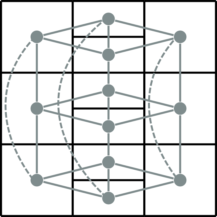
Figure 6: The cylindrical graph $\tilde{G}$ for $G=G(\bm{T}_{\langle 3,6,3\rangle})$. The new edges are dashed.

Consider now the graphs $G_{n}\mathrel{\mathop{:}}=G(\bm{T}^{n}_{(b,k)})$ for some $k\geqslant b\geqslant 4$ and $n\geqslant 1$. Let us define the cylindrical version $\tilde{G}_{n}$ of $G_{n}$ with the same vertex set, but additionally and edge from the top tile to the bottom tile in every column (see Figure 6). If we choose $\tilde{\rho}_{n}\in V(\tilde{G}_{n})$ according to the stationary measure on $\tilde{G}_{n}$, then clearly $\{(\tilde{G}_{n},\tilde{\rho}_{n})\}\Rightarrow(G_{b,k},\rho)$ as well.

Define also $L_{n}\mathrel{\mathop{:}}=L^{n}_{b,k}$. Because of Observation 3.4(b), the graph $\tilde{G}_{n}$ has vertical symmetry: Tiles within a column all have the same degree and, more specifically, have the same number of neighbors on the left and on the right. Let $\pi_{n}:V(G_{n})\to V(L_{n})$ denote the projection map and observe that

$$d_{\tilde{G}_{n}}(u,v)\geqslant d_{L_{n}}\!\left(\pi_{n}(u),\pi_{n}(v)\right),\qquad\forall u,v\in V(G_{n}).$$

Let $\{X^{(n)}_{t}\}$ denote the random walk on $\tilde{G}_{n}$ with $X^{(n)}_{0}=\tilde{\rho}_{n}$, and let $\{Y^{(n)}_{t}\}$ be the stationary random walk on $L_{n}$ defined in (3.10).

Note that, by construction, $\{\pi_{n}(X_{t}^{(n)})\}$ and $\{Y_{t}^{(n)}\}$ have the same law, and therefore

$$\operatorname*{\vvmathbb{E}}\left[d_{\tilde{G}_{n}}\left(X^{(n)}_{0},X^{(n)}_{T}\right)\right]\geqslant\operatorname*{\vvmathbb{E}}\left[d_{L_{n}}\left(Y^{(n)}_{0},Y^{(n)}_{T}\right)\right].$$ (3.15)

With this in hand, we can establish speed lower bounds in the limit $(G_{b,k},\rho)$.

Proof of Theorem 3.10.

Observe that (3.15) in conjunction with Lemma 3.16 gives, for every $T\leqslant c_{k}(\mathrm{diam}(\tilde{G}_{n})/2)^{\mathsf{d}_{w}(b,k)}$,

$$\operatorname*{\vvmathbb{E}}\left[d_{\tilde{G}_{n}}\!\left(X^{(n)}_{0},X^{(n)}_{T}\right)\right]\gtrsim_{k}T^{1/\mathsf{d}_{w}(b,k)}$$

Since $\{(\tilde{G}_{n},\rho_{n})\}\Rightarrow(G,\rho)$ by Lemma 3.9, it holds that if $\{X_{t}\}$ is the random walk on $G$ with $X_{0}=\rho$, then for all $T\geqslant 1$,

$$\operatorname*{\vvmathbb{E}}\left[d_{G}(X_{0},X_{T})\right]\gtrsim_{k}T^{1/\mathsf{d}_{w}(b,k)}.\qed$$

3.4 Annular resistances

We will establish Theorem 1.5 by proving the following.

Theorem 3.17.

For any $k\geqslant b\geqslant 4$, there is a constant $C=C(k)$ such that for $G=G_{b,k}$, almost surely

$$\mathsf{R}_{\mathrm{eff}}^{G}\left(B_{G}(\rho,R)\leftrightarrow V(G)\setminus B_{G}(\rho,2R)\right)\leqslant CR^{\log_{b}(\Gamma_{b,k})},\quad\forall R\geqslant 1.$$

To see that this yields Theorem 1.5, consider some $k\geqslant b^{2}$, corresponding to the restriction $\mathsf{d}_{g}(b,k)\geqslant 3$. Then for all positive integers $p\geqslant 1$, we have $\mathsf{d}_{g}(b^{p},k^{p})=\mathsf{d}_{g}(b,k)$ and recalling (3.4),

$$\lim_{p\to\infty}\log_{b^{p}}\!\left(\Gamma_{b^{p},k^{p}}\right)=-1\,.$$

To prove Theorem 3.17, it suffices to show the following.

Lemma 3.18.

For every $n\geqslant 1$, $k\geqslant b\geqslant 4$, there is a constant $C=C(k)$ such that for $G=G(\bm{T}^{n}_{(b,k)})$, we have

$$\mathsf{R}_{\mathrm{eff}}^{G}\left(B_{G}(x,R)\leftrightarrow V(G)\setminus B_{G}(x,2R)\right)\leqslant CR^{\log_{b}(\Gamma_{b,k})},\quad\forall x\in V(G),1\leqslant R\leqslant\mathrm{diam}(G)/C\,.$$

Proof.

Denote $\bm{T}\mathrel{\mathop{:}}=\bm{T}_{(b,k)}$. Consider some value $1\leqslant R\leqslant\mathrm{diam}(G)/C$, and define $h\mathrel{\mathop{:}}=\lfloor\log_{b}(R/3)\rfloor$.

Let $\mathcal{C}_{1},\ldots,\mathcal{C}_{b^{n}}$ denote the columns of $\bm{T}^{n}$ and writing $\bm{T}^{n}=\bm{T}^{n-h}\circ\bm{T}^{h}$, let us partition the columns into consecutive sets $\mathcal{D}_{1},\ldots,\mathcal{D}_{b^{n-h}}$ (as in the proof of Lemma 3.12), where $\mathcal{D}_{i}=\mathcal{C}_{(i-1)b^{h}+1}\cup\cdots\cup\mathcal{C}_{ib^{h}}$. For $1\leqslant i\leqslant b^{n-h}$, let $\beta_{i}$ denote the number of tiles in the $i$th column of $\bm{T}^{n-h}$ so that $\mathcal{D}_{i}$ consists of $\beta_{i}$ copies of $\bm{T}^{h}$ stacked vertically.

Fix some vertex $x\in V(G)$ and suppose that $x\in\mathcal{D}_{s}$ for some $1\leqslant s\leqslant b^{n-h}$. Denote $\Delta\mathrel{\mathop{:}}=9b$. By choosing $C$ sufficiently large, we can assume that $b^{n-h}>2\Delta$, so that either $s\leqslant b^{n-h}-\Delta$ or $s\geqslant 1+\Delta$. Let us assume that $s\leqslant b^{n-h}-\Delta$, as the other case is treated symmetrically. Define $t\mathrel{\mathop{:}}=\lceil s+2+6b\rceil$ so that $t-s\leqslant\Delta$, and

$$d_{G}(\mathcal{D}_{s},\mathcal{D}_{t})\geqslant b^{h}(t-s-1)\geqslant(t-s-1)\frac{R}{3b}>2R\,.$$ (3.16)

Denote $\xi\mathrel{\mathop{:}}=\gcd(\beta_{s},\beta_{s+1},\ldots,\beta_{t})$. We claim that

$$\xi\gtrsim_{k}\max(\beta_{s},\beta_{s+1},\ldots,\beta_{t})\,.$$ (3.17)

This follows because $\min(\beta_{i},\beta_{i+1})\mid\max(\beta_{i},\beta_{i+1})$ for all $1\leqslant i<b^{n}$ (cf. Observation 3.4(b)), and moreover the ratio $\max(\beta_{i},\beta_{i+1})/\min(\beta_{i},\beta_{i+1})$ is bounded by a function depending only on $k$. Since $t-s\lesssim_{k}1$, this verifies (3.17).

Denote $\hat{\mathcal{D}}\mathrel{\mathop{:}}=\mathcal{D}_{s}\cup\cdots\cup\mathcal{D}_{t}$. One can verify that $\hat{\mathcal{D}}$ is a vertical stacking of $\xi$ copies of $\hat{\bm{T}}\mathrel{\mathop{:}}=\bm{T}_{\langle\beta_{s}/\xi,\ldots,\beta_{t}/\xi\rangle}\circ\bm{T}^{h}$, and Corollary 2.15 implies that

$$\rho(\hat{\bm{T}})\lesssim_{k}\rho(\bm{T}^{h})\lesssim\Gamma_{b,k}^{h}\,,$$ (3.18)

with the final inequality being the content of Lemma 3.7.

Let $\hat{\bm{A}}$ be the copy of $\hat{\bm{T}}$ that contains $x$, and let $\bm{S}$ be the copy of $\bm{T}^{h}$ in $\bm{T}^{n}=\bm{T}^{n-h}\circ\bm{T}^{h}$ that contains $x$. Since $\xi$ divides $\beta_{s}$, it holds that $\bm{S}\subseteq\hat{\bm{A}}$ and $\mathscr{L}(\bm{S})\subseteq\mathscr{L}(\hat{\bm{A}})$. We further have

$$|\mathscr{L}(\hat{\bm{A}})|=|\mathscr{L}(\hat{\bm{T}})|=(\beta_{s}/\xi)|\mathscr{L}(\bm{T}^{h})|=(\beta_{s}/\xi)|\mathscr{L}(\bm{S})|\lesssim_{k}|\mathscr{L}(\bm{S})|\,.$$

This yields

$$\mathsf{R}_{\mathrm{eff}}^{G}(\vvmathbb{1}_{\mathscr{L}(\bm{S})}/|\mathscr{L}(\bm{S})|\leftrightarrow\mathscr{R}(\hat{\bm{A}}))\lesssim_{k}\mathsf{R}_{\mathrm{eff}}^{G}(\vvmathbb{1}_{\mathscr{L}(\hat{\bm{A}})}/|\mathscr{L}(\hat{\bm{A}})|\leftrightarrow\mathscr{R}(\hat{\bm{A}})),$$ (3.19)

where we have used the hybrid notation: For $s\in\ell_{1}(V)$,

$$\mathsf{R}_{\mathrm{eff}}^{G}(s\leftrightarrow U)\mathrel{\mathop{:}}=\inf\left\{\mathsf{R}_{\mathrm{eff}}^{G}(s,t):\operatorname{supp}(t)\subseteq U,\|t\|_{1}=\|s\|_{1}\right\}.$$

Therefore,

$$\mathsf{R}_{\mathrm{eff}}^{G}(\mathscr{L}(\bm{S})\leftrightarrow\mathscr{R}(\hat{\bm{A}})) \leqslant\mathsf{R}_{\mathrm{eff}}^{G}(\vvmathbb{1}_{\mathscr{L}(\bm{S})}/|\mathscr{L}(\bm{S})|\leftrightarrow\mathscr{R}(\hat{\bm{A}}))$$

$$\stackrel{{\scriptstyle\mathclap{\eqref{eq:eff-compare}}}}{{\lesssim_{k}}}\mathsf{R}_{\mathrm{eff}}^{G}(\vvmathbb{1}_{\mathscr{L}(\hat{\bm{A}})}/|\mathscr{L}(\hat{\bm{A}})|\leftrightarrow\mathscr{R}(\hat{\bm{A}}))=\rho(\hat{\bm{T}})\stackrel{{\scriptstyle\eqref{eq:hatT}}}{{\lesssim_{k}}}\Gamma_{b,k}^{h}\,.$$

Since $\mathrm{diam}_{G}(\bm{S})\leqslant 3b^{h}\leqslant R$ and $x\in\bm{S}$, it holds that $\bm{S}\subseteq B_{G}(x,R)$. On the other hand, since $x\in\bm{S}$, (3.16) shows that $B_{G}(x,2R)\cap\mathscr{R}(\hat{\bm{A}})=\emptyset$. We conclude that

$$\mathsf{R}_{\mathrm{eff}}^{G}(B_{G}(x,R)\leftrightarrow V(G)\setminus B_{G}(x,2R))\leqslant\mathsf{R}_{\mathrm{eff}}^{G}(\mathscr{L}(\bm{S})\leftrightarrow\mathscr{R}(\hat{\bm{A}}))\lesssim_{k}\Gamma^{h}_{b,k}\lesssim_{k}R^{\log_{b}(\Gamma_{b,k})},$$

as desired. ∎

3.5 Complements of balls are connected

Let us finally prove Theorem 1.4. Recall the setup from Section 3.3.3: We take $k\geqslant b\geqslant 4$, define $G_{n}=G(\bm{T}^{n}_{(b,k)})$, and use $(\tilde{G}_{n},\tilde{\rho}_{n})$ to denote the cylindrical version, which satisfies $\{(\tilde{G}_{n},\tilde{\rho}_{n})\}\Rightarrow(G_{b,k},\rho)$.

Partition the vertices of $\tilde{G}_{n}$ into columns $\mathcal{C}_{1},\ldots,\mathcal{C}_{b^{n}}$ in the natural way (as was done in Section 3.3 and Section 3.4). In what follows, we say that a set $S\subseteq V(\tilde{G}_{n})$ is connected to mean that $\tilde{G}_{n}[S]$ is a connected graph.

Definition 3.19.

Say that a set of vertices $U\subseteq V(\tilde{G}_{n})$ is vertically convex if for all $1\leqslant i\leqslant b^{n}$, either $U\cap\mathcal{C}_{i}=\emptyset$ or $U\cap\mathcal{C}_{i}$ is connected.

Observation 3.20.

Consider a connected set $U\subseteq\mathcal{C}_{i}$ for some $1\leqslant i\leqslant b^{n}$. Then for $1\leqslant i^{\prime}\leqslant b^{n}$ with $|i-i^{\prime}|\leqslant 1$, the set $B_{\tilde{G}_{n}}(U,1)\cap\mathcal{C}_{i^{\prime}}$ is connected.

Momentarily, we will argue that balls in $\tilde{G}_{n}$ are vertically convex.

Lemma 3.21.

Consider any $A\in\bm{T}$ and $R\geqslant 0$. It holds that $B_{\tilde{G}_{n}}(A,R)$ is vertically convex.

With this lemma in hand, it is easy to establish the following theorem which, in conjunction with Lemma 3.9, implies Theorem 1.4.

Theorem 3.22.

Almost surely, the complement of every ball in $G_{b,k}$ is connected.

Proof.

Since $\{(\tilde{G}_{n},\tilde{\rho}_{n})\}\Rightarrow G_{b,k}$, it suffices to argue that for every $n\geqslant 1$, $x\in V(\tilde{G}_{n})$, and $R\leqslant b^{n}/3$, the set $U\mathrel{\mathop{:}}=V(\tilde{G}_{n})\setminus B_{\tilde{G}_{n}}(x,R)$ is connected.

By Lemma 3.21, it holds that $B_{\tilde{G}_{n}}(x,R)$ is vertically convex. Since the complement of a vertically convex set is vertically convex (given that every column in $\tilde{G}_{n}$ is isomorphic to a cycle), $U$ is vertically convex as well. To argue that $U$ is connected, it therefore suffices to prove that there is a path from $\mathscr{L}(\bm{T}^{n}_{(b,k)})$ to $\mathscr{R}(\bm{T}^{n}_{(b,k)})$ in $\tilde{G}_{n}[U]$.

In fact, the tiles in $\bm{T}^{n}_{(b,k)}$ have height at most $b^{-n}$, and therefore the projection of $K\mathrel{\mathop{:}}=\left\llbracket B_{\tilde{G}_{n}}(x,R)\right\rrbracket$ onto $\{0\}\times[0,1]$ has length at most $(2R+1)b^{-n}<1$. Hence there is some height $h\in[0,1]$ such that a horizontal line $\ell$ at height $h$ does not intersect $K$. The set of tiles $\{A\in V(\tilde{G}_{n}):\ell\cap\left\llbracket A\right\rrbracket\neq\emptyset\}$ therefore contains a path from $\mathscr{L}(\bm{T}^{n}_{(b,k)})$ to $\mathscr{R}(\bm{T}^{n}_{(b,k)})$ that is contained in $\tilde{G}_{n}[U]$, completing the proof. ∎

We are left to prove Lemma 3.21. To state the next lemma more cleanly, let us denote $\mathcal{C}_{0}=\mathcal{C}_{b^{n}+1}=\emptyset$.

Lemma 3.23.

Consider $1\leqslant i\leqslant b^{n}$ and let $U\subseteq\mathcal{C}_{i-1}\cup\mathcal{C}_{i}\cup\mathcal{C}_{i+1}$ be a connected, vertically convex subset of vertices. Then $B_{\tilde{G}_{n}}(U,1)\cap\mathcal{C}_{i}$ is connected as well.

Proof.

For $i^{\prime}\in\{i-1,i,i+1\}$, denote $U_{i^{\prime}}\mathrel{\mathop{:}}=U\cap C_{i^{\prime}}$. Clearly we have

$$B_{\tilde{G}_{n}}(U,1)=B_{\tilde{G}_{n}}(U_{i-1},1)\cup B_{\tilde{G}_{n}}(U_{i},1)\cup B_{\tilde{G}_{n}}(U_{i+1},1)\,.$$

If $U_{i}=\emptyset$, then as $U$ is connected it should be that either $U=U_{i-1}$ or $U=U_{i+1}$, and in either case the claim follows by Observation 3.20.

Now suppose $U_{i}\neq\emptyset$, and consider some $i^{\prime}\in\{i-1,i+1\}$ such that $U_{i^{\prime}}\neq\emptyset$. Then Observation 3.20 implies that $B_{\tilde{G}_{n}}(U_{i^{\prime}},1)\cap\mathcal{C}_{i}$ is connected. Furthermore, since $U$ is connected, it holds that $B_{\tilde{G}_{n}}(U_{i^{\prime}},1)\cap U_{i}\neq\emptyset$. Now, as we know that $U_{i}$ is connected by the assumed vertical convexity of $U$, we obtain that $B_{\tilde{G}_{n}}(U,1)\cap\mathcal{C}_{i}$ is connected, completing the proof. ∎

Proof of Lemma 3.21.

We proceed by induction on $R$, where the base case $R=0$ is trivial, so consider $R\geqslant 1$. Fix some $i\in\{1,2,\ldots,b^{n}\}$, and suppose $B_{\tilde{G}_{n}}(A,R)\cap\mathcal{C}_{i}\neq\emptyset$. Denote

$$U\mathrel{\mathop{:}}=B_{\tilde{G}_{n}}(A,R-1)\cap(\mathcal{C}_{i-1}\cup\mathcal{C}_{i}\cup\mathcal{C}_{i+1})\,.$$

Clearly we have $B_{\tilde{G}_{n}}(A,R)\cap\mathcal{C}_{i}=B_{\tilde{G}_{n}}(U,1)\cap\mathcal{C}_{i}$. The set $U$ is manifestly connected and, by the induction hypothesis, is also vertically convex. Thus from Lemma 3.23, it follows that $B_{\tilde{G}_{n}}(U,1)\cap\mathcal{C}_{i}$ is connected as well. We conclude that $B_{\tilde{G}_{n}}(A,R)$ is vertically convex, completing the proof. ∎

Acknowledgements

We thank Shayan Oveis Gharan and Austin Stromme for many useful preliminary discussions, Omer Angel and Asaf Nachmias for sharing with us their construction of a graph with asymptotic $(3-\varepsilon)$-dimensional volume growth on which the random walk has diffusive speed, and Itai Benjamini for emphasizing many of the questions addressed here. We also thank the anonymous referees for very useful comments. This research was partially supported by NSF CCF-1616297 and a Simons Investigator Award.

References

[ADJ97]
Jan Ambjørn, Bergfinnur Durhuus, and Thordur Jonsson.
Quantum geometry.
Cambridge Monographs on Mathematical Physics. Cambridge University
Press, Cambridge, 1997.
A statistical field theory approach.
[AL07]
David Aldous and Russell Lyons.
Processes on unimodular random networks.
Electron. J. Probab., 12:no. 54, 1454–1508, 2007.
[Ang03]
O. Angel.
Growth and percolation on the uniform infinite planar triangulation.
Geom. Funct. Anal., 13(5):935–974, 2003.
[Bar98]
Martin T. Barlow.
Diffusions on fractals.
In Lectures on probability theory and statistics
(Saint-Flour, 1995), volume 1690 of Lecture Notes in Math., pages
1–121. Springer, Berlin, 1998.
[BC12]
Itai Benjamini and Nicolas Curien.
Ergodic theory on stationary random graphs.
Electron. J. Probab., 17:no. 93, 20 pp., 2012.
[BC13]
Itai Benjamini and Nicolas Curien.
Simple random walk on the uniform infinite planar quadrangulation:
subdiffusivity via pioneer points.
Geom. Funct. Anal., 23(2):501–531, 2013.
[Ben13]
Itai Benjamini.
Coarse geometry and randomness, volume 2100 of Lecture
Notes in Mathematics.
Springer, Cham, 2013.
Lecture notes from the 41st Probability Summer School held in
Saint-Flour, 2011, Chapter 5 is due to Nicolas Curien, Chapter 12 was written
by Ariel Yadin, and Chapter 13 is joint work with Gady Kozma, École
d’Été de Probabilités de Saint-Flour. [Saint-Flour Probability
Summer School].
[BK02]
Mario Bonk and Bruce Kleiner.
Quasisymmetric parametrizations of two-dimensional metric spheres.
Invent. Math., 150(1):127–183, 2002.
[BP11]
Itai Benjamini and Panos Papasoglu.
Growth and isoperimetric profile of planar graphs.
Proc. Amer. Math. Soc., 139(11):4105–4111, 2011.
[BS01]
Itai Benjamini and Oded Schramm.
Recurrence of distributional limits of finite planar graphs.
Electron. J. Probab., 6:no. 23, 13 pp., 2001.
[CRR+97]
Ashok K. Chandra, Prabhakar Raghavan, Walter L. Ruzzo, Roman Smolensky, and
Prasoon Tiwari.
The electrical resistance of a graph captures its commute and cover
times.
Comput. Complexity, 6(4):312–340, 1996/97.
[GN13]
Ori Gurel-Gurevich and Asaf Nachmias.
Recurrence of planar graph limits.
Ann. of Math. (2), 177(2):761–781, 2013.
[KM08]
Takashi Kumagai and Jun Misumi.
Heat kernel estimates for strongly recurrent random walk on random
media.
J. Theoret. Probab., 21(4):910–935, 2008.
[Lee17]
James R. Lee.
Conformal growth rates and spectral geometry on distributional limits
of graphs.
Preprint at
arXiv:math/1701.01598, 2017.
[LP16]
Russell Lyons and Yuval Peres.
Probability on Trees and Networks.
Cambridge University Press, New York, 2016.
Preprint at http://pages.iu.edu/~rdlyons/.