Scattering of a Klein-Gordon particle by a smooth barrier

Abstract

We present the study of the one-dimensional Klein-Gordon equation by a smooth barrier. The scattering solutions are given in terms of the Whittaker $M_{\kappa,\mu}(x)$ function. The reflection and transmission coefficients are calculated in terms of the energy, the height and the smoothness of the potential barrier. For any value of the smoothness parameter we observed transmission resonances.

Keywords: Hypergeometric functions, Klein-Gordon equation, Scattering theory.

1 Introduction

In this article we computed the scattering solutions of the one-dimensional Klein-Gordon equation in presence of a smooth barrier. This is a mathematical interesting problem because the solutions of the Klein-Gordon equation are given in terms of the Whittaker $M_{\kappa,\mu}(x)$ function, whose asymptotic behavior is well-known.

This smooth barrier is a short-range potential which presents scattering states. This potential is interesting because varying the smoothness of the curve can be represented from the potential barrier to the cusp potential barrier, in all cases we observed transmission resonances. These potential barriers have applications in several topics of the solid state physics.

The Klein-Gordon equation is used to describe spin-0 particles. This equation have been widely study in the literature for different physical systems both time-independent [1, 2, 3, 4, 5, 6, 7, 8, 9, 10, 11, 12, 13] and time-dependent [14, 15, 16, 17] Klein-Gordon equation. The analytical solution of the time-independent Klein-Gordon equation for different potentials has been caused of a lot of interest in recent years, for both bound states [2, 3, 6, 9, 12] and scattering solutions [1, 4, 5, 7, 8, 9, 10, 11, 13]. It has allowed the understanding of several physical phenomena of Relativistic Quantum Mechanics such as the antiparticle bound state [18, 19], transmission resonances [1, 4, 5], and superradiance [20, 7, 21, 22].

This article is organized as follow. In section 2, we present the one-dimensional Klein-Gordon equation. In section 3, we present the smooth barrier. In section 4 we study the solutions for scattering states, and calculate the transmission and reflection coefficients. The discussion of our results are given in section 5. Finally, in section 6 we give the concluding remarks.

2 The Klein-Gordon equation

The Klein-Gordon equation for free particles, in natural units $\hbar=c=m=1$, is given by [23],

$$\hat{p}^{\mu}\hat{p}_{\mu}\varphi=\varphi,$$ (1)

being $\hat{p}^{\mu}=i\left(\dfrac{\partial}{\partial t},-\vec{\nabla}\right)$, Eq. (1) becomes:

$$\left(\Box+1\right)\varphi=0.$$ (2)

We need to solve the Klein-Gordon equation interacting with a spatially one-dimensional potential, then we start finding the form of the Klein-Gordon equation with the interaction of an electromagnetic field.

The electromagnetic field is described by the four-vector [23]:

$$A^{\mu} = (A_{0},\vec{A}),$$ (3)

$$A_{\mu} = \eta_{\mu\nu}A^{\nu}=(A_{0},-\vec{A}),$$ (4)

where $\eta_{\mu\nu}=\textnormal{diag}(1,-1)$.

The minimal coupling of the electromagnetic field is expressed in the form,

$$\hat{A}^{\mu} \rightarrow \hat{p}^{\mu}-eA^{\mu},$$ (5)

$$\hat{A}_{\mu} \rightarrow \hat{p}_{\mu}-eA_{\mu}.$$ (6)

The one-dimensional Klein-Gordon equation minimally coupled to a vector potential $A^{\mu}$ can be written as [23]:

$$(\hat{p}^{\mu}-eA^{\mu})(\hat{p}_{\mu}-eA_{\mu})\varphi=\varphi.$$ (7)

Consider a spatially one-dimensional potential $eA_{0}=V(x)$, $\vec{A}=0$, and a stationary solution of the Klein-Gordon equation $\varphi(x,t)=\phi(x)e^{-iEt}$, Eq. (7) can be written as:

$$\frac{\mathrm{d}^{2}\phi(x)}{\mathrm{d}x^{2}}+\left\{[E-V(x)]^{2}-1\right\}\phi(x)=0,$$ (8)

where $E$ is the energy of the particle.

3 The smooth barrier

The smooth barrier is given by:

$$V(x)=\left\{\begin{array}[]{ll}\quad V_{0}e^{\nicefrac{{(x-x_{0})}}{{a}}},\quad\textnormal{for}\quad x<x_{0},\\ \quad V_{0},\quad\textnormal{for}\quad x_{0}\leq x\leq 0,\\ \quad V_{0}e^{-\nicefrac{{x}}{{a}}},\quad\textnormal{for}\quad x>0,\end{array}\right.$$ (9)

where $V_{0}$ represents the height of the barrier and $a$ gives the smoothness of the curve. The form of the potential (9) is showed in the Fig. (1). From Fig. 1 we can note that the smooth barrier reduces to the square potential barrier for $a\rightarrow 0$. Also this potential reduces to the cusp potential barrier for $a\gg 0$ and $x_{0}=0$.

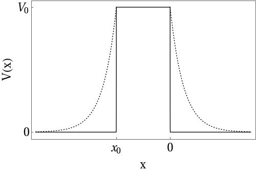
Figure 1: Smooth barrier for $V_{0}=2$ with $a=0.5$ (dotted line) and square potential barrier for $a=0.001$ (solid line).

4 Scattering States

4.1 Scattering solutions for $x<x_{0}$

The scattering solutions for $x<x_{0}$ are obtained by solving the differential equation

$$\frac{\mathrm{d}^{2}\phi_{\textnormal{I}}(x)}{\mathrm{d}x^{2}}+\left\{\left[E-V_{0}e^{\nicefrac{{(x-x_{0})}}{{a}}}\right]^{2}-1\right\}\phi_{\textnormal{I}}(x)=0.$$ (10)

On making the chang of variable $y=2iaV_{0}e^{\nicefrac{{(x-x_{0})}}{{a}}}$, Eq. (10) becomes

$$y\frac{\mathrm{d}}{\mathrm{d}y}\left(y\frac{\phi_{\textnormal{I}}}{\mathrm{d}y}\right)-\left[\left(iaE-\nicefrac{{y}}{{2}}\right)^{2}+a^{2}\right]\phi_{\textnormal{I}}=0.$$ (11)

Putting $\phi_{\textnormal{I}}=y^{-\nicefrac{{1}}{{2}}}f(y)$ we obtain the Whittaker differential equation

$$f(y)^{\prime\prime}+\left[-\frac{1}{4}\textasciiacute+\frac{iaE}{y}+\frac{\nicefrac{{1}}{{4}}-a^{2}(1-E^{2})}{y^{2}}\right]f(y)=0,$$ (12)

which general solution is given by

$$f(y)=c_{1}M_{\kappa,\mu}(y)+d_{1}W_{\kappa,\mu}(y),$$ (13)

where $M_{\kappa,\mu}(y)$, $W_{\kappa,\mu}(y)$ are the Whittaker functions, $\kappa=iaE$ and $\mu=i\sqrt{E^{2}-1}a$. Then the solution to the Eq. (11) is given by,

$$\phi_{\textnormal{I}}(y)=c_{1}y^{-\nicefrac{{1}}{{2}}}M_{\kappa,\mu}(y)+d_{1}y^{-\nicefrac{{1}}{{2}}}W_{\kappa,\mu}(y).$$ (14)

In terms of the variable $x$, Eq. (14) becomes

$$\phi_{\textnormal{I}}(x) = c_{1}(2iaV_{0})^{(-\nicefrac{{1}}{{2}})}e^{-\nicefrac{{(x-x_{0})}}{{2a}}}M_{\kappa,\mu}\left[2iaV_{0}e^{\nicefrac{{(x-x_{0})}}{{a}}}\right]$$ (15)

$$+ d_{1}(2iaV_{0})^{(-\nicefrac{{1}}{{2}})}e^{-\nicefrac{{(x-x_{0})}}{{2a}}}W_{\kappa,\mu}\left[2iaV_{0}e^{\nicefrac{{(x-x_{0})}}{{a}}}\right].$$

Because the asymptotic behavior of the Whittaker functions we only keep the solutions with the $M_{\kappa,\mu}(x)$ function. Then, from Eq. (15), the incident and reflected waves are,

$$\phi_{\textnormal{inc}}(x) = c_{1}(2iaV_{0})^{(-\nicefrac{{1}}{{2}})}e^{-\nicefrac{{(x-x_{0})}}{{2a}}}M_{\kappa,\mu}\left[2iaV_{0}e^{\nicefrac{{(x-x_{0})}}{{a}}}\right],$$

$$\phi_{\textnormal{ref}}(x) = b_{1}(2iaV_{0})^{(-\nicefrac{{1}}{{2}})}e^{-\nicefrac{{(x-x_{0})}}{{2a}}}M_{\kappa,-\mu}\left[2iaV_{0}e^{\nicefrac{{(x-x_{0})}}{{a}}}\right],$$ (16)

which are solutions of the differential equation (10).

4.2 Scattering solutions for $x_{0}\leq x\leq 0$

The scattering solutions for $x_{0}<x<0$ are obtained by solving the differential equation

$$\frac{\mathrm{d}^{2}\phi_{\textnormal{II}}(x)}{\mathrm{d}x^{2}}+\left[\left(E-V_{0}\right)^{2}-1\right]\phi_{\textnormal{II}}(x)=0,$$ (17)

Eq. (17) has the general solution

$$\phi_{\textnormal{II}}(x)=b_{2}\,e^{-iqx}+c_{2}\,e^{iqx},$$ (18)

where $q=\sqrt{\left(E-V_{0}\right)^{2}-1}$.

4.3 Scattering solutions for $x>0$

The scattering solutions for $x>0$ are obtained by solving the differential equation

$$\frac{\mathrm{d}^{2}\phi_{\textnormal{III}}(x)}{\mathrm{d}x^{2}}+\left[\left(E-V_{0}e^{-x/a}\right)^{2}-1\right]\phi_{\textnormal{III}}(x)=0.$$ (19)

On making the change of variable $z=2iaV_{0}e^{-\nicefrac{{x}}{{a}}}$, Eq. (19) becomes

$$z\frac{\mathrm{d}}{\mathrm{d}z}\left(z\frac{\phi_{\textnormal{III}}}{\mathrm{d}z}\right)-\left[\left(iaE-\nicefrac{{z}}{{2}}\right)^{2}+a^{2}\right]\phi_{\textnormal{III}}=0.$$ (20)

Putting $\phi_{\textnormal{III}}=z^{-\nicefrac{{1}}{{2}}}g(z)$ we obtain the Whittaker differential equation

$$g(z)^{\prime\prime}+\left[-\frac{1}{4}+\frac{iaE}{z}+\frac{\nicefrac{{1}}{{4}}-a^{2}(1-E^{2})}{z^{2}}\right]g(z)=0,$$ (21)

which solution is given by

$$g(z)=c_{3}M_{\kappa,-\mu}(z)+d_{3}W_{\kappa,-\mu}(z),$$ (22)

Finally, the solution of Eq. (20) becomes

$$\phi_{\textnormal{III}}(z)=c_{3}z^{-\nicefrac{{1}}{{2}}}M_{\kappa,-\mu}(z)+d_{3}z^{-\nicefrac{{1}}{{2}}}W_{\kappa,-\mu}(z),$$ (23)

In terms of the variable $x$, (23) becomes

$$\phi_{\textnormal{III}}(x) = b_{3}(2iaV_{0})^{(-\nicefrac{{1}}{{2}})}e^{\nicefrac{{x}}{{2a}}}M_{\kappa,-\mu}\left(2iaV_{0}e^{\nicefrac{{-x}}{{a}}}\right)$$ (24)

$$+ d_{3}(2iaV_{0})^{(-\nicefrac{{1}}{{2}})}e^{\nicefrac{{x}}{{2a}}}W_{\kappa,-\mu}\left(2iaV_{0}e^{\nicefrac{{-x}}{{a}}}\right).$$

From Eq. (4.3) the transmitted wave is:

$$\phi_{\textnormal{trans}}(x)=b_{3}(2iaV_{0})^{(-\nicefrac{{1}}{{2}})}e^{\nicefrac{{x}}{{2a}}}M_{\kappa,-\mu}\left(2iaV_{0}e^{\nicefrac{{-x}}{{a}}}\right).$$

4.4 Transmission and reflection coefficients

For compute the transmission and reflection coefficient we need to use the definition of the electrical current. The electrical current density for the one-dimensional Klein-Gordon equation (8) is defined as

$$j^{\mu}=\frac{i}{2}\left(\phi^{*}\,\partial^{\mu}\phi-\phi\,\partial^{\mu}\phi^{*}\right).$$ (25)

The current as $x\rightarrow-\infty$ can be descomposed as $j_{\textnormal{L}}=j_{\textnormal{in}}-j_{\textnormal{refl}}$ where $j_{\textnormal{in}}$ is the incident current and $j_{\textnormal{refl}}$ is the reflected one. Analogounls we have that, on the right side, as $x\rightarrow\infty$ the current is $j_{\textnormal{R}}=j_{\textnormal{trans}}$, where $j_{\textnormal{trans}}$ is the transmitted current.

Using The reflection coefficient $R$, and the transmission coefficient $T$, are calculated by

$$R=\frac{j_{\textnormal{refl}}}{j_{\textnormal{inc}}},$$ (26)

$$T=\frac{j_{\textnormal{trans}}}{j_{\textnormal{inc}}},$$ (27)

for which we need to identify the incident, reflected and transmitted wave. The quantities $R$ and $T$ are not independet, they are related via the unitary condition $R+T=1$.

Using the asymptotic behavior of the Whittaker function $M_{\kappa,\mu}\rightarrow e^{-\nicefrac{{y}}{{2}}}y^{\nicefrac{{1}}{{2}}+\mu}$, as $y\rightarrow 0$ [24], we can write the incoming solution, the reflected solution and the transmitted solutions like a plane wave.

From Eq. (15), as $x\rightarrow-\infty$, the incident and reflected waves are given by

$$\phi_{\textnormal{inc}}(x)=c_{1}\,(2iaV_{0})^{\mu}e^{i\sqrt{E^{2}-1}x},$$ (28)

$$\phi_{\textnormal{ref}}(x)=b_{1}\,(2iaV_{0})^{-\mu}e^{-i\sqrt{E^{2}-1}x},$$ (29)

and from Eq. (4.3) as $x\rightarrow\infty$ the transmitted wave has the form,

$$\phi_{\textnormal{trans}}(x)\rightarrow b_{3}\,(2iaV_{0})^{-\mu}e^{i\sqrt{E^{2}-1}x}.$$ (30)

Then

$$R=\left|\dfrac{(2iaV_{0})^{-\mu}}{(2iaV_{0})^{\mu}}\right|^{2}\left|\dfrac{b_{1}}{c_{1}}\right|^{2},$$ (31)

$$T=\left|\dfrac{(2iaV_{0})^{-\mu}}{(2iaV_{0})^{\mu}}\right|^{2}\left|\dfrac{b_{3}}{c_{1}}\right|^{2}.$$ (32)

In order to find $R$ and $T$, the wave functions and their first derivatives must be matched at $x=x_{0}$ and $x=0$. The coefficients $b_{1}$ and $b_{3}$ are calculated numerically in terms of $c_{1}$ from the following system of equations,

$$b_{1}\,M_{\kappa,\mu}(2iaV_{0})+c_{1}\,M_{\kappa,-\mu}(2iaV_{0})=b_{2}\,e^{-iqx_{0}}+c_{2}\,e^{iqx_{0}},$$ (33)

$$b_{1}\left[\left(-\dfrac{1}{2a}+iV_{0}+\dfrac{\kappa}{a}\right)M_{\kappa,\mu}(2iaV_{0})-\dfrac{1}{a}\left(\dfrac{1}{2}+\mu+\kappa\right)M_{\kappa+1,-\mu}(2iaV_{0})\right]+$$

$$c_{1}\left[\left(-\dfrac{1}{2a}+iV_{0}-\dfrac{\kappa}{a}\right)M_{\kappa,-\mu}(2iaV_{0})+\dfrac{1}{a}\left(\dfrac{1}{2}-\mu+\kappa\right)M_{\kappa+1,-\mu}(2iaV_{0})\right]$$

$$=-b_{2}\,qe^{-iqx_{0}}+c_{2}\,qe^{irx_{0}},$$ (34)

$$b_{2}\,+c_{2}\,=b_{3}\,M_{\kappa,-\mu}(2iaV_{0}),$$ (35)

$$ib_{2}\,q+ic_{2}\,q=b_{3}\left[\left(\dfrac{1}{2a}-iV_{0}+\dfrac{\kappa}{a}\right)M_{\kappa,-\mu}(2iaV_{0})-\dfrac{1}{a}\left(\dfrac{1}{2}-\mu+\kappa\right)M_{\kappa+1,-\mu}(2iaV_{0})\right].$$ (36)

5 Results and discussion

Fig. (2) shows the transmission and reflection coefficients for $x_{0}=-1$, $a=0.5$ and $E=2$ respect to the height of the barrier $V_{0}$. Fig. (3) shows the transmission and reflection coefficients for $x_{0}=-2$, $a=0.5$ and $E=2$ respect to the height of the barrier $V_{0}$. When the value of $x_{0}$ increases, more peaks appear in the same range of $V_{0}$. Using the values $a=0.5$ with $x_{0}=0$ in Fig. (4) and $a=0.001$ in Fig. (5) we recover the results obtained by the cusp potential barrier and the square potential barrier, respectively. In all cases we observed transmission resonances. The relation $T+R=1$ also is satisfied.

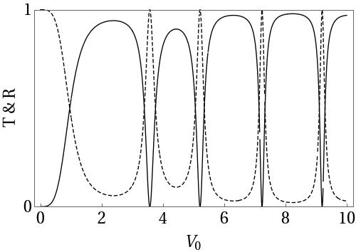
Figure 2: Transmission and reflection coefficients in function of the height of the barrier $V_{0}$ for $x_{0}=-1$, $a=0.5$ and $E=2$. The dashed line represents the transmission coefficient, and the solid line represents the reflection coefficient.

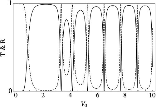
Figure 3: Transmission and reflection coefficients in function of the height of the barrier $V_{0}$ for $x_{0}=-2$, $a=0.5$ and $E=2$. The dashed line represents the transmission coefficient, and the solid line represents the reflection coefficient.

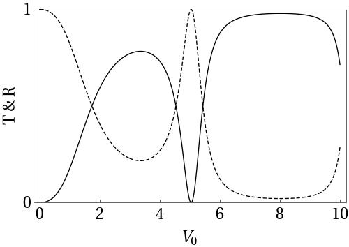
Figure 4: Transmission and reflection coefficients in function of the height of the barrier $V_{0}$ for $x_{0}=0$, $a=0.5$ and $E=2$. The dashed line represents the transmission coefficient, and the solid line represents the reflection coefficient.

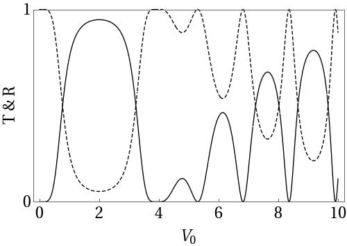
Figure 5: Transmission and reflection coefficients in function of the height of the barrier $V_{0}$ for $x_{0}=-2$, $a=0.001$ and $E=2$. The dashed line represents the transmission coefficient, and the solid line represents the reflection coefficient.

In the non-relativistic limit the Klein-Gordon equation reduces to the Schödinger equation [23]. We wish to compare the scattering solutions of the Schrodinger equation with those of the Klein Gordon equation for the square potential barrier.

For the square potential barrier showed in Fig. 1 (solid line), the reflection $R$ and transmission $T$ coefficients are obtained by:

$$R_{\textnormal{barrier}}=\dfrac{(k_{1}^{2}-k_{2}^{2})^{2}\sin^{2}\left(k_{2}x_{0}\right)}{4k_{1}^{2}k_{2}^{2}+(k_{1}^{2}-k_{2}^{2})^{2}\sin^{2}\left(k_{2}x_{0}\right)}.$$ (37)

$$T_{\textnormal{barrier}}=\dfrac{4k_{1}^{2}k_{2}^{2}}{4k_{1}^{2}k_{2}^{2}+(k_{1}^{2}-k_{2}^{2})^{2}\sin^{2}\left(k_{2}x_{0}\right)},$$ (38)

where $k_{1}=\sqrt{2E}$, $k_{2}=\sqrt{2(E-V_{0})}$ for the Schödinger equation and $k_{1}=\sqrt{E^{2}-1}$, $k_{2}=\sqrt{(E-V_{0})^{2}-1}$ for the Klein-Gordon equation.

In Figs. 6 and 7 we illustred the behaviour of the reflection and transmission coefficients in both cases. We can observed that for the Klein-Gordon equation more peaks appears in the transmission coefficient that for the Schödinger equation. In both cases the relation $T+R=1$ is accomplished.

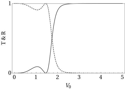
Figure 6: The reflection $R$ and transmission $T$ coefficients varying energy $V_{0}$ of the Schödinger equation with the square potential barrier for $E=3$ and $x_{0}=-3$. The dashed line represents the transmission coefficient, and the solid line represents the reflection coefficient.

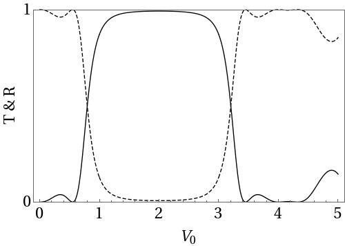
Figure 7: The reflection $R$ and transmission $T$ coefficients varying energy $V_{0}$ of the Klein-Gordon equation with the square potential barrier for $E=3$ and $x_{0}=-3$. The dashed line represents the transmission coefficient, and the solid line represents the reflection coefficient.

6 Conclusions

In this paper we have studied the scattering solutions of the Klein-Gordon equation by a smooth barrier. We have calculated the transmission $T$ and reflection $R$ coefficients in function of the height of the potential $V_{0}$ for three different widths of the barrier. For certain values of the smoothness and weight of the potential barrier we recover the results for the cusp potential [4] and for the square potential barrier [23, 25]. In all cases we observe transmission resonances and the relationship $T+R=1$ is accomplished. For future research we are going to consider the bound-states solutions of this smooth potential barrier.

References

- [1] C. Rojas and V. M. Villalba. Scattering of a Klein-Gordon particle by a Woods-Saxon potential. Phys. Rev. A, 71:052101, 2005.
- [2] C. Rojas and V. M. Villalba. The Klein-Gordon equation with the Woods-Saxon potential well. Rev. Mex. Fis, 52:127, 2006.
- [3] V. M. Villalba and C. Rojas. Bound states of the Klein-Gordon equation in the presence of short range potentials. Int. J. Mod. Phys. A, 21:313, 2006.
- [4] V. M. Villalba and C. Rojas. Scattering of a relativistic scalar particle by a cusp potential. Phys. Lett. A, 362:21, 2007.
- [5] V. M. Villalba and L. A. GonzálezDíaz. Resonant states in an attractive one-dimensional cusp potential. Phys. Scr., 75:645, 2007.
- [6] G. Chen, Z.-D. Chena and Z.-M. Loua. Exact bound state solutions of the s-wave Klein-Gordon equation with the generalized Hulthén potential. Phys. Lett. A, 367:498, 2007.
- [7] C. Rojas. Scattering of a relativistic particle by a hyperbolic tangent potential. Can. J. Phys., 99:1, 2014.
- [8] C. Rojas. Scattering solutions of the kleingordon equation for a step potential with hyperbolic tangent potential. Mod. Phys. Lett. A, 29:1450146, 2014.
- [9] H. Hassanabadi, S. Zarrinkamar and E. Maghsoodi. Cusp interation in minimal length quantum mechanics. Body Syst., 55:255, 2014.
- [10] A. N. Ikok, H. Hassanabadi, N. Salehi, H. P. Obong and M. C. Onyeaju. Scattering states of cusp potential in minimal length dirac equation. Indian J. Phys, 89:1221, 2015.
- [11] M. Chabab, A. El Batoul, H. Hassanabadi, M. Oulne and S. Zare. Scattering states of dirac particle equation with position-dependent mass under the cusp potential. Eur. Phys. J. Plus, 131:2016, 2016.
- [12] Wen-Du Li and Wu-Sheng Dai. Exact solution of inversesquareroot potential . Ann. Phys., 373:207, 2016.
- [13] E. J. Aquino Curi, L. B. Castro and A. S. de Castro. Proper treatment of scalar and vector exponential potentials in the klein-gorodon equations: Scattering and bound states. Eur. Phys. J. Plus, 134:248, 2019.
- [14] D. J. Rowan and G. Stephenson. Solutions of the time-dependent klein-gordon equation in a schwarzschild background space. J. Phys. A: Math. Gen., 9:1631, 1976.
- [15] S. Murai. Scattering for the klein-gordon equations with time-dependent potentials. Tokyo J. Math., 32:425, 2009.
- [16] C. Böhme and M. Reissig. Energy bounds for klein–gordon equations with time-dependent potential. Ann. Univ. Ferrara, 59:31, 2013.
- [17] M. Kawamoto. Klein–gordon equations with homogeneous time-dependent electric fields. Ann. Univ. Ferrara, 64:389, 2018.
- [18] Schiff, L. I., Snyder, H. and Weinberg, J. On the existence of stationary states of the mesotron field. Phys. Rev., 57:315, 1940.
- [19] M. Bawin and J. P. Lavine. The exponential potential and the klein-gordon equaion. IL Nuo. Cim. A, 23:311, 1974.
- [20] C. A. Manogue. The Klein paradox and superradiance. Ann. Phys, 181:261, 1988.
- [21] A. Molgado, O. Morales and J. A. Vallejo. Virtual beams and the klein paradox for the klein-gordon equation. Rev. Mex. Fis. E, 64:1, 2018.
- [22] L. Puentes, C. Cocha and C. Rojas. Study of superradiance in the lambert-w potential barrier. Int. J. Mod. Phys. A, 34:1950087, 2019.
- [23] W. Greiner. Relativistic Quantum Mechanics. Wave equations. Springer, 1987.
- [24] M. Abramowitz and I. A. Stegun. Handbook of Mathematical Functions. Dover, New York, 1965.
- [25] A. Wachter. Relativistic Quantum Mechanics. Springer, 2010.