Quaternion-based bilinear factor matrix norm minimization for color image inpainting

Jifei Miao and Kit Ian Kou The authors are with the Department of Mathematics, Faculty of Science and Technology, University of Macau, Macau 999078, China (e-mail: jifmiao@163.com; kikou@umac.mo)
Abstract

As a new color image representation tool, quaternion has achieved excellent results in the color image processing, because it treats the color image as a whole rather than as a separate color space component, thus it can make full use of the high correlation among RGB channels. Recently, low-rank quaternion matrix completion (LRQMC) methods have proven very useful for color image inpainting. In this paper, we propose three novel LRQMC methods based on three quaternion-based bilinear factor (QBF) matrix norm minimization models. Specifically, we define quaternion double Frobenius norm (Q-DFN), quaternion double nuclear norm (Q-DNN) and quaternion Frobenius/nuclear norm (Q-FNN), and then show their relationship with quaternion-based matrix Schatten-$p$ (Q-Schatten-$p$ ) norm for certain $p$ values. The proposed methods can avoid computing quaternion singular value decompositions (QSVD) for large quaternion matrices, and thus can effectively reduce the calculation time compared with existing (LRQMC) methods. The experimental results demonstrate the superior performance of the proposed methods over some state-of-the-art low-rank (quaternion) matrix completion methods.

Index Terms:
Color image inpainting, quaternion matrix completion, bilinear factor matrix norm, low-rank.

I Introduction

Low-rank matrix completion (LRMC)-based techniques have made a great success in the application of image inpainting. Most of the existing LRMC methods generally can be divided into two categories [1]: matrix rank minimization and matrix factorization. Matrix rank minimization is generally achieved by sorts of rank approximation regularizers. For example, nuclear norm [2, 3] which is the tightest convex relaxation of the NP-hard rank minimization function [4]. Assigning different weights with different singular values, the authors in [5, 6] proposed the weighted nuclear norm minimization (WNNM) algorithm, which can better approximate the rank function. Besides, as a generalization of nuclear norm minimization (NNM) and WNNM, the authors in [7, 8] proposed the Schatten-p norm minimization. Combining WNNM and the Schatten-p norm, the authors in [9] proposed the weighted Schatten-p norm minimization. However, the main solution strategy for these kinds of methods require computing singular value decompositions (SVD) which requires increasingly cost as matrix sizes and rank increase. On the other hand, matrix factorization generally factorizes the original larger matrix into at least two much smaller matrices [10, 11, 12, 13]. These approaches benefit from fast numerical methods for optimization and easy kernelization [14]. The main issue of these kinds of methods is the lack of the rank values in many cases. To tackle this problem, the authors in [10] proposed a rank estimation strategy, the effectiveness of which has been proven by many applications and pieces of literature [13, 15].

Most of the LRMC algorithms mentioned above have obtained excellent performance for grayscale images. When handling color images, these algorithms usually processes each color channel independently using the monochromatic model or processes the concatenation of three color channels using the concatenation model [16, 17]. However, these two schemes may not make full use of the high correlation among RGB channels, thus they may cause unsatisfactory results.

Recently, quaternion, as an elegant color image representation tool, has attracted much attention in the field of color image processing. For instance, it has achieved excellent results in the following applications: color image filtering [18], color image edge detection [19], color image denoising [20, 21], color image watermarking [22], color face recognition [23], color image inpainting [24] and so on. By using quaternion algebra, a color image is encoded as a pure quaternion matrix, that means it processes a color image holistically as a vector field and handles the coupling between the color channels naturally [18, 25, 26], and thus color information of source image is fully used. More recently, the authors in [24] extended traditional LRMC methods to quaternion field, and proposed a general low-rank quaternion matrix completion (LRQMC) model based on several nonconvex rank functions including quaternion nuclear norm (QNN), Laplace function and German function. These kinds of methods show promising performance for color image inpainting. Nonetheless, these methods need to compute the quaternion singular value decompositions (QSVD) for large quaternion matrices in each iteration, which are calculated by their equivalent complex matrices with twice sizes and thus suffer from high computational complexity and time-consuming. Therefore, it is necessary to design more efficient algorithms for LRQMC.

In this paper, we develop three novel LRQMC methods based on three quaternion-based bilinear factor (QBF) matrix norm minimization models for color image inpainting. The contributions of this paper can be summarized as

  • We propose three novel LRQMC methods based on three QBF matrix norm minimization models including quaternion double Frobenius norm (Q-DFN)-based, quaternion double nuclear norm (Q-DNN)-based and quaternion Frobenius/nuclear norm (Q-FNN)-based models. Compared with traditional LRMC-based methods, the proposed models process three RGB channels information in a parallel way and thus can preserve the correlation among the color channels well. Compared with existing LRQMC methods, the proposed models only need to handle two much smaller factor quaternion matrices, thus it can effectively reduce the time consumption caused by the calculation of QSVD.

  • We show the relationship among quaternion-based matrix Schatten-$p$ (Q-Schatten-$p$ ) norm for certain $p$ values with the defined three norms. Then, the three models are optimized by applying the alternating direction method of multipliers (ADMM) framework. An effective rank-estimation method is used to estimate the quaternion rank adaptively as the number of iterations increases.

  • The experimental results on real color images show their empirical convergence and illustrate their competitive performance over several state-of-the-art methods.

The remainder of this paper is organized as follows. Section II introduces some notations and preliminaries for quaternion algebra. Section III revisits the matrix completion theory and related works, then gives our three quaternion-based matrix completion methods. Section IV provides some experiments to illustrate the performance of our algorithms, and compare it with several state-of-the-art methods. Finally, some conclusions are drawn in Section V.

II Notations and preliminaries

In this section, we first summarize some main notations and then introduce some basic knowledge of quaternion algebra.

II-A Notations

In this paper, $\mathbb{R}$, $\mathbb{C}$, and $\mathbb{H}$ respectively denote the real space, complex space, and quaternion space. A scalar, a vector, and a matrix are written as $a$, $\mathbf{a}$, and $\mathbf{A}$, respectively. $\dot{a}$, $\dot{\mathbf{a}}$, and $\dot{\mathbf{A}}$ respectively represent a quaternion scalar, a quaternion vector, and a quaternion matrix. $(\cdot)^{\ast}$, $(\cdot)^{-1}$, $(\cdot)^{T}$, and $(\cdot)^{H}$ denote the conjugation, inverse, transpose, and conjugate transpose, respectively. $|\cdot|$, $\|\cdot\|_{F}$, and $\|\cdot\|_{\ast}$ are respectively the absolute value or modulus, the Frobenius norm, and the nuclear norm. $\langle\cdot,\cdot\rangle$ denotes the inner product operation. ${\rm{tr}}\{\cdot\}$ and ${\rm{rank}}(\cdot)$ denote the trace and rank operators respectively. $\mathfrak{R}(\cdot)$ denotes the real part of quaternion (scalar, vector, and matrix). $\mathbf{I}$ represents the identity matrix with appropriate size.

II-B Basic knowledge of quaternion algebras

Quaternion algebras have attracted extensive attention in recent years, especially in the field of signal and image processing [27, 24], etc.. Some basic knowledge of quaternion algebras can be found in the Appendix A. In the following, we give two theorems about quaternion matrix.

Theorem 1.

(Quaternion singular value decomposition (QSVD) [28]): For any quaternion matrix $\dot{\mathbf{Q}}\in\mathbb{H}^{M\times N}$ with rank $r$, there exist unitary quaternion matrices $\dot{\mathbf{U}}\in\mathbb{H}^{M\times M}$ and $\dot{\mathbf{V}}\in\mathbb{H}^{N\times N}$ such that

$$\small\dot{\mathbf{Q}}=\dot{\mathbf{U}}\left(\begin{array}[]{cc}\mathbf{D}_{r}&\mathbf{0}\\ \mathbf{0}&\mathbf{0}\end{array}\right)\dot{\mathbf{V}}^{H},$$ (1)

where $\mathbf{D}_{r}={\rm{diag}}\{d_{1},\ldots,d_{r}\}\in\mathbb{R}^{r\times r}$ and the $d^{\prime}s$ are the positive singular values of $\dot{\mathbf{Q}}$.

The way that to obtain the QSVD of a quaternion matrix can be found in the Appendix A. Following the Theorem 1, we can see that the rank of a quaternion matrix $\dot{\mathbf{Q}}\in\mathbb{H}^{M\times N}$ is equal to the number of its positive singular values [28].

Theorem 2.

Let $\dot{\mathbf{X}}\in\mathbb{H}^{M\times N}$ be an arbitrary quaternion matrix. If ${\rm{rank}}(\dot{\mathbf{X}})=r\leq d$, then $\dot{\mathbf{X}}$ can be written into a quaternion matrix product form $\dot{\mathbf{X}}=\dot{\mathbf{U}}\dot{\mathbf{V}}^{H}$, where $\dot{\mathbf{U}}\in\mathbb{H}^{M\times d}$ and $\dot{\mathbf{V}}\in\mathbb{H}^{N\times d}$ are two quaternion matrices of smaller sizes and they meet ${\rm{rank}}(\dot{\mathbf{U}})={\rm{rank}}(\dot{\mathbf{V}})=r$.

The proof of Theorem 2 can be found in the Appendix B.

III Problem formulation

This section firstly revisits the matrix completion theory and related works, then gives our three quaternion-based matrix completion methods.

III-A Matrix completion

The matrix completion problem consists of recovering a data matrix from its partial entries by the well-known rank optimization model [29]:

$$\small\mathop{{\rm{min}}}\limits_{\mathbf{X}}\ \lambda{\rm{rank}}(\mathbf{X}),\ \text{s.t.},\ \mathcal{P}_{\Omega}(\mathbf{X}-\mathbf{T})=\mathbf{0},$$ (2)

where $\lambda$ is a nonnegative parameter, $\mathbf{X}\in\mathbb{R}^{M\times N}$ is a completed output matrix, $\mathbf{T}\in\mathbb{R}^{M\times N}$ is an incomplete input matrix and $\mathcal{P}_{\Omega}$ is the unitary projection onto the linear space of matrices supported on the entries set $\Omega$, defined as

$$\small(\mathcal{P}_{\Omega}(\mathbf{X}))_{mn}=\left\{\begin{array}[]{c}\!\!\!x_{mn},\qquad(m,n)\in\Omega,\\ 0,\qquad\quad\>(m,n)\notin\Omega.\end{array}\right.$$

Directly solve the problem (2) is difficult as the rank minimization problem is known as NP-hard [30]. Various heuristics approaches have been developed to solve this problem. These methods usually adopt the convex or non-convex surrogates to replace the rank function in (2), and formulate this problem into the following general form

$$\small\mathop{{\rm{min}}}\limits_{\mathbf{X}}\ \lambda\|\mathbf{X}\|_{S_{p}}^{p},\ \text{s.t.},\ \mathcal{P}_{\Omega}(\mathbf{X}-\mathbf{T})=\mathbf{0},$$ (3)

where $\|\mathbf{X}\|_{S_{p}}$ is the Schatten-$p$ norm $(0<p<\infty)$ of matrix $\mathbf{X}$, and defined as

$$\small\|\mathbf{X}\|_{S_{p}}:=\bigg{(}\sum_{k}^{{\rm{min}}(M,N)}\sigma_{k}^{p}(\mathbf{X})\bigg{)}^{1/p},$$ (4)

where $\sigma_{k}(\mathbf{X})$ denotes the $k$-th singular value of $\mathbf{X}$. When $p=1$ the Schatten-$1$ norm is the well-known nuclear norm $\|\mathbf{X}\|_{\ast}$ which has been widely applied in low-rank matrix approximation problems. For example, there are many matrix completion approaches [4, 31, 32, 6] by using nuclear norm $\|\mathbf{X}\|_{\ast}$ or weighted nuclear norm $\|\mathbf{X}\|_{w,\ast}$ to replace the first term in (3). In addition, as the non-convex surrogate for the rank function, the Schatten-$p$ quasi-norm with $0<p<1$ makes a closer approximation to the rank function than the nuclear norm [33]. Therefore, the Schatten-$p$ quasi-norm has attracted a great deal of attention in low-rank matrix approximation problems [7, 9, 34]. Besides, the authors in [13] adopted the following two bilinear factor (BF) matrix norms (double nuclear norm $\|\mathbf{X}\|_{\rm{D-N}}$ and Frobenius/nuclear norm $\|\mathbf{X}\|_{\rm{F-N}}$) to replace the Schatten-$p$ norm and obtained an impressive performance

$$\small\|\mathbf{X}\|_{\rm{D-N}}=\mathop{{\rm{min}}}\limits_{\mathbf{U},\mathbf{V}\atop\mathbf{X}=\mathbf{U}\mathbf{V}^{T}}\frac{1}{4}(\|\mathbf{U}\|_{\ast}+\|\mathbf{V}\|_{\ast})^{2},$$ (5)
$$\|\mathbf{X}\|_{\rm{F-N}}=\mathop{{\rm{min}}}\limits_{\mathbf{U},\mathbf{V}\atop\mathbf{X}=\mathbf{U}\mathbf{V}^{T}}\big{[}(\|\mathbf{U}\|_{F}^{2}+2\|\mathbf{V}\|_{\ast})/3\big{]}^{3/2}.$$ (6)

III-B Quaternion matrix completion

The traditional low-rank approximation based matrix completion methods are inherently designed in the real settings for grayscale image inpainting and thus may suffer from performance degradation of color image case. Quaternion matrix completion can be regarded as the generalization of the traditional matrix completion in the quaternion number field, which, for color image inpainting, allows different color channels to talk to each other rather than each channel being independently manipulated. We define the quaternion-based matrix Schatten-$p$ norm (Q-Schatten-$p$) as follows.

Definition 1.

(Q-Schatten-$p$): Given a quaternion matrix $\dot{\mathbf{X}}\in\mathbb{H}^{M\times N}$, the Q-Schatten-$p$ norm $(0<p<\infty)$ is defined as

$$\small\|\dot{\mathbf{X}}\|_{Q-S_{p}}:=\bigg{(}\sum_{k}^{{\rm{min}}(M,N)}\sigma_{k}^{p}(\dot{\mathbf{X}})\bigg{)}^{1/p},$$ (7)

where $\sigma_{k}(\dot{\mathbf{X}})$ denotes the $k$-th singular value of quaternion matrix $\dot{\mathbf{X}}$. When $p=1$ the above quaternion-based matrix Schatten-$1$ norm is quaternion nuclear norm (QNN) denoted as $\|\dot{\mathbf{X}}\|_{\ast}$ [21, 24]. However, analogous to the traditional nuclear norm based approaches, the QNN-based methods involve computing the QSVD of a large quaternion matrix in each iteration, and thus suffer from high computational complexity and time-consuming. Hence, it is necessary to design more efficient algorithms.

III-C Proposed quaternion-based matrix completion models

The Theorem 2 allows us to make bilinear factorization of larger quaternion matrices. Thus, in the following, we first define the quaternion double Frobenius norm (Q-DFN). Then, motivated by the definition of double nuclear norm and Frobenius/nuclear norm in [13], we also define the quaternion double nuclear norm (Q-DNN) and the quaternion Frobenius/nuclear norm (Q-FNN) in this section.

Definition 2.

(Q-DFN): Given a quaternion matrix $\dot{\mathbf{X}}\in\mathbb{H}^{M\times N}$ with $rank(\dot{\mathbf{X}})=r\leq d$, we decompose it into two much smaller quaternion factor matrices $\dot{\mathbf{U}}\in\mathbb{H}^{M\times d}$ and $\dot{\mathbf{V}}\in\mathbb{H}^{N\times d}$ such that $\dot{\mathbf{X}}=\dot{\mathbf{U}}\dot{\mathbf{V}}^{H}$. Then the quaternion double Frobenius norm is defined as

$$\small\|\dot{\mathbf{X}}\|_{\rm{Q-DFN}}:=\mathop{{\rm{min}}}\limits_{\dot{\mathbf{U}},\dot{\mathbf{V}}\atop\dot{\mathbf{X}}=\dot{\mathbf{U}}\dot{\mathbf{V}}^{H}}\frac{1}{2}\|\dot{\mathbf{U}}\|_{F}^{2}+\frac{1}{2}\|\dot{\mathbf{V}}\|_{F}^{2}.$$ (8)
Definition 3.

(Q-DNN): Given a quaternion matrix $\dot{\mathbf{X}}\in\mathbb{H}^{M\times N}$ with $rank(\dot{\mathbf{X}})=r\leq d$, we decompose it into two much smaller quaternion factor matrices $\dot{\mathbf{U}}\in\mathbb{H}^{M\times d}$ and $\dot{\mathbf{V}}\in\mathbb{H}^{N\times d}$ such that $\dot{\mathbf{X}}=\dot{\mathbf{U}}\dot{\mathbf{V}}^{H}$. Then the quaternion double nuclear norm is defined as

$$\small\|\dot{\mathbf{X}}\|_{\rm{Q-DNN}}:=\mathop{{\rm{min}}}\limits_{\dot{\mathbf{U}},\dot{\mathbf{V}}\atop\dot{\mathbf{X}}=\dot{\mathbf{U}}\dot{\mathbf{V}}^{H}}\frac{1}{4}(\|\dot{\mathbf{U}}\|_{\ast}+\|\dot{\mathbf{V}}\|_{\ast})^{2}.$$ (9)
Definition 4.

(Q-FNN): Given a quaternion matrix $\dot{\mathbf{X}}\in\mathbb{H}^{M\times N}$ with $rank(\dot{\mathbf{X}})=r\leq d$, we decompose it into two much smaller quaternion factor matrices $\dot{\mathbf{U}}\in\mathbb{H}^{M\times d}$ and $\dot{\mathbf{V}}\in\mathbb{H}^{N\times d}$ such that $\dot{\mathbf{X}}=\dot{\mathbf{U}}\dot{\mathbf{V}}^{H}$. Then the quaternion Frobenius/nuclear norm is defined as

$$\small\|\dot{\mathbf{X}}\|_{\rm{Q-FNN}}:=\mathop{{\rm{min}}}\limits_{\dot{\mathbf{U}},\dot{\mathbf{V}}\atop\dot{\mathbf{X}}=\dot{\mathbf{U}}\dot{\mathbf{V}}^{H}}\big{[}(\|\dot{\mathbf{U}}\|_{F}^{2}+2\|\dot{\mathbf{V}}\|_{\ast})/3\big{]}^{3/2}.$$ (10)

In the following three theorems, we give the relationships among the Q-Schatten-$p$ norm, the quaternion double Frobenius norm, the quaternion double nuclear norm, and the quaternion Frobenius/nuclear norm.

Theorem 3.

The quaternion double Frobenius norm is in essence the Q-Schatten-$1$ norm (or QNN), i.e.,

$$\small\|\dot{\mathbf{X}}\|_{\rm{Q-DFN}}=\|\dot{\mathbf{X}}\|_{\ast}.$$ (11)
Theorem 4.

The quaternion double nuclear norm is in essence the Q-Schatten-$1/2$ norm, i.e.,

$$\small\|\dot{\mathbf{X}}\|_{\rm{Q-DNN}}=\|\dot{\mathbf{X}}\|_{Q-S_{1/2}}.$$ (12)
Theorem 5.

The quaternion Frobenius/nuclear norm is in essence the Q-Schatten-$1/2$ norm, i.e.,

$$\small\|\dot{\mathbf{X}}\|_{\rm{Q-FNN}}=\|\dot{\mathbf{X}}\|_{Q-S_{2/3}}.$$ (13)

The proofs of Theorem 3, Theorem 4 and Theorem 5 can be found in the Appendix C.

Based on the Definition 2, Definition 3 and the Definition 4, we present the following three quaternion-based matrix completion models

$$\small\begin{split}&\mathop{{\rm{min}}}\limits_{\dot{\mathbf{U}},\dot{\mathbf{V}},\dot{\mathbf{X}}}\ \frac{\lambda}{2}\big{(}\|\dot{\mathbf{U}}\|_{F}^{2}+\|\dot{\mathbf{V}}\|_{F}^{2}\big{)},\\ &\text{s.t.},\ \mathcal{P}_{\Omega}(\dot{\mathbf{X}}-\dot{\mathbf{T}})=\mathbf{0},\dot{\mathbf{X}}=\dot{\mathbf{U}}\dot{\mathbf{V}}^{H}.\end{split}$$ (14)
$$\small\begin{split}&\mathop{{\rm{min}}}\limits_{\dot{\mathbf{U}},\dot{\mathbf{V}},\dot{\mathbf{X}}}\ \frac{\lambda}{2}\big{(}\|\dot{\mathbf{U}}\|_{\ast}+\|\dot{\mathbf{V}}\|_{\ast}\big{)},\\ &\text{s.t.},\ \mathcal{P}_{\Omega}(\dot{\mathbf{X}}-\dot{\mathbf{T}})=\mathbf{0},\dot{\mathbf{X}}=\dot{\mathbf{U}}\dot{\mathbf{V}}^{H}.\end{split}$$ (15)
$$\small\begin{split}&\mathop{{\rm{min}}}\limits_{\dot{\mathbf{U}},\dot{\mathbf{V}},\dot{\mathbf{X}}}\ \frac{\lambda}{3}\big{(}\|\dot{\mathbf{U}}\|_{F}^{2}+2\|\dot{\mathbf{V}}\|_{\ast}\big{)},\\ &\text{s.t.},\ \mathcal{P}_{\Omega}(\dot{\mathbf{X}}-\dot{\mathbf{T}})=\mathbf{0},\dot{\mathbf{X}}=\dot{\mathbf{U}}\dot{\mathbf{V}}^{H}.\end{split}$$ (16)

The above models have at least two obvious advantages. First of all, the above models are built in the quaternion field, which, compared with the traditional real matrix-based method, can directly deal with the problem of color image inpainting, and can make full use of the connection between color channels. In addition, compared with the existing quaternion matrix completion methods, the above models only need to handle two much smaller factor quaternion matrices, thus it can effectively reduce the time consumption caused by the calculation of QSVD.

III-D Optimization process

The problem (14) can be solved by minimizing the following augmented Lagrangian function

$$\small\begin{split}&\mathcal{L}_{\mu}(\dot{\mathbf{U}},\dot{\mathbf{V}},\dot{\mathbf{X}},\dot{\mathbf{F}})\\ &=\frac{\lambda}{2}\big{(}\|\dot{\mathbf{U}}\|_{F}^{2}+\|\dot{\mathbf{V}}\|_{F}^{2}\big{)}+\langle\dot{\mathbf{F}},\dot{\mathbf{X}}-\dot{\mathbf{U}}\dot{\mathbf{V}}^{H}\rangle\\ &\quad+\frac{\mu}{2}\|\dot{\mathbf{X}}-\dot{\mathbf{U}}\dot{\mathbf{V}}^{H}\|_{F}^{2}+\frac{1}{2}\|\mathcal{P}_{\Omega}(\dot{\mathbf{X}}-\dot{\mathbf{T}})\|_{F}^{2},\end{split}$$ (17)

where $\mu>0$ is the penalty parameter, $\dot{\mathbf{F}}$ is Lagrange multiplier.

Updating $\dot{\mathbf{U}}$ and $\dot{\mathbf{V}}$: In the $\tau+1$-th iteration, fixing the other variables at their latest values, $\dot{\mathbf{U}}^{\tau+1}$ and $\dot{\mathbf{V}}^{\tau+1}$ are respectively the optimal solutions of the following problems

$$\small\begin{split}\dot{\mathbf{U}}^{\tau+1}=&\mathop{{\rm{arg\,min}}}\limits_{\dot{\mathbf{U}}}\ \frac{1}{2}\|\dot{\mathbf{X}}^{\tau}-\dot{\mathbf{U}}(\dot{\mathbf{V}}^{\tau})^{H}+\dot{\mathbf{F}}^{\tau}/\mu^{\tau}\|_{F}^{2}\\ &+\frac{\lambda}{2\mu^{\tau}}\|\dot{\mathbf{U}}\|_{F}^{2},\end{split}$$ (18)
$$\small\begin{split}\dot{\mathbf{V}}^{\tau+1}=&\mathop{{\rm{arg\,min}}}\limits_{\dot{\mathbf{V}}}\ \frac{1}{2}\|\dot{\mathbf{X}}^{\tau}-\dot{\mathbf{U}}^{\tau+1}\dot{\mathbf{V}}^{H}+\dot{\mathbf{F}}^{\tau}/\mu^{\tau}\|_{F}^{2}\\ &+\frac{\lambda}{2\mu^{\tau}}\|\dot{\mathbf{V}}\|_{F}^{2}.\end{split}$$ (19)

Let $\mathcal{Q}(\dot{\mathbf{U}}):=\frac{1}{2}\|\dot{\mathbf{X}}^{\tau}-\dot{\mathbf{U}}(\dot{\mathbf{V}}^{\tau})^{H}+\dot{\mathbf{F}}^{\tau}/\mu^{\tau}\|_{F}^{2}+\frac{\lambda}{2\mu^{\tau}}\|\dot{\mathbf{U}}\|_{F}^{2}$, and $\mathcal{G}(\dot{\mathbf{V}}):=\frac{1}{2}\|\dot{\mathbf{X}}^{\tau}-\dot{\mathbf{U}}^{\tau+1}\dot{\mathbf{V}}^{H}+\dot{\mathbf{F}}^{\tau}/\mu^{\tau}\|_{F}^{2}+\frac{\lambda}{2\mu^{\tau}}\|\dot{\mathbf{V}}\|_{F}^{2}$. We see that $\mathcal{Q}(\dot{\mathbf{U}})$ and $\mathcal{G}(\dot{\mathbf{V}})$ are real functions of quaternion variable, thus the left and right generalized HR (GHR) derivatives are identical [35]. Using the related theories of quaternion matrix derivatives in [35], the gradient of $\mathcal{Q}(\dot{\mathbf{U}})$ can be calculated as

$$\small\begin{split}\frac{\partial\mathcal{Q}(\dot{\mathbf{U}})}{\partial\dot{\mathbf{U}}^{\ast}}=&\frac{1}{2}\frac{\partial{\rm{Tr}}\{(\dot{\mathbf{C}}_{1}-\dot{\mathbf{U}}(\dot{\mathbf{V}}^{\tau})^{H})^{H}(\dot{\mathbf{C}}_{1}-\dot{\mathbf{U}}(\dot{\mathbf{V}}^{\tau})^{H})\}}{\partial\dot{\mathbf{U}}^{\ast}}\\ &+\frac{\lambda}{2\mu^{\tau}}\frac{\partial{\rm{Tr}}\{\dot{\mathbf{U}}^{H}\dot{\mathbf{U}}\}}{\partial\dot{\mathbf{U}}^{\ast}}\\ =&\frac{1}{2}\left(\frac{1}{2}\dot{\mathbf{C}}_{1}^{\ast}\dot{\mathbf{V}}^{\tau}-\mathfrak{R}(\dot{\mathbf{C}}_{1})\dot{\mathbf{V}}^{\tau}+\mathfrak{R}(\dot{\mathbf{U}}(\dot{\mathbf{V}}^{\tau})^{H})\dot{\mathbf{V}}^{\tau}\right.\\ &\left.-\frac{1}{2}\dot{\mathbf{U}}^{\ast}(\dot{\mathbf{V}}^{\tau})^{T}\dot{\mathbf{V}}^{\tau}\right)+\frac{\lambda}{2\mu^{\tau}}(\mathfrak{R}(\dot{\mathbf{U}})-\frac{1}{2}\dot{\mathbf{U}}^{\ast})\\ =&\frac{1}{4}\left(\dot{\mathbf{U}}(\dot{\mathbf{V}}^{\tau})^{H}\dot{\mathbf{V}}^{\tau}-\dot{\mathbf{C}}_{1}\dot{\mathbf{V}}^{\tau}+\frac{\lambda}{\mu^{\tau}}\dot{\mathbf{U}}\right),\end{split}$$ (20)

where $\dot{\mathbf{C}}_{1}=\dot{\mathbf{X}}^{\tau}+\dot{\mathbf{F}}^{\tau}/\mu^{\tau}$. By the similar approach, we can obtain the gradient of $\mathcal{G}(\dot{\mathbf{V}})$ as

$$\small\frac{\partial\mathcal{G}(\dot{\mathbf{V}})}{\partial\dot{\mathbf{V}}^{\ast}}=\frac{1}{4}\left(\dot{\mathbf{V}}(\dot{\mathbf{U}}^{\tau+1})^{H}\dot{\mathbf{U}}^{\tau+1}-\dot{\mathbf{C}}_{1}^{H}\dot{\mathbf{U}}^{\tau+1}+\frac{\lambda}{\mu^{\tau}}\dot{\mathbf{V}}\right).$$ (21)

Setting (20) and (21) to zero, we can obtain the unique solutions of $\dot{\mathbf{U}}^{\tau+1}$ and $\dot{\mathbf{V}}^{\tau+1}$ separately as

$$\small\dot{\mathbf{U}}^{\tau+1}=\dot{\mathbf{C}}_{1}\dot{\mathbf{V}}^{\tau}\left((\dot{\mathbf{V}}^{\tau})^{H}\dot{\mathbf{V}}^{\tau}+\frac{\lambda}{\mu^{\tau}}\mathbf{I}\right)^{-1}$$ (22)

and

$$\small\dot{\mathbf{V}}^{\tau+1}=\dot{\mathbf{C}}_{1}^{H}\dot{\mathbf{U}}^{\tau+1}\left((\dot{\mathbf{U}}^{\tau+1})^{H}\dot{\mathbf{U}}^{\tau+1}+\frac{\lambda}{\mu^{\tau}}\mathbf{I}\right)^{-1}.$$ (23)

Updating $\dot{\mathbf{X}}$: In the $\tau+1$-th iteration, fixing the other variables at their latest values, $\dot{\mathbf{X}}^{\tau+1}$ is the optimal solution of the following problem

$$\small\begin{split}\dot{\mathbf{X}}^{\tau+1}=&\mathop{{\rm{arg\,min}}}\limits_{\dot{\mathbf{X}}}\ \frac{1}{2}\|\mathcal{P}_{\Omega}(\dot{\mathbf{X}}-\dot{\mathbf{T}})\|_{F}^{2}\\ &+\frac{\mu^{\tau}}{2}\|\dot{\mathbf{X}}-\big{(}\dot{\mathbf{U}}^{\tau+1}(\dot{\mathbf{V}}^{\tau+1})^{H}-\frac{\dot{\mathbf{F}}^{\tau}}{\mu^{\tau}}\big{)}\|_{F}^{2}.\end{split}$$ (24)

Then, we can directly obtain the optimal $\dot{\mathbf{X}}^{\tau+1}$ as

$$\small\begin{split}\dot{\mathbf{X}}^{\tau+1}=&\mathcal{P}_{\Omega^{c}}\big{(}\dot{\mathbf{U}}^{\tau+1}(\dot{\mathbf{V}}^{\tau+1})^{H}-\dot{\mathbf{F}}^{\tau}/\mu^{\tau}\big{)}\\ &+\mathcal{P}_{\Omega}\bigg{(}\frac{\mu^{\tau}\dot{\mathbf{U}}^{\tau+1}(\dot{\mathbf{V}}^{\tau+1})^{H}-\dot{\mathbf{F}}^{\tau}+\dot{\mathbf{T}}}{1+\mu^{\tau}}\bigg{)},\end{split}$$ (25)

where $\Omega^{c}$ is the complement of $\Omega$, and we have used the fact that $\mathcal{P}_{\Omega^{c}}(\dot{\mathbf{T}})=\mathbf{0}$ in (25).

Updating $\dot{\mathbf{F}}$ and $\mu$: The multiplier $\dot{\mathbf{F}}^{\tau+1}$ is directly obtained by

$$\small\dot{\mathbf{F}}^{\tau+1}=\dot{\mathbf{F}}^{\tau}+\mu^{\tau}(\dot{\mathbf{X}}^{\tau+1}-\dot{\mathbf{U}}^{\tau+1}(\dot{\mathbf{V}}^{\tau+1})^{H}).$$ (26)

And the penalty parameter $\mu^{\tau+1}$ is

$$\small\mu^{\tau+1}={\rm{min}}(\beta\mu^{\tau},\mu_{max}),$$ (27)

where $\mu_{max}$ is the default maximum value of the penalty parameter $\mu$, and $\beta\geq 1$ is a constant parameter.

Introducing the auxiliary variables $\dot{\mathbf{A}}_{U}$ and $\dot{\mathbf{A}}_{V}$, the problems (15) and (16) can be reformulated into the following equivalent formulations

$$\small\begin{split}&\mathop{{\rm{min}}}\limits_{\dot{\mathbf{U}},\dot{\mathbf{V}},\dot{\mathbf{A}}_{U},\dot{\mathbf{A}}_{V},\dot{\mathbf{X}}}\ \frac{\lambda}{2}\big{(}\|\dot{\mathbf{A}}_{U}\|_{\ast}+\|\dot{\mathbf{A}}_{V}\|_{\ast}\big{)},\\ &\text{s.t.},\ \dot{\mathbf{A}}_{U}=\dot{\mathbf{U}},\dot{\mathbf{A}}_{V}=\dot{\mathbf{V}},\mathcal{P}_{\Omega}(\dot{\mathbf{X}}-\dot{\mathbf{T}})=\mathbf{0},\\ &\qquad\dot{\mathbf{X}}=\dot{\mathbf{U}}\dot{\mathbf{V}}^{H}.\end{split}$$ (28)
$$\small\begin{split}&\mathop{{\rm{min}}}\limits_{\dot{\mathbf{U}},\dot{\mathbf{V}},\dot{\mathbf{A}}_{U},\dot{\mathbf{A}}_{V},\dot{\mathbf{X}}}\ \frac{\lambda}{3}\big{(}\|\dot{\mathbf{U}}\|_{F}^{2}+2\|\dot{\mathbf{A}}_{V}\|_{\ast}\big{)},\\ &\text{s.t.},\ \dot{\mathbf{A}}_{V}=\dot{\mathbf{V}},\mathcal{P}_{\Omega}(\dot{\mathbf{X}}-\dot{\mathbf{T}})=\mathbf{0},\dot{\mathbf{X}}=\dot{\mathbf{U}}\dot{\mathbf{V}}^{H}.\end{split}$$ (29)

Note that, (28) and (29) split the interdependent terms such that they can be solved independently. Then, the problems (28) and (29) can be solved by the ADMM framework.

We first solve the problem (28) by minimizing the following augmented Lagrangian function

$$\small\begin{split}&\mathcal{L}_{\mu}(\dot{\mathbf{U}},\dot{\mathbf{V}},\dot{\mathbf{A}}_{U},\dot{\mathbf{A}}_{V},\dot{\mathbf{X}},\dot{\mathbf{F}}_{1},\dot{\mathbf{F}}_{2},\dot{\mathbf{F}}_{3})\\ &=\frac{\lambda}{2}\big{(}\|\dot{\mathbf{A}}_{U}\|_{\ast}+\|\dot{\mathbf{A}}_{V}\|_{\ast}\big{)}+\langle\dot{\mathbf{F}}_{1},\dot{\mathbf{U}}-\dot{\mathbf{A}}_{U}\rangle\\ &\quad+\langle\dot{\mathbf{F}}_{2},\dot{\mathbf{V}}-\dot{\mathbf{A}}_{V}\rangle+\langle\dot{\mathbf{F}}_{3},\dot{\mathbf{X}}-\dot{\mathbf{U}}\dot{\mathbf{V}}^{H}\rangle\\ &\quad+\frac{\mu}{2}\left(\|\dot{\mathbf{U}}-\dot{\mathbf{A}}_{U}\|_{F}^{2}+\|\dot{\mathbf{V}}-\dot{\mathbf{A}}_{V}\|_{F}^{2}\right.\\ &\quad+\left.\|\dot{\mathbf{X}}-\dot{\mathbf{U}}\dot{\mathbf{V}}^{H}\|_{F}^{2}\right)+\frac{1}{2}\|\mathcal{P}_{\Omega}(\dot{\mathbf{X}}-\dot{\mathbf{T}})\|_{F}^{2},\end{split}$$ (30)

where $\dot{\mathbf{F}}_{1}$, $\dot{\mathbf{F}}_{2}$ and $\dot{\mathbf{F}}_{3}$ are Lagrange multipliers.

Updating $\dot{\mathbf{U}}$ and $\dot{\mathbf{V}}$: In the $\tau+1$-th iteration, fixing the other variables at their latest values, $\dot{\mathbf{U}}^{\tau+1}$ and $\dot{\mathbf{V}}^{\tau+1}$ are respectively the optimal solutions of the following problems

$$\small\begin{split}\dot{\mathbf{U}}^{\tau+1}=&\mathop{{\rm{arg\,min}}}\limits_{\dot{\mathbf{U}}}\ \langle\dot{\mathbf{F}}_{1}^{\tau},\dot{\mathbf{U}}-\dot{\mathbf{A}}_{U}^{\tau}\rangle+\langle\dot{\mathbf{F}}_{3}^{\tau},\dot{\mathbf{X}}^{\tau}-\dot{\mathbf{U}}(\dot{\mathbf{V}}^{\tau})^{H}\rangle\\ &+\frac{\mu^{\tau}}{2}\left(\|\dot{\mathbf{U}}-\dot{\mathbf{A}}_{U}^{\tau}\|_{F}^{2}+\|\dot{\mathbf{X}}^{\tau}-\dot{\mathbf{U}}(\dot{\mathbf{V}}^{\tau})^{H}\|_{F}^{2}\right)\\ =&\mathop{{\rm{arg\,min}}}\limits_{\dot{\mathbf{U}}}\ \|\dot{\mathbf{U}}-\dot{\mathbf{A}}_{U}^{\tau}+\dot{\mathbf{F}}_{1}^{\tau}/\mu^{\tau}\|_{F}^{2}\\ &+\|\dot{\mathbf{X}}^{\tau}-\dot{\mathbf{U}}(\dot{\mathbf{V}}^{\tau})^{H}+\dot{\mathbf{F}}_{3}^{\tau}/\mu^{\tau}\|_{F}^{2},\end{split}$$ (31)
$$\small\begin{split}\dot{\mathbf{V}}^{\tau+1}=&\mathop{{\rm{arg\,min}}}\limits_{\dot{\mathbf{U}}}\ \langle\dot{\mathbf{F}}_{2}^{\tau},\dot{\mathbf{V}}-\dot{\mathbf{A}}_{V}^{\tau}\rangle+\langle\dot{\mathbf{F}}_{3}^{\tau},\dot{\mathbf{X}}^{\tau}-\dot{\mathbf{U}}^{\tau+1}\dot{\mathbf{V}}^{H}\rangle\\ &+\frac{\mu^{\tau}}{2}\left(\|\dot{\mathbf{V}}-\dot{\mathbf{A}}_{V}^{\tau}\|_{F}^{2}+\|\dot{\mathbf{X}}^{\tau}-\dot{\mathbf{U}}^{\tau+1}\dot{\mathbf{V}}^{H}\|_{F}^{2}\right)\\ =&\mathop{{\rm{arg\,min}}}\limits_{\dot{\mathbf{U}}}\ \|\dot{\mathbf{V}}-\dot{\mathbf{A}}_{V}^{\tau}+\dot{\mathbf{F}}_{2}^{\tau}/\mu^{\tau}\|_{F}^{2}\\ &+\|\dot{\mathbf{X}}^{\tau}-\dot{\mathbf{U}}^{\tau+1}\dot{\mathbf{V}}^{H}+\dot{\mathbf{F}}_{3}^{\tau}/\mu^{\tau}\|_{F}^{2}.\end{split}$$ (32)

Let $\mathcal{A}(\dot{\mathbf{U}}):=\|\dot{\mathbf{U}}-\dot{\mathbf{A}}_{U}^{\tau}+\dot{\mathbf{F}}_{1}^{\tau}/\mu^{\tau}\|_{F}^{2}+\|\dot{\mathbf{X}}^{\tau}-\dot{\mathbf{U}}(\dot{\mathbf{V}}^{\tau})^{H}+\dot{\mathbf{F}}_{3}^{\tau}/\mu^{\tau}\|_{F}^{2}$, and $\mathcal{B}(\dot{\mathbf{V}}):=\|\dot{\mathbf{V}}-\dot{\mathbf{A}}_{V}^{\tau}+\dot{\mathbf{F}}_{2}^{\tau}/\mu^{\tau}\|_{F}^{2}+\|\dot{\mathbf{X}}^{\tau}-\dot{\mathbf{U}}^{\tau+1}\dot{\mathbf{V}}^{H}+\dot{\mathbf{F}}_{3}^{\tau}/\mu^{\tau}\|_{F}^{2}$. The gradient of $\mathcal{A}(\dot{\mathbf{U}})$ can be calculated as

$$\small\begin{split}\frac{\partial\mathcal{A}(\dot{\mathbf{U}})}{\partial\dot{\mathbf{U}}^{*}}=&\frac{\partial{\rm{Tr}}\{(\dot{\mathbf{U}}-\dot{\mathbf{S}}_{1})^{H}(\dot{\mathbf{U}}-\dot{\mathbf{S}}_{1})\}}{\partial\dot{\mathbf{U}}^{*}}\\ &+\frac{\partial{\rm{Tr}}\{(\dot{\mathbf{S}}_{2}-\dot{\mathbf{U}}\dot{\mathbf{S}}_{3})^{H}(\dot{\mathbf{S}}_{2}-\dot{\mathbf{U}}\dot{\mathbf{S}}_{3})\}}{\partial\dot{\mathbf{U}}^{*}}\\ =&\mathfrak{R}(\dot{\mathbf{U}})-\frac{1}{2}\dot{\mathbf{U}}^{*}-\mathfrak{R}(\dot{\mathbf{S}}_{1})+\frac{1}{2}\dot{\mathbf{S}}_{1}^{*}\\ &+\frac{1}{2}\dot{\mathbf{S}}_{2}^{*}\dot{\mathbf{S}}_{3}^{H}-\mathfrak{R}(\dot{\mathbf{S}}_{2})\dot{\mathbf{S}}_{3}^{H}+\mathfrak{R}(\dot{\mathbf{U}}\dot{\mathbf{S}}_{3})\dot{\mathbf{S}}_{3}^{H}\\ &-\frac{1}{2}\dot{\mathbf{U}}^{*}\dot{\mathbf{S}}_{3}^{*}\dot{\mathbf{S}}_{3}^{H}\\ =&\frac{1}{2}(\dot{\mathbf{U}}-\dot{\mathbf{S}}_{1})+\frac{1}{2}(\dot{\mathbf{U}}\dot{\mathbf{S}}_{3}\dot{\mathbf{S}}_{3}^{H}-\dot{\mathbf{S}}_{2}\dot{\mathbf{S}}_{3}^{H}),\end{split}$$ (33)

where $\dot{\mathbf{S}}_{1}=\dot{\mathbf{A}}_{U}^{\tau}-\dot{\mathbf{F}}_{1}^{\tau}/\mu^{\tau}$, $\dot{\mathbf{S}}_{2}=\dot{\mathbf{X}}^{\tau}+\dot{\mathbf{F}}_{3}^{\tau}/\mu^{\tau}$ and $\dot{\mathbf{S}}_{3}=(\dot{\mathbf{V}}^{\tau})^{H}$. Setting (33) to zero, we can obtain a unique solution

$$\small\begin{split}\dot{\mathbf{U}}^{\tau+1}=&(\dot{\mathbf{S}}_{1}+\dot{\mathbf{S}}_{2}\dot{\mathbf{S}}_{3}^{H})(\mathbf{I}+\dot{\mathbf{S}}_{3}\dot{\mathbf{S}}_{3}^{H})^{-1}\\ =&\left(\dot{\mathbf{A}}_{U}^{\tau}-\dot{\mathbf{F}}_{1}^{\tau}/\mu^{\tau}+(\dot{\mathbf{X}}^{\tau}\right.\\ &+\left.\dot{\mathbf{F}}_{3}^{\tau}/\mu^{\tau})\dot{\mathbf{V}}^{\tau}\right)\left(\mathbf{I}+(\dot{\mathbf{V}}^{\tau})^{H}\dot{\mathbf{V}}^{\tau}\right)^{-1}.\\ \end{split}$$ (34)

By the similar way, we can obtain the optimal solution of $\dot{\mathbf{V}}^{\tau+1}$ as

$$\small\begin{split}\dot{\mathbf{V}}^{\tau+1}=&\left(\dot{\mathbf{A}}_{V}^{\tau}-\dot{\mathbf{F}}_{2}^{\tau}/\mu^{\tau}+(\dot{\mathbf{X}}^{\tau}\right.\\ &\left.+\dot{\mathbf{F}}_{3}^{\tau}/\mu^{\tau})^{H}\dot{\mathbf{U}}^{\tau+1}\right)\left(\mathbf{I}+(\dot{\mathbf{U}}^{\tau+1})^{H}\dot{\mathbf{U}}^{\tau+1}\right)^{-1}.\\ \end{split}$$ (35)

Updating $\dot{\mathbf{A}}_{U}$ and $\dot{\mathbf{A}}_{V}$: In the $\tau+1$-th iteration, fixing the other variables at their latest values, $\dot{\mathbf{A}}_{U}^{\tau+1}$ and $\dot{\mathbf{A}}_{V}^{\tau+1}$ are respectively the optimal solutions of the following problems

$$\small\begin{split}\dot{\mathbf{A}}_{U}^{\tau+1}=&\mathop{{\rm{arg\,min}}}\limits_{\dot{\mathbf{A}}_{U}}\ \frac{\lambda}{2}\|\dot{\mathbf{A}}_{U}\|_{\ast}+\langle\dot{\mathbf{F}}_{1}^{\tau},\dot{\mathbf{U}}^{\tau+1}-\dot{\mathbf{A}}_{U}\rangle\\ &+\frac{\mu^{\tau}}{2}\|\dot{\mathbf{U}}^{\tau+1}-\dot{\mathbf{A}}_{U}\|_{F}^{2}\\ =&\mathop{{\rm{arg\,min}}}\limits_{\dot{\mathbf{A}}_{U}}\ \frac{1}{2}\|\dot{\mathbf{A}}_{U}-(\dot{\mathbf{U}}^{\tau+1}+\dot{\mathbf{F}}_{1}^{\tau}/\mu^{\tau})\|_{F}^{2}\\ &+\frac{\lambda}{2\mu^{\tau}}\|\dot{\mathbf{A}}_{U}\|_{\ast},\end{split}$$ (36)
$$\small\begin{split}\dot{\mathbf{A}}_{V}^{\tau+1}=&\mathop{{\rm{arg\,min}}}\limits_{\dot{\mathbf{A}}_{V}}\ \frac{\lambda}{2}\|\dot{\mathbf{A}}_{V}\|_{\ast}+\langle\dot{\mathbf{F}}_{2}^{\tau},\dot{\mathbf{V}}^{\tau+1}-\dot{\mathbf{A}}_{V}\rangle\\ &+\frac{\mu^{\tau}}{2}\|\dot{\mathbf{V}}^{\tau+1}-\dot{\mathbf{A}}_{V}\|_{F}^{2}\\ =&\mathop{{\rm{arg\,min}}}\limits_{\dot{\mathbf{A}}_{V}}\ \frac{1}{2}\|\dot{\mathbf{A}}_{V}-(\dot{\mathbf{V}}^{\tau+1}+\dot{\mathbf{F}}_{2}^{\tau}/\mu^{\tau})\|_{F}^{2}\\ &+\frac{\lambda}{2\mu^{\tau}}\|\dot{\mathbf{A}}_{V}\|_{\ast}.\end{split}$$ (37)

The closed-form solutions of (36) and (37) can be obtained by the quaternion singular value thresholding (QSVT) [24], i.e.,

$$\small\dot{\mathbf{A}}_{U}^{\tau+1}=\mathcal{D}_{\frac{\lambda}{2\mu^{\tau}}}\left(\dot{\mathbf{U}}^{\tau+1}+\dot{\mathbf{F}}_{1}^{\tau}/\mu^{\tau}\right),$$ (38)
$$\small\dot{\mathbf{A}}_{U}^{\tau+1}=\mathcal{D}_{\frac{\lambda}{2\mu^{\tau}}}\left(\dot{\mathbf{V}}^{\tau+1}+\dot{\mathbf{F}}_{2}^{\tau}/\mu^{\tau}\right).$$ (39)

The QSVT operator $\mathcal{D}_{\delta}(\dot{\mathbf{M}})$ is defined as $\mathcal{D}_{\delta}(\dot{\mathbf{M}})=\dot{\mathbf{P}}{\rm{diag}}\{{\rm{max}}(\sigma_{i}(\dot{\mathbf{M}})-\delta,0)\}\dot{\mathbf{Q}}^{H}$, and $\dot{\mathbf{M}}=\dot{\mathbf{P}}{\rm{diag}}\{\sigma_{i}(\dot{\mathbf{M}})\}\dot{\mathbf{Q}}^{H}$ is the QSVD of quaternion matrix $\dot{\mathbf{M}}$.

Updating $\dot{\mathbf{X}}$: In the $\tau+1$-th iteration, fixing the other variables at their latest values, $\dot{\mathbf{X}}^{\tau+1}$ is the optimal solution of the following problem

$$\small\begin{split}\dot{\mathbf{X}}^{\tau+1}=&\mathop{{\rm{arg\,min}}}\limits_{\dot{\mathbf{X}}}\ \frac{1}{2}\|\mathcal{P}_{\Omega}(\dot{\mathbf{X}}-\dot{\mathbf{T}})\|_{F}^{2}\\ &+\frac{\mu^{\tau}}{2}\|\dot{\mathbf{X}}-\big{(}\dot{\mathbf{U}}^{\tau+1}(\dot{\mathbf{V}}^{\tau+1})^{H}-\frac{\dot{\mathbf{F}}_{3}^{\tau}}{\mu^{\tau}}\big{)}\|_{F}^{2}.\end{split}$$ (40)

Then, we can directly obtain the optimal $\dot{\mathbf{X}}^{\tau+1}$ as

$$\small\begin{split}\dot{\mathbf{X}}^{\tau+1}=&\mathcal{P}_{\Omega^{c}}\big{(}\dot{\mathbf{U}}^{\tau+1}(\dot{\mathbf{V}}^{\tau+1})^{H}-\dot{\mathbf{F}}_{3}^{\tau}/\mu^{\tau}\big{)}\\ &+\mathcal{P}_{\Omega}\bigg{(}\frac{\mu^{\tau}\dot{\mathbf{U}}^{\tau+1}(\dot{\mathbf{V}}^{\tau+1})^{H}-\dot{\mathbf{F}}_{3}^{\tau}+\dot{\mathbf{T}}}{1+\mu^{\tau}}\bigg{)},\end{split}$$ (41)

where $\Omega^{c}$ is the complement of $\Omega$, and we have used the fact that $\mathcal{P}_{\Omega^{c}}(\dot{\mathbf{T}})=\mathbf{0}$ in (41).

Updating $\dot{\mathbf{F}}_{1},\dot{\mathbf{F}}_{2},\dot{\mathbf{F}}_{3}$ and $\mu$ : The multipliers $\dot{\mathbf{F}}_{1}^{\tau+1},\dot{\mathbf{F}}_{2}^{\tau+1}$ and $\dot{\mathbf{F}}_{3}^{\tau+1}$ are directly obtained by

$$\small\begin{split}\dot{\mathbf{F}}_{1}^{\tau+1}&=\dot{\mathbf{F}}_{1}^{\tau}+\mu^{\tau}(\dot{\mathbf{U}}^{\tau+1}-\dot{\mathbf{A}}_{U}^{\tau+1}),\\ \dot{\mathbf{F}}_{2}^{\tau+1}&=\dot{\mathbf{F}}_{2}^{\tau}+\mu^{\tau}(\dot{\mathbf{V}}^{\tau+1}-\dot{\mathbf{A}}_{V}^{\tau+1}),\\ \dot{\mathbf{F}}_{3}^{\tau+1}&=\dot{\mathbf{F}}_{3}^{\tau}+\mu^{\tau}(\dot{\mathbf{X}}^{\tau+1}-\dot{\mathbf{U}}^{\tau+1}(\dot{\mathbf{V}}^{\tau+1})^{H}).\end{split}$$ (42)

And the penalty parameter $\mu^{\tau+1}$ is

$$\small\mu^{\tau+1}={\rm{min}}(\beta\mu^{\tau},\mu_{max}).$$ (43)

III-E Rank estimation

In most cases, we do not know the true rank, $d$, of quaternion matrix data. However, it is essential for the success of the proposed methods. Thus, in this section, we develop a method for estimating the rank of quaternion matrix data. This method starts from an input overestimated rank $d$ of quaternion matrix $\dot{\mathbf{X}}$. Assume that the rank of $\dot{\mathbf{X}}^{\tau}$ is $d^{\tau}$. We compute the singular values of $(\dot{\mathbf{U}}^{\tau})^{H}\dot{\mathbf{U}}^{\tau}$, and ordered non-increasing, i.e., $\sigma^{\tau}_{1}\geq\sigma^{\tau}_{2}\geq,\ldots,\geq\sigma^{\tau}_{{d^{\tau}}}$. Then, we compute the quotient sequnce $\hat{\sigma}^{\tau}_{m}=\sigma^{\tau}_{m}/\sigma^{\tau}_{m+1},\>(m=1,\ldots,d^{\tau}-1)$. Assume that

$$\small p^{\tau}=\mathop{{\rm{arg\,max}}}\limits_{1\leq m\leq d^{\tau}-1}\hat{\sigma}^{\tau}_{m},$$

and define

$$\small\delta^{\tau}=\frac{(d^{\tau}-1)\hat{\sigma}^{\tau}_{p^{\tau}}}{\sum_{m\neq p^{\tau}}\hat{\sigma}^{\tau}_{m}},$$ (44)

where the value of $\delta^{\tau}$ represents how many times the maximum drop (occurring at the $\sigma^{\tau}_{p^{\tau}}$) is larger than the average of the rest of drops [36]. Once $\delta^{\tau}>20$, i.e., there is a large drop in the estimated rank, we reduce ${d}^{\tau}$ to $p^{\tau}$. This adjustment is done only one time and works sufficiently well in our test.

Finally, as described above, the Q-DFN-based quaternion matrix completion method (i.e., the solutions of the problem (14)) can be summarized in TABLE I, the Q-DNN-based quaternion matrix completion method (i.e., the solutions of the problem (15)) can be summarized in TABLE II. Similarly, we also present the Q-FNN-based quaternion matrix completion method (i.e., the solutions of the problem (16)) in TABLE III, and provide the details in the Appendix D.

TABLE I: The Q-DFN-based quaternion matrix completion method.


0:  The observed quaternion matrix data $\dot{\mathbf{T}}\in\mathbb{H}^{M\times N}$ with $\mathcal{P}_{\Omega^{c}}(\dot{\mathbf{T}})=\mathbf{0}$, $\lambda$, $\mu_{\max}$ and $\beta$.
1:  Initialize $\mu^{0}$, $d^{0}$ and $\dot{\mathbf{X}}^{0}=\dot{\mathbf{T}}$.
2:  Repeat
3:  Update $\dot{\mathbf{U}}^{\tau+1}$ and $\dot{\mathbf{V}}^{\tau+1}$ by (22) and (23).
4:  Update $\dot{\mathbf{X}}^{\tau+1}$ by (25).
5:  Update $\dot{\mathbf{F}}^{\tau+1}$ by (26).
6:  Update $\mu^{\tau+1}$ by (27).
7:  if $\delta^{\tau}>20$ in (44then
8:     Re-estimate rank (see III-E) and adjust sizes of the iterates.
9:  end if
10:  $\tau\longleftarrow\tau+1$.
11:  Until convergence
11:  $\dot{\mathbf{U}}^{\tau+1}$, $\dot{\mathbf{V}}^{\tau+1}$ and $\dot{\mathbf{X}}^{\tau+1}$.


TABLE II: The Q-DNN-based quaternion matrix completion method.


0:  The observed quaternion matrix data $\dot{\mathbf{T}}\in\mathbb{H}^{M\times N}$ with $\mathcal{P}_{\Omega^{c}}(\dot{\mathbf{T}})=\mathbf{0}$, $\lambda$, $\mu_{\max}$ and $\beta$.
1:  Initialize $\mu^{0}$, $d^{0}$, $\dot{\mathbf{A}}_{U}^{0}$, $\dot{\mathbf{A}}_{V}^{0}$ and $\dot{\mathbf{X}}^{0}=\dot{\mathbf{T}}$.
2:  Repeat
3:  Update $\dot{\mathbf{U}}^{\tau+1}$ and $\dot{\mathbf{V}}^{\tau+1}$ by (34) and (35).
4:  Update $\dot{\mathbf{A}}_{U}^{\tau+1}$ and $\dot{\mathbf{A}}_{V}^{\tau+1}$ by (38) and (39).
5:  Update $\dot{\mathbf{X}}^{\tau+1}$ by (41).
6:  Update $\dot{\mathbf{F}}_{1}^{\tau+1},\dot{\mathbf{F}}_{2}^{\tau+1}$ and $\dot{\mathbf{F}}_{3}^{\tau+1}$ by (42).
7:  Update $\mu^{\tau+1}$ by (43).
8:  if $\delta^{\tau}>20$ in (44then
9:     Re-estimate rank (see III-E) and adjust sizes of the iterates.
10:  end if
11:  $\tau\longleftarrow\tau+1$.
12:  Until convergence
12:  $\dot{\mathbf{U}}^{\tau+1}$, $\dot{\mathbf{V}}^{\tau+1}$ and $\dot{\mathbf{X}}^{\tau+1}$.


TABLE III: The Q-FNN-based quaternion matrix completion method.


0:  The observed quaternion matrix data $\dot{\mathbf{T}}\in\mathbb{H}^{M\times N}$ with $\mathcal{P}_{\Omega^{c}}(\dot{\mathbf{T}})=\mathbf{0}$, $\lambda$, $\mu_{\max}$ and $\beta$.
1:  Initialize $\mu^{0}$, $d^{0}$, $\dot{\mathbf{A}}_{V}^{0}$ and $\dot{\mathbf{X}}^{0}=\dot{\mathbf{T}}$.
2:  Repeat
3:  $\dot{\mathbf{U}}^{\tau+1}=\left((\mu^{\tau}\dot{\mathbf{X}}^{\tau}+\dot{\mathbf{F}}_{2}^{\tau})\dot{\mathbf{V}}^{\tau}\right)\left(\frac{2\lambda}{3}\mathbf{I}+\mu^{\tau}(\dot{\mathbf{V}}^{\tau})^{H}\dot{\mathbf{V}}^{\tau}\right)^{-1}$.
4:  $\dot{\mathbf{V}}^{\tau+1}=\left(\dot{\mathbf{A}}_{V}^{\tau}-\dot{\mathbf{F}}_{1}^{\tau}/\mu^{\tau}+(\dot{\mathbf{X}}^{\tau}\right.$
5:  $\qquad\qquad\left.+\dot{\mathbf{F}}_{2}^{\tau}/\mu^{\tau})^{H}\dot{\mathbf{U}}^{\tau+1}\right)\left(\mathbf{I}+(\dot{\mathbf{U}}^{\tau+1})^{H}\dot{\mathbf{U}}^{\tau+1}\right)^{-1}$.
6:  $\dot{\mathbf{A}}_{V}^{\tau+1}=\mathcal{D}_{\frac{2\lambda}{3\mu^{\tau}}}\left(\dot{\mathbf{V}}^{\tau+1}+\dot{\mathbf{F}}_{1}^{\tau}/\mu^{\tau}\right)$.
7:  $\dot{\mathbf{X}}^{\tau+1}=\mathcal{P}_{\Omega^{c}}\big{(}\dot{\mathbf{U}}^{\tau+1}(\dot{\mathbf{V}}^{\tau+1})^{H}-\dot{\mathbf{F}}_{2}^{\tau}/\mu^{\tau}\big{)}$
8:      $+\mathcal{P}_{\Omega}\bigg{(}\frac{\mu^{\tau}\dot{\mathbf{U}}^{\tau+1}(\dot{\mathbf{V}}^{\tau+1})^{H}-\dot{\mathbf{F}}_{2}^{\tau}+\dot{\mathbf{T}}}{1+\mu^{\tau}}\bigg{)}$.
9:  $\dot{\mathbf{F}}_{1}^{\tau+1}=\dot{\mathbf{F}}_{1}^{\tau}+\mu^{\tau}(\dot{\mathbf{V}}^{\tau+1}-\dot{\mathbf{A}}_{V}^{\tau+1})$.
10:  $\dot{\mathbf{F}}_{2}^{\tau+1}=\dot{\mathbf{F}}_{2}^{\tau}+\mu^{\tau}(\dot{\mathbf{X}}^{\tau+1}-\dot{\mathbf{U}}^{\tau+1}(\dot{\mathbf{V}}^{\tau+1})^{H})$
11:  $\mu^{\tau+1}={\rm{min}}(\beta\mu^{\tau},\mu_{max})$.
12:  if $\delta^{\tau}>20$ in (44then
13:     Re-estimate rank (see III-E) and adjust sizes of the iterates.
14:  end if
15:  $\tau\longleftarrow\tau+1$.
16:  Until convergence
16:  $\dot{\mathbf{U}}^{\tau+1}$, $\dot{\mathbf{V}}^{\tau+1}$ and $\dot{\mathbf{X}}^{\tau+1}$.


The stopping criterion of the three algorithms is defined as following relative error

$${\rm{RE}}:=\frac{\|\dot{\mathbf{U}}^{\tau}(\dot{\mathbf{V}}^{\tau})^{H}-\dot{\mathbf{X}}^{\tau}\|_{F}}{\|\dot{\mathbf{T}}\|_{F}}\leq tol,$$

where, $tol>0$ (we set $tol=1e-4$ in the experiments) is the stopping tolerance.

IV Experimental results

In this section, several experiments on some natural color images are conducted to evaluate the effectiveness of the proposed Q-DFN-based, Q-DNN-based and Q-FNN-based quaternion matrix completion methods. All the experiments are run in MATLAB $2014b$ under Windows $10$ on a personal computer with $1.60$GHz CPU and $8$GB memory.

Compared methods: In the simulations, we compare the proposed Q-DNN and Q-FNN with six state-of-the-art low-rank matrix completion methods including:

  • D-N111http://doi.ieeecomputersociety.org/10.1109/TPAMI.2017.2748590 [13]: a BF-based real matrix completion method which minimize the double nuclear norm.

  • F-N [13]: a BF-based real matrix completion method which minimize the Frobenius/nuclear norm.

  • WNNM222http://www4.comp.polyu.edu.hk/cslzhang/code [6]: a real matrix completion method which uses the weighted nuclear norm regularization term.

  • MC-NC333https://github.com/sudalvxin/MC-NC.git [37]: a real matrix completion method based on Non-Convex relaxation.

  • LRQA-2 [24]: a quaternion matrix completion method based a nonconvex rank surrogate (laplace function).

  • RegL1-ALM444https://sites.google.com/site/yinqiangzheng/ [12]: a robust BF-based real matrix completion method which utilizes the L1-norm rather than Frobenius norm to build loss function.

Parameter and initialization setting: For Q-DFN, Q-DNN and Q-FNN, we set $\lambda=0.05\sqrt{{\rm{max}}(M,N)}$, $\mu_{\max}=10^{20}$ and $\beta=1.03$. Let $\mu^{0}=10^{-3}$ ($\mu^{0}=10^{-2}$ for Q-DNN), $\dot{\mathbf{A}}_{U}^{0}=\mathbf{I}$, $\dot{\mathbf{A}}_{V}^{0}=\mathbf{I}$, and the appropriate $d^{0}$ is chosen from $\{40,60,80,100,120\}$. In addition, all compared methods are from the source codes and the parameter settings are based on the suggestions in the orginal papers.

Quantitative assessment: To evaluate the performance of proposed methods, except visual quality, we employ two widely used quantitative quality indexes, including the peak signal-to-noise ratio (PSNR) and the structure similarity (SSIM) [38].
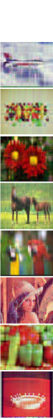
The widely used $8$ color images with different sizes are selected as the test samples shown in Fig.1. Similar to the settings in [13, 39, 24], all real matrix completion methods among the compared methods are performed on each channel of the test images individually.

Refer to caption
Figure 1: The $8$ color images (from left to right, Image(1) $256\times 256\times 3$, Image(2) $256\times 256\times 3$, Image(3) $256\times 256\times 3$, Image(4) $256\times 256\times 3$, Image(5) $256\times 256\times 3$, Image(6) $256\times 256\times 3$, Image(7) $256\times 256\times 3$ and Image (8) $256\times 256\times 3$).
Refer to caption
Refer to caption
Refer to caption
Figure 2: Relative error (RE) versus iteration on all images (from left to right: (a) Q-DFN, (b) Q-DNN and (c) Q-FNN).

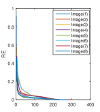
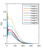
Fig.2 shows the empirical convergence of the proposed three methods for color image inpainting on all images with ${\rm{MR}}=0.50$, where ${\rm{MR}}$ denotes the missing ratio of pixels (the larger the value of ${\rm{MR}}$, the more pixels are lost).

Refer to caption
Refer to caption
Refer to caption
Refer to caption
Refer to caption
Refer to caption
Refer to caption
Refer to caption
Refer to caption
Refer to caption
Refer to caption
Images Indexes D-N [13] F-N [13] WNNM [6] MC-NC [37] LRQA-2 [24] RegL1-ALM [12] Q-DFN Q-DNN Q-FNN
Image(1) PSNR 20.956 21.313 23.549 26.002 25.767 20.467 25.332 26.085 26.170
SSIM 0.404 0.413 0.430 0.607 0.735 0.508 0.761 0.747 0.769
time(s) 25.08 20.05 142.27 93.56 743.07 636.51 94.31 129.04 137.67
Image(2) PSNR 21.067 23.259 23.648 25.604 25.679 21.777 25.291 25.901 26.017
SSIM 0.834 0.877 0.884 0.926 0.929 0.877 0.928 0.931 0.937
time(s) 5.54 5.06 41.80 28.32 92.44 154.19 60.10 66.05 73.79
Image(3) PSNR 21.383 21.350 23.554 25.121 25.764 19.367 25.672 25.985 26.007
SSIM 0.741 0.745 0.789 0.847 0.913 0.742 0.915 0.916 0.920
time(s) 18.02 14.08 89.17 281.25 407.69 368.69 64.63 99.22 121.30
Image(4) PSNR 19.722 19.774 18.945 20.013 21.665 19.423 21.780 21.686 21.636
SSIM 0.764 0.762 0.718 0.775 0.850 0.764 0.856 0.852 0.848
time(s) 17.95 14.24 87.36 216.34 337.88 498.33 77.68 109.30 126.18
Image(5) PSNR 22.804 22.847 25.899 27.453 27.795 21.212 27.721 27.969 28.040
SSIM 0.860 0.854 0.857 0.913 0.928 0.776 0.929 0.930 0.932
time(s) 31.52 27.86 264.36 160.73 1694.73 825.09 122.23 179.18 200.70
Image(6) PSNR 21.359 20.637 21.265 23.426 23.878 19.198 23.482 23.724 24.065
SSIM 0.865 0.852 0.853 0.912 0.924 0.845 0.924 0.919 0.925
time(s) 7.10 6.27 40.71 24.77 85.99 123.76 61.54 61.47 71.98
Image(7) PSNR 18.998 18.745 23.012 25.957 25.909 17.358 25.801 25.735 26.403
SSIM 0.834 0.833 0.895 0.941 0.945 0.809 0.937 0.942 0.951
time(s) 25.00 20.92 151.91 122.56 796.07 548.46 110.09 126.56 132.61
Image(8) PSNR 24.607 25.823 28.377 30.422 30.040 24.799 29.850 30.475 30.573
SSIM 0.918 0.924 0.935 0.956 0.965 0.930 0.961 0.967 0.969
time(s) 24.55 19.49 148.67 70.87 880.53 852.91 107.51 128.68 130.61
(a) Bold fonts denote the best performance; underline ones represent the second-best results.
Figure 3: (a) is the original image. (b) is the observed image (${\rm{MR}}=0.70$). (c)-(k) are the inpainting results of D-N, F-N, WNNM, MC-NC, LRQA-2, RegL1-ALM, Q-DFN, Q-DNN and Q-FNN, respectively. (l) summaries the PSNR values, SSIM values and the running time of all methods. The figure is viewed better in zoomed PDF.
Refer to caption
Figure 4: Average runtime (second) of all methods for color image inpainting on the eight testing color images with different ${\rm{MRs}}$.
TABLE IV: Quantitative assessment indexes (PSNR/SSIM) of different methods on the eight color images (Bold fonts denote the best performance; underline ones represent the second-best results).
Methods: D-N [13] F-N [13] WNNM [6] MC-NC [37] LRQA-2 [24] RegL1-ALM [12] Q-DFN Q-DNN Q-FNN
Images: ${\rm{MR}}=0.50$
Image(1) 21.409/0.421 21.409/0.422 28.388/0.605 29.154/0.778 29.171/0.829 19.324/0.483 30.055/0.885 30.702/0.878 30.526/0.883
Image(2) 22.990/0.858 22.977/0.857 29.350/0.957 30.865/0.974 30.275/0.970 20.881/0.880 30.180/0.973 30.947/0.975 30.173/0.971
Image(3) 21.833/0.742 21.833/0.742 27.630/0.901 29.674/0.944 29.556/0.964 20.084/0.789 29.408/0.968 29.724/0.967 29.591/0.966
Image(4) 21.048/0.780 21.048/0.780 21.631/0.835 23.888/0.900 24.316/0.912 19.671/0.789 24.400/0.919 24.043/0.914 24.308/0.918
Image(5) 23.670/0.801 23.670/0.802 29.858/0.921 31.562/0.957 30.645/0.952 20.897/0.771 31.539/0.967 31.838/0.966 31.798/0.967
Image(6) 21.912/0.875 21.001/0.879 24.960/0.929 27.760/0.967 27.469/0.962 19.965/0.870 27.474/0.965 27.475/0.964 27.192/0.961
Image(7) 19.636/0.842 19.638/0.844 26.805/0.950 29.247/0.972 29.277/0.972 17.317/0.816 29.151/0.972 29.541/0.973 29.836/0.976
Image(8) 25.144/0.924 25.146/0.926 32.508/0.962 34.203/0.978 33.286/0.981 22.842/0.924 34.069/0.984 34.686/0.987 34.144/0.985
Aver. 22.205 22.090 27.641 29.540 29.249 20.122 29.534 29.869 29.696
Images ${\rm{MR}}=0.75$
Image(1) 20.761/0.398 20.759/0.393 21.189/0.379 24.724/0.543 24.659/0.697 19.926/0.484 24.133/0.719 24.841/0.699 25.134/0.725
Image(2) 20.871/0.827 20.876/0.827 21.850/0.841 23.799/0.891 24.111/0.905 19.854/0.842 23.778/0.905 24.638/0.913 24.520/0.912
Image(3) 20.326/0.706 20.331/0.707 22.367/0.741 23.902/0.808 24.738/0.889 19.584/0.750 24.273/0.885 24.956/0.894 25.069/0.897
Image(4) 19.358/0.751 19.355/0.751 18.107/0.671 19.237/0.737 21.050/0.826 18.975/0.753 20.963/0.830 20.719/0.812 20.858/0.819
Image(5) 22.388/0.769 22.387/0.769 24.746/0.827 26.455/0.896 26.933/0.915 21.743/0.769 26.694/0.916 26.949/0.915 27.023/0.919
Image(6) 19.833/0.813 19.906/0.815 20.014/0.816 22.151/0.886 22.743/0.904 18.425/0.773 22.334/0.907 22.907/0.904 23.107/0.910
Image(7) 18.528/0.824 18.528/0.824 21.850/0.870 24.459/0.926 24.792/0.932 17.287/0.813 23.869/0.920 24.727/0.930 25.076/0.936
Image(8) 24.508/0.910 24.491/0.911 27.182/0.923 28.981/0.946 28.666/0.957 23.232/0.921 28.001/0.953 29.144/0.960 29.247/0.962
Aver. 20.817 20.829 22.163 24.213 24.711 19.878 24.289 24.860 25.004
Images ${\rm{MR}}=0.85$
Image(1) 19.847/0.317 19.859/0.317 18.877/0.251 20.651/0.352 21.604/0.567 18.821/0.339 21.391/0.584 21.860/0.570 22.066/0.596
Image(2) 18.979/0.740 19.073/0.747 18.277/0.739 19.285/0.776 20.924/0.832 17.533/0.691 21.120/0.853 21.154/0.844 21.601/0.860
Image(3) 20.427/0.698 20.436/0.698 19.548/0.619 20.488/0.674 22.201/0.804 19.660/0.718 21.386/0.790 22.007/0.796 22.299/0.818
Image(4) 17.578/0.655 17.605/0.658 16.295/0.570 17.353/0.633 19.316/0.766 16.211/0.615 19.412/0.776 19.226/0.749 19.507/0.766
Image(5) 21.905/0.742 21.922/0.743 22.089/0.740 23.603/0.823 24.512/0.853 21.498/0.757 24.244/0.876 24.532/0.865 24.806/0.879
Image(6) 18.287/0.755 18.169/0.750 17.218/0.709 18.297/0.769 20.334/0.855 17.157/0.708 19.662/0.853 20.471/0.859 20.444/0.860
Image(7) 19.685/0.835 19.674/0.836 18.556/0.773 20.017/0.829 21.823/0.885 19.282/0.837 20.817/0.869 21.355/0.869 22.118/0.891
Image(8) 23.628/0.897 23.683/0.898 23.636/0.885 24.857/0.909 25.863/0.935 21.815/0.876 24.842/0.928 25.933/0.937 26.189/0.939
Aver. 20.042 20.053 19.312 20.569 22.072 18.997 21.606 22.067 22.379
Refer to caption
(a) Original
Refer to caption
(b) Observed
Refer to caption
(c) D-N [13]
Refer to caption
(d) F-N [13]
Refer to caption
(e) WNNM [6]
Refer to caption
(f) MC-NC [37]
Refer to caption
(g) LRQA-2 [24]
Refer to caption
(h) RegL1-ALM [12]
Refer to caption
(i) Q-DFN
Refer to caption
(j) Q-DNN
Refer to caption
(k) Q-FNN
Figure 5: Color image inpainting results on Image(1). (a) is the original image. (b) is the observed image (${\rm{MR}}=0.75$). (c)-(k) are the inpainting results of D-N, F-N, WNNM, MC-NC, LRQA-2, RegL1-ALM, Q-DFN, Q-DNN and Q-FNN, respectively.

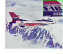
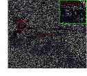
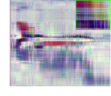
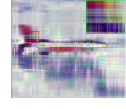
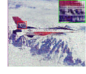
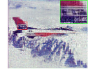
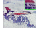
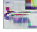
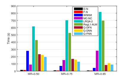
Fig.3 displays the visual and quantitative comparisons between the proposed three methods and all compared inpainting methods on the eight testing color images with ${\rm{MR}}=0.70$. TABLE IV reports the quantitative PSNR and SSIM values (and the average values of PSNR) of all inpainting methods on the eight testing color images with different ${\rm{MRs}}$. Fig.4 shows the average runtime of all methods for color image inpainting on the eight testing color images with different ${\rm{MRs}}$. From all the experimental results, we can observe and summarize the following points.

  • The proposed three algorithms are indeed convergent (see Fig.2). Although the convergence curves fluctuate at the beginning of the iteration (especially Q-DNN and Q-FNN), the three algorithms converge as the number of iterations increases.

  • Compared with LRMC-based methods, LRQMC-based methods (including our proposed three methods and LRQA-2) , in the overwhelming majority of cases, show better performance both visually (see Fig.3 and Fig.5) and quantitatively (see TABLE IV). It is mainly due to the advantage of quaternion representation of color pixel values. As the latest LRMC-based method, MC-NC shows the comparable performance with the LRQMC-based methods for lower ${\rm{MR}}$ values, e.g., ${\rm{MR}}=0.50$.

  • As LRQMC-based methods, the performance of LRQA-2, and the proposed Q-DFN, Q-DNN and Q-FNN are very close. Nonetheless, the runtime of the proposed Q-DFN, Q-DNN and Q-FNN is much shorter than that of LRQA-2 (see Fig.4). This is mainly because our proposed methods only need to handle two much smaller factor quaternion matrices rather than calculating the QSVD of original big size quaternion matrices in each iteration as LRQA-2 must do.

V Conclusion

We propose three novel low-rank quaternion matrix completion (LRQMC) methods, named Q-DFN, Q-DNN, and Q-FFN to recover missing data of the color image, which can holistically handle the three RGB channels. Based on three quaternion-based bilinear factor (QBF) matrix norm minimization models, the proposed methods only need to process two much smaller factor quaternion matrices, thus it can effectively reduce the time consumption caused by the calculation of quaternion singular value decompositions (QSVD). The alternating direction method of multipliers (ADMM) framework is applied to solve the models, which indeed guarantees the convergence (as we empirically show in the experiments ) of the proposed algorithms. Furthermore, experimental results on real color image inpainting also demonstrate the effectiveness of the developed methods.

One of our future work aims to extend the proposed models to some other low-rank quaternion matrix approximate problems such as color face recognition, color image superresolution, and color image denoising. Recently, some convolutional neural networks (CNN)-based approaches can complete images with very large missing blocks based on numerous training samples [40]. We also would like to extend our ideas to the quaternion-based convolutional neural networks (QCNN) [41] framework in the next works.

Appendix A Basic knowledge of quaternion algebras

Quaternion space $\mathbb{H}$ was first introduced by W. Hamilton [42] in 1843, which is an extension of the complex space $\mathbb{C}$. A quaternion $\dot{q}\in\mathbb{H}$ with a real component and three imaginary components is defined as

$$\footnotesize\dot{q}=q_{0}+q_{1}i+q_{2}j+q_{3}k,$$ (45)

where $q_{l}\in\mathbb{R}\>(l=0,1,2,3)$, and $i,j,k$ are imaginary number units and obey the quaternion rules that

$\displaystyle\footnotesize\left\{\begin{array}[]{lc}i^{2}=j^{2}=k^{2}=ijk=-1,\\ ij=-ji=k,jk=-kj=i,ki=-ik=j.\end{array}\right.$ (48)

$\dot{q}$ can be decomposed into a real part $\mathfrak{R}(\dot{q}):=q_{0}$ and an imaginary part $\mathfrak{I}(\dot{q}):=q_{1}i+q_{2}j+q_{3}k$ such that $\dot{q}=\mathfrak{R}(\dot{q})+\mathfrak{I}(\dot{q})$. If the real part $\mathfrak{R}(\dot{q})=0$, $\dot{q}$ is named a pure quaternion. Given two quaternions $\dot{p}$ and $\dot{q}\in\mathbb{H}$, the sum and multiplication of them are respectively

$$\footnotesize\dot{p}+\dot{q}=(p_{0}+q_{0})+(p_{1}+q_{1})i+(p_{2}+q_{2})j+(p_{3}+q_{3})k$$

and

$\displaystyle\footnotesize\dot{p}\dot{q}=$ $\displaystyle(p_{0}q_{0}-p_{1}q_{1}-p_{2}q_{2}-p_{3}q_{3})$
$\displaystyle+(p_{0}q_{1}+p_{1}q_{0}+p_{2}q_{3}-p_{3}q_{2})i$
$\displaystyle+(p_{0}q_{2}-p_{1}q_{3}+p_{2}q_{0}+p_{3}q_{1})j$
$\displaystyle+(p_{0}q_{3}+p_{1}q_{2}-p_{2}q_{1}+p_{3}q_{0})k.$

It is noticeable that the multiplication of two quaternions is not commutative so that in general $\dot{p}\dot{q}\neq\dot{q}\dot{p}$. The conjugate and the modulus of a quaternion $\dot{q}$ are, respectively, defined as follows

$\displaystyle\footnotesize\dot{q}^{\ast}$ $\displaystyle=q_{0}-q_{1}i-q_{2}j-q_{3}k,$
$\displaystyle|\dot{q}|$ $\displaystyle=\sqrt{\dot{q}\dot{q}^{\ast}}=\sqrt{q_{0}^{2}+q_{1}^{2}+q_{2}^{2}+q_{3}^{2}}.$

Analogously, a quaternion matrix $\dot{\mathbf{Q}}=(\dot{q}_{mn})\in\mathbb{H}^{M\times N}$ is written as $\dot{\mathbf{Q}}=\mathbf{Q}_{0}+\mathbf{Q}_{1}i+\mathbf{Q}_{2}j+\mathbf{Q}_{3}k$, where $\mathbf{Q}_{l}\in\mathbb{R}^{M\times N}\>(l=0,1,2,3)$, $\dot{\mathbf{Q}}$ is named a pure quaternion matrix when $\mathfrak{R}(\dot{\mathbf{Q}})=\mathbf{Q}_{0}=\mathbf{0}$. The quaternion matrix Frobenius norm is defined as $\|\dot{\mathbf{Q}}\|_{F}=\sqrt{\sum_{m=1}^{M}\sum_{n=1}^{N}|\ddot{q}_{mn}|^{2}}=\sqrt{{\rm{tr}}\{(\dot{\mathbf{Q}})^{H}\dot{\mathbf{Q}}\}}$. Using Cayley-Dickson notation [43], $\dot{\mathbf{Q}}$ can be expressed as $\dot{\mathbf{Q}}=\mathbf{Q}_{a}+\mathbf{Q}_{b}j$, where $\mathbf{Q}_{a}=\mathbf{Q}_{0}+\mathbf{Q}_{1}i\in\mathbb{C}^{M\times N}$, $\mathbf{Q}_{b}=\mathbf{Q}_{2}+\mathbf{Q}_{3}i\in\mathbb{C}^{M\times N}$. Then the quaternion matrix $\dot{\mathbf{Q}}$ can be denoted as an equivalent complex matrix

$$\footnotesize\mathbf{Q}_{c}=\left(\begin{array}[]{cc}\mathbf{Q}_{a}&\mathbf{Q}_{b}\\ -\mathbf{Q}_{b}^{\ast}&\mathbf{Q}_{a}^{\ast}\end{array}\right)\in\mathbb{C}^{2M\times 2N}.$$ (49)

Based on (49), the QSVD of quaternion matrix $\dot{\mathbf{Q}}$ can be obtained by applying the classical complex SVD algorithm to $\mathbf{Q}_{c}$. The relation between the QSVD of quaternion matrix $\dot{\mathbf{Q}}\in\mathbb{H}^{M\times N}$ and the SVD of its equivalent complex matrix $\mathbf{Q}_{c}\in\mathbb{C}^{2M\times 2N}$ ($\mathbf{Q}_{c}=\mathbf{U}\check{\mathbf{D}}\mathbf{V}^{H}$) is defined as [44]

$\displaystyle\footnotesize\left\{\begin{array}[]{lc}\mathbf{D}={\rm{row}}_{odd}({\rm{col}}_{odd}(\check{\mathbf{D}})),\\ \dot{\mathbf{U}}={\rm{col}}_{odd}(\mathbf{U}_{1})+{\rm{col}}_{odd}(-(\mathbf{U}_{2})^{\ast})j,\\ \dot{\mathbf{V}}={\rm{col}}_{odd}(\mathbf{V}_{1})+{\rm{col}}_{odd}(-(\mathbf{V}_{2})^{\ast})j,\end{array}\right.$ (53)

such that $\dot{\mathbf{Q}}=\dot{\mathbf{U}}\mathbf{D}\dot{\mathbf{V}}^{H}$, where

$\displaystyle\footnotesize\mathbf{U}=\left(\begin{array}[]{c}(\mathbf{U}_{1})_{M\times 2M}\\ (\mathbf{U}_{2})_{M\times 2M}\end{array}\right),\quad\mathbf{V}=\left(\begin{array}[]{c}(\mathbf{V}_{1})_{N\times 2N}\\ (\mathbf{V}_{2})_{N\times 2N}\end{array}\right),$

and ${\rm{row}}_{odd}(\mathbf{M})$, ${\rm{col}}_{odd}(\mathbf{M})$ respectively extract the odd rows and odd columns of matrix $\mathbf{M}$.

Readers can find more details on quaternion algebra in [28, 45, 46].

Appendix B The proof of Theorem 2

Proof: According to the QSVD in Theorem 1, there exist unitary quaternion matrices $\dot{\mathbf{A}}\in\mathbb{H}^{M\times M}$ and $\dot{\mathbf{B}}\in\mathbb{H}^{N\times N}$ such that

$$\footnotesize\dot{\mathbf{X}}=\dot{\mathbf{A}}\left(\begin{array}[]{cc}\mathbf{D}_{d}&\mathbf{0}\\ \mathbf{0}&\mathbf{0}\end{array}\right)\dot{\mathbf{B}}^{H},$$ (54)

where $\mathbf{D}_{d}={\rm{diag}}\{d_{1},\ldots,d_{r},d_{r+1},\ldots,d_{d}\}\in\mathbb{R}^{d\times d}$ and the $d_{1},\ldots,d_{r}$ are the positive singular values of $\dot{\mathbf{X}}$, $d_{r+1},\ldots,d_{d}$ are equal to 00. Then, (54) can be rewritten as

$$\footnotesize\dot{\mathbf{X}}=\dot{\mathbf{A}}\left(\begin{array}[]{c}\mathbf{D}_{d}^{\frac{1}{2}}\\ \mathbf{0}\end{array}\right)_{M\times d}\left(\begin{array}[]{cc}\mathbf{D}_{d}^{\frac{1}{2}}&\mathbf{0}\end{array}\right)_{d\times N}\dot{\mathbf{B}}^{H}.$$

Let $\dot{\mathbf{U}}=\dot{\mathbf{A}}\left(\begin{array}[]{c}\mathbf{D}_{d}^{\frac{1}{2}}\\ \mathbf{0}\end{array}\right)\in\mathbb{H}^{M\times d}$ and $\dot{\mathbf{V}}=\dot{\mathbf{B}}\left(\begin{array}[]{c}\mathbf{D}_{d}^{\frac{1}{2}}\\ \mathbf{0}\end{array}\right)\in\mathbb{H}^{N\times d}$, they obviously meet ${\rm{rank}}(\dot{\mathbf{U}})={\rm{rank}}(\dot{\mathbf{V}})=r$, and $\dot{\mathbf{X}}=\dot{\mathbf{U}}\dot{\mathbf{V}}^{H}$.

Appendix C The proofs of Theorem 3, Theorem 4 and Theorem 5

To prove the Theorem 3, Theorem 4 and Theorem 5, we first give the following lemma.

Lemma 1.

Let two quaternion matrices $\dot{\mathbf{U}}\in\mathbb{H}^{M\times d}$ and $\dot{\mathbf{V}}\in\mathbb{H}^{N\times d}$ be given and let $p>0$, denote $K={\rm{min}}(M,N,d)$, the following inequality holds for the decreasingly ordered singular values of $\dot{\mathbf{U}}\dot{\mathbf{V}}^{H}$, $\dot{\mathbf{U}}$ and $\dot{\mathbf{V}}$.

$$\footnotesize\sum_{k}^{K}\sigma_{k}^{p}(\dot{\mathbf{U}}\dot{\mathbf{V}}^{H})\leq\sum_{k}^{K}\sigma_{k}^{p}(\dot{\mathbf{U}})\sigma_{k}^{p}(\dot{\mathbf{V}}).$$ (55)

Proof:

$\displaystyle\footnotesize\sum_{k}^{K}\sigma_{k}^{p}(\dot{\mathbf{U}}\dot{\mathbf{V}}^{H})$ $\displaystyle=\frac{1}{2}\sum_{k}^{K}\sigma_{k}^{p}(\mathcal{P}(\dot{\mathbf{U}}\dot{\mathbf{V}}^{H}))$
$\displaystyle=\frac{1}{2}\sum_{k}^{K}\sigma_{k}^{p}(\mathcal{P}(\dot{\mathbf{U}})\mathcal{P}(\dot{\mathbf{V}}^{H}))$
$\displaystyle\leq\frac{1}{2}\sum_{k}^{K}\sigma_{k}^{p}(\mathcal{P}(\dot{\mathbf{U}}))\sigma_{k}^{p}(\mathcal{P}(\dot{\mathbf{V}}^{H}))$
$\displaystyle=\sum_{k}^{K}\sigma_{k}^{p}(\dot{\mathbf{U}})\sigma_{k}^{p}(\dot{\mathbf{V}}),$

where the inequality follows from [47] (Theorem 3.3.14).

Proof of Theorem 3: Since $\dot{\mathbf{X}}=\dot{\mathbf{U}}\dot{\mathbf{V}}^{H}$, where $\dot{\mathbf{U}}\in\mathbb{H}^{M\times d}$ and $\dot{\mathbf{V}}\in\mathbb{H}^{N\times d}$, denote $K={\rm{min}}(M,N,d)$, we have

$\displaystyle\footnotesize\|\dot{\mathbf{X}}\|_{\ast}$ $\displaystyle=\sum_{k}^{K}\sigma_{k}(\dot{\mathbf{X}})=\sum_{k}^{K}\sigma_{k}(\dot{\mathbf{U}}\dot{\mathbf{V}}^{H})\leq\sum_{k}^{K}\sigma_{k}(\dot{\mathbf{U}})\sigma_{k}(\dot{\mathbf{V}})$
$\displaystyle\leq\left(\sum_{k}^{K}\sigma_{k}^{2}(\dot{\mathbf{U}})\right)^{1/2}\left(\sum_{k}^{K}\sigma_{k}^{2}(\dot{\mathbf{V}})\right)^{1/2}$
$\displaystyle\leq\frac{1}{2}\left(\sum_{k}^{K}\sigma_{k}^{2}(\dot{\mathbf{U}})\right)+\frac{1}{2}\left(\sum_{k}^{K}\sigma_{k}^{2}(\dot{\mathbf{V}})\right)$
$\displaystyle\leq\frac{1}{2}\left(\sum_{k}^{{\rm{min}}(M,d)}\!\!\!\!\sigma_{k}^{2}(\dot{\mathbf{U}})\right)+\frac{1}{2}\left(\sum_{k}^{{\rm{min}}(N,d)}\!\!\!\!\sigma_{k}^{2}(\dot{\mathbf{V}})\right)$
$\displaystyle=\frac{1}{2}\left(\|\dot{\mathbf{U}}\|_{F}^{2}+\|\dot{\mathbf{V}}\|_{F}^{2}\right),$

where the first inequality follows from Lemma 1 as $p=1$, the second inequality follows from the well-known Holder’s inequality [48], the third inequality holds due to the Jensen’s inequality [49], and since we always have $K={\rm{min}}(M,N,d)\leq{\rm{min}}(M,d),K={\rm{min}}(M,N,d)\leq{\rm{min}}(N,d)$, thus the last inequality holds. On the other hand, let $\dot{\mathbf{U}}_{\star}=\dot{\mathbf{A}}_{\dot{\mathbf{X}}}\mathbf{D}_{\dot{\mathbf{X}}}^{\frac{1}{2}}$ and $\dot{\mathbf{V}}_{\star}=\dot{\mathbf{B}}_{\dot{\mathbf{X}}}\mathbf{D}_{\dot{\mathbf{X}}}^{\frac{1}{2}}$, where $\dot{\mathbf{X}}=\dot{\mathbf{A}}_{\dot{\mathbf{X}}}\mathbf{D}_{\dot{\mathbf{X}}}\dot{\mathbf{B}}_{\dot{\mathbf{X}}}^{H}$ is the QSVD of $\dot{\mathbf{X}}$. Then, we have $\dot{\mathbf{X}}=\dot{\mathbf{U}}_{\star}\dot{\mathbf{V}}_{\star}^{H}$ and $\|\dot{\mathbf{X}}\|_{\ast}=\frac{1}{2}\left(\|\dot{\mathbf{U}}_{\star}\|_{F}^{2}+\|\dot{\mathbf{V}}_{\star}\|_{F}^{2}\right)$.

Hence, from above, we have

$$\footnotesize\mathop{{\rm{min}}}\limits_{\dot{\mathbf{U}},\dot{\mathbf{V}}\atop\dot{\mathbf{X}}=\dot{\mathbf{U}}\dot{\mathbf{V}}^{H}}\frac{1}{2}\|\dot{\mathbf{U}}\|_{F}^{2}+\frac{1}{2}\|\dot{\mathbf{V}}\|_{F}^{2}=\|\dot{\mathbf{X}}\|_{\ast}.$$

Proof of Theorem 4: Since $\dot{\mathbf{X}}=\dot{\mathbf{U}}\dot{\mathbf{V}}^{H}$, where $\dot{\mathbf{U}}\in\mathbb{H}^{M\times d}$ and $\dot{\mathbf{V}}\in\mathbb{H}^{N\times d}$, denote $K={\rm{min}}(M,N,d)$, we have

$\displaystyle\footnotesize\|\dot{\mathbf{X}}\|_{Q-S_{1/2}}^{1/2}$ $\displaystyle=\sum_{k}^{K}\sigma_{k}^{1/2}(\dot{\mathbf{X}})=\sum_{k}^{K}\sigma_{k}^{1/2}(\dot{\mathbf{U}}\dot{\mathbf{V}}^{H})$
$\displaystyle\leq\sum_{k}^{K}\sigma_{k}^{1/2}(\dot{\mathbf{U}})\sigma_{k}^{1/2}(\dot{\mathbf{V}})$
$\displaystyle\leq\left(\sum_{k}^{K}\sigma_{k}(\dot{\mathbf{U}})\right)^{1/2}\left(\sum_{k}^{K}\sigma_{k}(\dot{\mathbf{V}})\right)^{1/2}$
$\displaystyle\leq\frac{1}{2}\left(\sum_{k}^{K}\sigma_{k}(\dot{\mathbf{U}})\right)+\frac{1}{2}\left(\sum_{k}^{K}\sigma_{k}(\dot{\mathbf{V}})\right)$
$\displaystyle\leq\frac{1}{2}\left(\sum_{k}^{{\rm{min}}(M,d)}\!\!\!\!\sigma_{k}(\dot{\mathbf{U}})\!\right)+\frac{1}{2}\left(\sum_{k}^{{\rm{min}}(N,d)}\!\!\!\!\sigma_{k}(\dot{\mathbf{V}})\!\right)$
$\displaystyle=\frac{1}{2}\left(\|\dot{\mathbf{U}}\|_{\ast}+\|\dot{\mathbf{V}}\|_{\ast}\right),$

where the first inequality follows from Lemma 1 as $p=\frac{1}{2}$, the second inequality follows from the well-known Holder’s inequality [48], the third inequality holds due to the Jensen’s inequality [49], and since we always have $K={\rm{min}}(M,N,d)\leq{\rm{min}}(M,d),K={\rm{min}}(M,N,d)\leq{\rm{min}}(N,d)$, thus the last inequality holds. On the other hand, let $\dot{\mathbf{U}}_{\star}=\dot{\mathbf{A}}_{\dot{\mathbf{X}}}\mathbf{D}_{\dot{\mathbf{X}}}^{\frac{1}{2}}$ and $\dot{\mathbf{V}}_{\star}=\dot{\mathbf{B}}_{\dot{\mathbf{X}}}\mathbf{D}_{\dot{\mathbf{X}}}^{\frac{1}{2}}$, where $\dot{\mathbf{X}}=\dot{\mathbf{A}}_{\dot{\mathbf{X}}}\mathbf{D}_{\dot{\mathbf{X}}}\dot{\mathbf{B}}_{\dot{\mathbf{X}}}^{H}$ is the QSVD of $\dot{\mathbf{X}}$. Then, we have $\dot{\mathbf{X}}=\dot{\mathbf{U}}_{\star}\dot{\mathbf{V}}_{\star}^{H}$ and $\|\dot{\mathbf{X}}\|_{Q-S_{1/2}}=\frac{1}{4}\left(\|\dot{\mathbf{U}}_{\star}\|_{\ast}+\|\dot{\mathbf{V}}_{\star}\|_{\ast}\right)^{2}$.

Hence, from above, we have

$$\footnotesize\mathop{{\rm{min}}}\limits_{\dot{\mathbf{U}},\dot{\mathbf{V}}\atop\dot{\mathbf{X}}=\dot{\mathbf{U}}\dot{\mathbf{V}}^{H}}\frac{1}{4}\left(\|\dot{\mathbf{U}}\|_{\ast}+\|\dot{\mathbf{V}}\|_{\ast}\right)^{2}=\|\dot{\mathbf{X}}\|_{Q-S_{1/2}}.$$

Proof of Theorem 5: Since $\dot{\mathbf{X}}=\dot{\mathbf{U}}\dot{\mathbf{V}}^{H}$, where $\dot{\mathbf{U}}\in\mathbb{H}^{M\times d}$ and $\dot{\mathbf{V}}\in\mathbb{H}^{N\times d}$, denote $K={\rm{min}}(M,N,d)$, we have

$\displaystyle\footnotesize\|\dot{\mathbf{X}}\|_{Q-S_{2/3}}^{2/3}$ $\displaystyle=\sum_{k}^{K}\sigma_{k}^{2/3}(\dot{\mathbf{X}})=\sum_{k}^{K}\sigma_{k}^{2/3}(\dot{\mathbf{U}}\dot{\mathbf{V}}^{H})$
$\displaystyle\leq\sum_{k}^{K}\sigma_{k}^{2/3}(\dot{\mathbf{U}})\sigma_{k}^{2/3}(\dot{\mathbf{V}})$
$\displaystyle\leq\left(\sum_{k}^{K}\sigma_{k}^{\frac{2}{3}*3}(\dot{\mathbf{U}})\right)^{1/3}\left(\sum_{k}^{K}\sigma_{k}^{\frac{2}{3}*\frac{3}{2}}(\dot{\mathbf{V}})\right)^{2/3}$
$\displaystyle\leq\frac{1}{3}\left(\sum_{k}^{K}\sigma_{k}^{2}(\dot{\mathbf{U}})\right)+\frac{2}{3}\left(\sum_{k}^{K}\sigma_{k}(\dot{\mathbf{V}})\right)$
$\displaystyle\leq\frac{1}{3}\left(\sum_{k}^{{\rm{min}}(M,d)}\!\!\!\!\sigma_{k}^{2}(\dot{\mathbf{U}})\right)+\frac{2}{3}\left(\sum_{k}^{{\rm{min}}(N,d)}\!\!\!\!\sigma_{k}(\dot{\mathbf{V}})\right)$
$\displaystyle=\frac{1}{3}\left(\|\dot{\mathbf{U}}\|_{F}^{2}+2\|\dot{\mathbf{V}}\|_{\ast}\right),$

where the first inequality follows from Lemma 1 as $p=\frac{2}{3}$, the second inequality follows from the well-known Holder’s inequality [48], the third inequality holds due to the Jensen’s inequality [49], and since we always have $K={\rm{min}}(M,N,d)\leq{\rm{min}}(M,d),K={\rm{min}}(M,N,d)\leq{\rm{min}}(N,d)$, thus the last inequality holds. On the other hand, let $\dot{\mathbf{U}}_{\star}=\dot{\mathbf{A}}_{\dot{\mathbf{X}}}\mathbf{D}_{\dot{\mathbf{X}}}^{\frac{1}{3}}$ and $\dot{\mathbf{V}}_{\star}=\dot{\mathbf{B}}_{\dot{\mathbf{X}}}\mathbf{D}_{\dot{\mathbf{X}}}^{\frac{2}{3}}$, where $\dot{\mathbf{X}}=\dot{\mathbf{A}}_{\dot{\mathbf{X}}}\mathbf{D}_{\dot{\mathbf{X}}}\dot{\mathbf{B}}_{\dot{\mathbf{X}}}^{H}$ is the QSVD of $\dot{\mathbf{X}}$. Then, we have $\dot{\mathbf{X}}=\dot{\mathbf{U}}_{\star}\dot{\mathbf{V}}_{\star}^{H}$ and $\|\dot{\mathbf{X}}\|_{Q-S_{2/3}}=\left((\|\dot{\mathbf{U}}_{\star}\|_{F}^{2}+2\|\dot{\mathbf{V}}_{\star}\|_{\ast})/3\right)^{3/2}$.

Hence, from above, we have

$$\footnotesize\mathop{{\rm{min}}}\limits_{\dot{\mathbf{U}},\dot{\mathbf{V}}\atop\dot{\mathbf{X}}=\dot{\mathbf{U}}\dot{\mathbf{V}}^{H}}\left(\frac{\|\dot{\mathbf{U}}\|_{F}^{2}+2\|\dot{\mathbf{V}}\|_{\ast}}{3}\right)^{3/2}=\|\dot{\mathbf{X}}\|_{Q-S_{2/3}}.$$

Appendix D Solving the problem (29)

Similar to the problem (28), the problem (29) is solved by minimizing the following augmented Lagrangian function

$$\footnotesize\begin{split}&\mathcal{L}_{\mu}(\dot{\mathbf{U}},\dot{\mathbf{V}},\dot{\mathbf{A}}_{V},\dot{\mathbf{X}},\dot{\mathbf{F}}_{1},\dot{\mathbf{F}}_{2})\\ &=\frac{\lambda}{3}\big{(}\|\dot{\mathbf{U}}\|_{F}^{2}+2\|\dot{\mathbf{A}}_{V}\|_{\ast}\big{)}+\langle\dot{\mathbf{F}}_{1},\dot{\mathbf{V}}-\dot{\mathbf{A}}_{V}\rangle\\ &\quad+\langle\dot{\mathbf{F}}_{2},\dot{\mathbf{X}}-\dot{\mathbf{U}}\dot{\mathbf{V}}^{H}\rangle+\frac{\mu}{2}\left(\|\dot{\mathbf{V}}-\dot{\mathbf{A}}_{V}\|_{F}^{2}\right.\\ &\quad\left.+\|\dot{\mathbf{X}}-\dot{\mathbf{U}}\dot{\mathbf{V}}^{H}\|_{F}^{2}\right)+\frac{1}{2}\|\mathcal{P}_{\Omega}(\dot{\mathbf{X}}-\dot{\mathbf{T}})\|_{F}^{2},\end{split}$$ (56)

where $\mu>0$ is the penalty parameter, $\dot{\mathbf{F}}_{1}$ and $\dot{\mathbf{F}}_{2}$ are Lagrange multipliers.

Updating $\dot{\mathbf{U}}$ and $\dot{\mathbf{V}}$:

$$\footnotesize\begin{split}\dot{\mathbf{U}}^{\tau+1}=&\mathop{{\rm{arg\,min}}}\limits_{\dot{\mathbf{U}}}\ \frac{1}{2}\|\dot{\mathbf{X}}^{\tau}-\dot{\mathbf{U}}(\dot{\mathbf{V}}^{\tau})^{H}+\dot{\mathbf{F}}_{2}^{\tau}/\mu^{\tau}\|_{F}^{2}\\ &+\frac{\lambda}{3\mu^{\tau}}\|\dot{\mathbf{U}}\|_{F}^{2}\end{split}$$ (57)
$$\footnotesize\begin{split}\dot{\mathbf{V}}^{\tau+1}=&\mathop{{\rm{arg\,min}}}\limits_{\dot{\mathbf{V}}}\ \|\dot{\mathbf{V}}-\dot{\mathbf{A}}_{V}^{\tau}+\dot{\mathbf{F}}_{1}^{\tau}/\mu^{\tau}\|_{F}^{2}\\ &+\|\dot{\mathbf{X}}^{\tau}-\dot{\mathbf{U}}^{\tau+1}\dot{\mathbf{V}}^{H}+\dot{\mathbf{F}}_{2}^{\tau}/\mu^{\tau}\|_{F}^{2}.\end{split}$$ (58)

By the similar way as (33), we can obtain the optimal solution of $\dot{\mathbf{U}}^{\tau+1}$ and $\dot{\mathbf{V}}^{\tau+1}$ as

$$\footnotesize\dot{\mathbf{U}}^{\tau+1}=\left((\mu^{\tau}\dot{\mathbf{X}}^{\tau}+\dot{\mathbf{F}}_{2}^{\tau})\dot{\mathbf{V}}^{\tau}\right)\left(\frac{2\lambda}{3}\mathbf{I}+\mu^{\tau}(\dot{\mathbf{V}}^{\tau})^{H}\dot{\mathbf{V}}^{\tau}\right)^{-1}.$$ (59)
$$\footnotesize\begin{split}\dot{\mathbf{V}}^{\tau+1}=&\left(\dot{\mathbf{A}}_{V}^{\tau}-\dot{\mathbf{F}}_{1}^{\tau}/\mu^{\tau}+(\dot{\mathbf{X}}^{\tau}\right.\\ &\left.+\dot{\mathbf{F}}_{2}^{\tau}/\mu^{\tau})^{H}\dot{\mathbf{U}}^{\tau+1}\right)\left(\mathbf{I}+(\dot{\mathbf{U}}^{\tau+1})^{H}\dot{\mathbf{U}}^{\tau+1}\right)^{-1}.\\ \end{split}$$ (60)

Updating $\dot{\mathbf{A}}_{V}$:

$$\footnotesize\begin{split}\dot{\mathbf{A}}_{V}^{\tau+1}=&\mathop{{\rm{arg\,min}}}\limits_{\dot{\mathbf{A}}_{V}}\ \frac{1}{2}\|\dot{\mathbf{A}}_{V}-(\dot{\mathbf{V}}^{\tau+1}+\dot{\mathbf{F}}_{1}^{\tau}/\mu^{\tau})\|_{F}^{2}\\ &+\frac{2\lambda}{3\mu^{\tau}}\|\dot{\mathbf{A}}_{V}\|_{\ast}.\end{split}$$ (61)

The closed-form solution of (61) can be obtained by the QSVT i.e.,

$$\footnotesize\dot{\mathbf{A}}_{V}^{\tau+1}=\mathcal{D}_{\frac{2\lambda}{3\mu^{\tau}}}\left(\dot{\mathbf{V}}^{\tau+1}+\dot{\mathbf{F}}_{1}^{\tau}/\mu^{\tau}\right).$$ (62)

Updating $\dot{\mathbf{X}}$:

$$\footnotesize\begin{split}\dot{\mathbf{X}}^{\tau+1}=&\mathop{{\rm{arg\,min}}}\limits_{\dot{\mathbf{X}}}\ \frac{1}{2}\|\mathcal{P}_{\Omega}(\dot{\mathbf{X}}-\dot{\mathbf{T}})\|_{F}^{2}\\ &+\frac{\mu^{\tau}}{2}\|\dot{\mathbf{X}}-\big{(}\dot{\mathbf{U}}^{\tau+1}(\dot{\mathbf{V}}^{\tau+1})^{H}-\frac{\dot{\mathbf{F}}_{2}^{\tau}}{\mu^{\tau}}\big{)}\|_{F}^{2}.\end{split}$$ (63)

Then, we can directly obtain the optimal $\dot{\mathbf{X}}^{\tau+1}$ as

$$\footnotesize\begin{split}\dot{\mathbf{X}}^{\tau+1}=&\mathcal{P}_{\Omega^{c}}\big{(}\dot{\mathbf{U}}^{\tau+1}(\dot{\mathbf{V}}^{\tau+1})^{H}-\dot{\mathbf{F}}_{2}^{\tau}/\mu^{\tau}\big{)}\\ &+\mathcal{P}_{\Omega}\bigg{(}\frac{\mu^{\tau}\dot{\mathbf{U}}^{\tau+1}(\dot{\mathbf{V}}^{\tau+1})^{H}-\dot{\mathbf{F}}_{2}^{\tau}+\dot{\mathbf{T}}}{1+\mu^{\tau}}\bigg{)},\end{split}$$ (64)

where $\Omega^{c}$ is the complement of $\Omega$, and we have used the fact that $\mathcal{P}_{\Omega^{c}}(\dot{\mathbf{T}})=\mathbf{0}$ in (64).

Updating $\dot{\mathbf{F}}_{1},\dot{\mathbf{F}}_{2}$ and $\mu$ :

$$\footnotesize\begin{split}\dot{\mathbf{F}}_{1}^{\tau+1}&=\dot{\mathbf{F}}_{1}^{\tau}+\mu^{\tau}(\dot{\mathbf{V}}^{\tau+1}-\dot{\mathbf{A}}_{V}^{\tau+1}),\\ \dot{\mathbf{F}}_{2}^{\tau+1}&=\dot{\mathbf{F}}_{2}^{\tau}+\mu^{\tau}(\dot{\mathbf{X}}^{\tau+1}-\dot{\mathbf{U}}^{\tau+1}(\dot{\mathbf{V}}^{\tau+1})^{H}),\\ \mu^{\tau+1}&={\rm{min}}(\beta\mu^{\tau},\mu_{max}).\end{split}$$ (65)

Acknowledgment

This work was supported by The Science and Technology Development Fund, Macau SAR (File no. FDCT/085/2018/A2) and University of Macau (File no. MYRG2019-00039-FST).

References

  • [1] X. Zhou, C. Yang, H. Zhao, and W. Yu, “Low-rank modeling and its applications in image analysis,” ACM Comput. Surv., vol. 47, no. 2, pp. 36:1–36:33, 2014.
  • [2] E. J. Candès, X. Li, Y. Ma, and J. Wright, “Robust principal component analysis?” J. ACM, vol. 58, no. 3, pp. 11:1–11:37, 2011.
  • [3] J. Cai, E. J. Candès, and Z. Shen, “A singular value thresholding algorithm for matrix completion,” SIAM Journal on Optimization, vol. 20, no. 4, pp. 1956–1982, 2010.
  • [4] E. J. Candès and B. Recht, “Exact matrix completion via convex optimization,” Foundations of Computational Mathematics, vol. 9, no. 6, pp. 717–772, 2009.
  • [5] S. Gu, L. Zhang, W. Zuo, and X. Feng, “Weighted nuclear norm minimization with application to image denoising,” in 2014 IEEE Conference on Computer Vision and Pattern Recognition, CVPR 2014, Columbus, OH, USA, June 23-28, 2014, 2014, pp. 2862–2869.
  • [6] S. Gu, Q. Xie, D. Meng, W. Zuo, X. Feng, and L. Zhang, “Weighted nuclear norm minimization and its applications to low level vision,” Int. J. Comput. Vis., vol. 121, no. 2, pp. 183–208, 2017.
  • [7] F. Nie, H. Huang, and C. H. Q. Ding, “Low-rank matrix recovery via efficient schatten p-norm minimization,” in Proceedings of the Twenty-Sixth AAAI Conference on Artificial Intelligence, July 22-26, 2012, Toronto, Ontario, Canada, 2012.
  • [8] L. Liu, W. Huang, and D. Chen, “Exact minimum rank approximation via schatten p-norm minimization,” J. Comput. Appl. Math., vol. 267, pp. 218–227, 2014.
  • [9] Y. Xie, S. Gu, Y. Liu, W. Zuo, W. Zhang, and L. Zhang, “Weighted schatten p-norm minimization for image denoising and background subtraction,” IEEE Trans. Image Processing, vol. 25, no. 10, pp. 4842–4857, 2016.
  • [10] Z. Wen, W. Yin, and Y. Zhang, “Solving a low-rank factorization model for matrix completion by a nonlinear successive over-relaxation algorithm,” Math. Program. Comput., vol. 4, no. 4, pp. 333–361, 2012.
  • [11] E. Kim, M. Lee, and S. Oh, “Elastic-net regularization of singular values for robust subspace learning,” in IEEE Conference on Computer Vision and Pattern Recognition, CVPR 2015, Boston, MA, USA, June 7-12, 2015, 2015, pp. 915–923.
  • [12] Y. Zheng, G. Liu, S. Sugimoto, S. Yan, and M. Okutomi, “Practical low-rank matrix approximation under robust l1-norm,” in 2012 IEEE Conference on Computer Vision and Pattern Recognition, Providence, RI, USA, June 16-21, 2012, 2012, pp. 1410–1417.
  • [13] F. Shang, J. Cheng, Y. Liu, Z. Luo, and Z. Lin, “Bilinear factor matrix norm minimization for robust PCA: algorithms and applications,” IEEE Trans. Pattern Anal. Mach. Intell., vol. 40, no. 9, pp. 2066–2080, 2018.
  • [14] R. S. Cabral, F. D. la Torre, J. P. Costeira, and A. Bernardino, “Unifying nuclear norm and bilinear factorization approaches for low-rank matrix decomposition,” in IEEE International Conference on Computer Vision, ICCV 2013, Sydney, Australia, December 1-8, 2013, 2013, pp. 2488–2495.
  • [15] H. Fan, J. Li, Q. Yuan, X. Liu, and M. Ng, “Hyperspectral image denoising with bilinear low rank matrix factorization,” Signal Process., vol. 163, pp. 132–152, 2019.
  • [16] J. Mairal, M. Elad, and G. Sapiro, “Sparse representation for color image restoration,” IEEE Trans. Image Processing, vol. 17, no. 1, pp. 53–69, 2008.
  • [17] J. Xu, L. Zhang, D. Zhang, and X. Feng, “Multi-channel weighted nuclear norm minimization for real color image denoising,” in IEEE International Conference on Computer Vision, ICCV 2017, Venice, Italy, October 22-29, 2017, 2017, pp. 1105–1113.
  • [18] B. Chen, Q. Liu, X. Sun, X. Li, and H. Shu, “Removing gaussian noise for colour images by quaternion representation and optimisation of weights in non-local means filter,” IET Image Processing, vol. 8, no. 10, pp. 591–600, 2014.
  • [19] J. Xu, L. Ye, and W. Luo, “Color edge detection using multiscale quaternion convolution,” Int. J. Imaging Systems and Technology, vol. 20, no. 4, pp. 354–358, 2010.
  • [20] S. Gai, G. Yang, M. Wan, and L. Wang, “Denoising color images by reduced quaternion matrix singular value decomposition,” Multidim. Syst. Sign. Process., vol. 26, no. 1, pp. 307–320, 2015.
  • [21] Y. Yu, Y. Zhang, and S. Yuan, “Quaternion-based weighted nuclear norm minimization for color image denoising,” Neurocomputing, vol. 332, pp. 283–297, 2019.
  • [22] P. Bas, N. Le Bihan, and J. . Chassery, “Color image watermarking using quaternion fourier transform,” in 2003 IEEE International Conference on Acoustics, Speech, and Signal Processing, 2003. Proceedings. (ICASSP ’03)., vol. 3, April 2003, pp. III–521.
  • [23] C. Zou, K. I. Kou, and Y. Wang, “Quaternion collaborative and sparse representation with application to color face recognition,” IEEE Trans. Image Processing, vol. 25, no. 7, pp. 3287–3302, 2016.
  • [24] Y. Chen, X. Xiao, and Y. Zhou, “Low-rank quaternion approximation for color image processing,” IEEE Trans. Image Processing, vol. 29, pp. 1426–1439, 2020.
  • [25] Ö. N. Subakan and B. C. Vemuri, “A quaternion framework for color image smoothing and segmentation,” International Journal of Computer Vision, vol. 91, no. 3, pp. 233–250, 2011.
  • [26] B. Chen, H. Shu, H. Zhang, G. Chen, C. Toumoulin, J. Dillenseger, and L. Luo, “Quaternion zernike moments and their invariants for color image analysis and object recognition,” Signal Processing, vol. 92, no. 2, pp. 308–318, 2012.
  • [27] J. L. Contreras-Hernandez, D. L. Almanza-Ojeda, S. Ledesma-Orozco, A. Garcia-Perez, R. J. Romero-Troncoso, and M. A. Ibarra-Manzano, “Quaternion signal analysis algorithm for induction motor fault detection,” IEEE Transactions on Industrial Electronics, vol. 66, no. 11, pp. 8843–8850, 2019.
  • [28] F. ZHANG, “Quaternions and matrices of quaternions,” Linear akgebra abd its applications, vol. 251, pp. 21–57, 1997. [Online]. Available: https://ci.nii.ac.jp/naid/10029950538/en/
  • [29] E. J. Candès and B. Recht, “Exact matrix completion via convex optimization,” Foundations of Computational Mathematics, vol. 9, no. 6, p. 717, 2009.
  • [30] N. Gillis and F. Glineur, “Low-rank matrix approximation with weights or missing data is np-hard,” SIAM J. Matrix Analysis Applications, vol. 32, no. 4, pp. 1149–1165, 2011.
  • [31] Y. Hu, D. Zhang, J. Ye, X. Li, and X. He, “Fast and accurate matrix completion via truncated nuclear norm regularization,” IEEE Trans. Pattern Anal. Mach. Intell., vol. 35, no. 9, pp. 2117–2130, 2013.
  • [32] C. Lu, J. Tang, S. Yan, and Z. Lin, “Generalized nonconvex nonsmooth low-rank minimization,” in 2014 IEEE Conference on Computer Vision and Pattern Recognition, CVPR 2014, Columbus, OH, USA, June 23-28, 2014, 2014, pp. 4130–4137.
  • [33] M. Zhang, Z. Huang, and Y. Zhang, “Restricted p-isometry properties of nonconvex matrix recovery,” IEEE Trans. Inf. Theory, vol. 59, no. 7, pp. 4316–4323, 2013.
  • [34] H. Zhang, J. Qian, B. Zhang, J. Yang, C. Gong, and Y. Wei, “Low-rank matrix recovery via modified schatten-p norm minimization with convergence guarantees,” IEEE Trans. Image Processing, vol. 29, pp. 3132–3142, 2020.
  • [35] D. Xu and D. P. Mandic, “The theory of quaternion matrix derivatives,” IEEE Trans. Signal Processing, vol. 63, no. 6, pp. 1543–1556, 2015.
  • [36] Y. Shen, Z. Wen, and Y. Zhang, “Augmented lagrangian alternating direction method for matrix separation based on low-rank factorization,” Optimization Methods and Software, vol. 29, no. 2, pp. 239–263, 2014.
  • [37] F. Nie, Z. Hu, and X. Li, “Matrix completion based on non-convex low-rank approximation,” IEEE Trans. Image Processing, vol. 28, no. 5, pp. 2378–2388, 2019.
  • [38] Z. Wang, A. C. Bovik, H. R. Sheikh, and E. P. Simoncelli, “Image quality assessment: from error visibility to structural similarity,” IEEE Trans. Image Processing, vol. 13, no. 4, pp. 600–612, 2004.
  • [39] Y. Chen, Y. Guo, Y. Wang, D. Wang, C. Peng, and G. He, “Denoising of hyperspectral images using nonconvex low rank matrix approximation,” IEEE Trans. Geoscience and Remote Sensing, vol. 55, no. 9, pp. 5366–5380, 2017.
  • [40] C. W. Tseng, H. Lin, and S. Lai, “General deep image completion with lightweight conditional generative adversarial networks,” in British Machine Vision Conference 2017, BMVC 2017, London, UK, September 4-7, 2017, 2017.
  • [41] X. Zhu, Y. Xu, H. Xu, and C. Chen, “Quaternion convolutional neural networks,” in Computer Vision - ECCV 2018 - 15th European Conference, Munich, Germany, September 8-14, 2018, Proceedings, Part VIII, 2018, pp. 645–661.
  • [42] W. Rowan Hamilton, “Ii. on quaternions; or on a new system of imaginaries in algebra,” Phil. Mag., 3rd Ser., vol. 25, 01 1844.
  • [43] N. L. Bihan and J. I. Mars, “Singular value decomposition of quaternion matrices: a new tool for vector-sensor signal processing,” Signal Processing, vol. 84, no. 7, pp. 1177–1199, 2004.
  • [44] Y. Xu, L. Yu, H. Xu, H. Zhang, and T. Nguyen, “Vector sparse representation of color image using quaternion matrix analysis,” IEEE Trans. Image Processing, vol. 24, no. 4, pp. 1315–1329, 2015.
  • [45] P. R. Girard, Quaternions, Clifford Algebras and Relativistic Physics, 2007.
  • [46] S. L. Altmann, “Rotations, quaternions, and double groups,” Acta Crystallographica, vol. 44, no. 4, 1986.
  • [47] R. A. Horn and C. R. Johnson, Topics in Matrix Analysis.   Cambridge University Press, 1991.
  • [48] X. Yang, “Hölder’s inequality,” Appl. Math. Lett., vol. 16, no. 6, pp. 897–903, 2003.
  • [49] T. Needham, “A visual explanation of jensen’s inequality,” American Mathematical Monthly, 1993.