Transport and hydrodynamics in the chiral limit

Abstract

We analyze the evolution of hydrodynamic fluctuations for QCD matter below $T_{c}$ in the chiral limit, where the pions (the Goldstone modes) must be treated as additional non-abelian superfluid degrees of freedom, reflecting the broken $SU_{L}(2)\times SU_{R}(2)$ symmetry of the theory. In the presence of a finite pion mass $m_{\pi}$, the hydrodynamic theory is ordinary hydrodynamics at long distances, and superfluid-like at short distances. The presence of the superfluid degrees of freedom then gives specific contributions to the bulk viscosity, the shear viscosity, and diffusion coefficients of the ordinary theory at long distances which we compute. This determines, in some cases, the leading dependence of the transport parameters of QCD on the pion mass. We analyze the predictions of this computation, as the system approaches the $O(4)$ critical point.

I Introduction

Viscous hydrodynamics, based on the conservation of energy and momentum, is remarkably successful at describing a wide range of correlations observed in heavy ion collisions and has become a kind of “standard model” for heavy ion events Teaney (2010); Romatschke and Romatschke (2019). Hydrodynamics is a long wavelength effective theory which captures the underlying symmetries of the microscopic theory. In QCD this symmetry is approximately $U(1)\times SU_{L}(2)\times SU_{R}(2)$, which below a transition temperature is broken to $U(1)\times SU_{V}(2)$ when the chiral condensate $\left\langle\bar{q}q\right\rangle$ develops. In the chiral limit $m_{q}\rightarrow 0$ this symmetry is exact and is associated with strictly massless Goldstone modes. In the chiral limit, and below the transition temperature, these modes should be added to the usual hydrodynamic modes associated with energy momentum and charge conservation, leading to an effective theory which is analogous to a non-abelian superfluid Son (2000); Son and Stephanov (2002a).

In the presence of a finite quark mass, chiral symmetry is no longer an exact symmetry, and at long distances the appropriate effective theory is ordinary hydrodynamics. Nevertheless, the quark mass is small and one can reasonably ask whether the superfluid effective theory leaves any imprint on the evolution of the system. At finite quark mass the theory should be superfluid-like for modes with wavelength $\ell\sim m_{\pi}^{-1}$ and should asymptote to ordinary hydrodynamics for $\ell\gg m_{\pi}^{-1}$, with the superfluid modes correcting the ordinary transport coefficients of QCD. These corrections are determined by the dissipative parameters of the superfluid theory. One of our goals in this paper is to present these corrections, which (in some regimes) are the leading contributions of the pion mass to the transport coefficients of QCD. The physical picture is summarized in Fig. 1.

This is a particularly current time to consider chiral physics. Work from the lattice Ding et al. (2019); Borsanyi et al. (2020) provides evidence that finite temperature QCD in the real world approximately exhibits the scaling behavior of $O(4)$ symmetric models. It is thus natural to think that passing close to the chiral phase transition, the phase of the condensate will get generated as the condensate builds. The pions emitted in this way will have small momenta and therefore can escape the system unscathed, possibly leaving a soft pion signal of the chiral dynamics in the detector.

Observation of soft pions has been difficult. Fortunately, an upgrade is underway to the ITS detector at ALICE ALI (2018) that could provide a wider window into low $p_{T}$ particles, especially pions. This can shed light on the physics driven by the chiral phase transition. There are many interesting scenarios to explore using soft pions, such as the Bose-Einstein condensation of pions Begun and Florkowski (2015), or Disoriented Chiral Condensate (DCC) Blaizot and Krzywicki (1992); Rajagopal and Wilczek (1993a); Mohanty and Serreau (2005). The standard observable proposed to detect the soft dynamics of pions induced by the chiral phase transition is the multiplicity ratio of charged pions with the neutral one Rajagopal and Wilczek (1993a). Another possible source of information about the chiral phase transition can be expected to manifest itself in the correlation functions between charged pions Adam et al. (2016).

Previous work includes a model where a fluid coupled to the chiral condensate (and the gluon condensate) was considered Herold et al. (2015); Nahrgang et al. (2012, 2011, 2019) in the context of computing multiplicity fluctuations near the phase transition. In the chiral sector, the model only captured the evolution of the order parameter, neglecting the dynamics of the $SU(2)$ phase. In the present model, we explicitly consider the dynamics of the phase in the broken phase.

The basic non-Abelian superfluid equations of motion were written down by D. Son many years ago Son (2000). These equations were extended to include dissipation and at a linearized level the effect of a finite quark mass Son and Stephanov (2002a); Pujol and Davesne (2003). Formal developments by Jain (building on Bhattacharyya et al. (2011, 2013); Haehl et al. (2015)) have considerably clarified the general structure of the equations of motion Jain (2017). After reviewing the equations in Sect. II, we will describe the behavior of the hydrodynamic correlation functions in Sect. III, which can be used to determine how the transport coefficients of QCD depend on the pion mass. Finally in Sect. IV, we discuss the expected scaling behavior of the computed transport coefficients in the vicinity of the critical point.

II The hydrodynamic equations close to the chiral limit

This section briefly reviews the equations of motion discussed in Son (2000); Son and Stephanov (2002a); Pujol and Davesne (2003); Floerchinger (2016); Jain (2017). Chiral symmetry breaking and its associated effective Lagrangian are reviewed with precision and clarity in Scherer (2003); Donoghue et al. (1994).

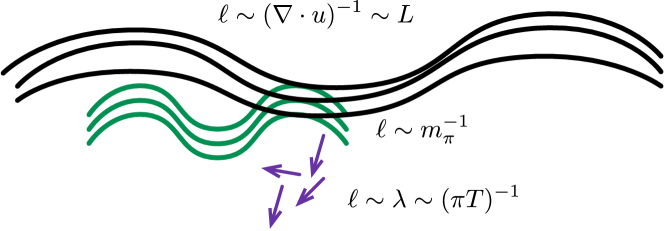
Figure 1: Long wavelength modes (black lines) with $\ell\sim(\nabla\cdot u)^{-1}\sim L$ are described with ordinary hydrodynamics. To model wavelengths of order $\ell\sim(m_{\pi})^{-1}$, the effective theory must treat the soft pion modes explicitly (green lines). These modes can be described with a non-abelian superfluid theory, due to the fact that the pions are Goldstone bosons. Finally, the microscopic degrees of freedom (purple arrows), which include typical pions with $p\sim\lambda^{-1}\sim\pi T$ and other hadronic states, determine the thermodynamic and dissipative parameters of the superfluid. The superfluid modes leave calculable imprints on the transport parameters of the ordinary fluid.

II.1 Ideal hydrodynamics

The hydrodynamic theory is based on the conserved charges and phases associated with broken $SU_{L}(2)\times SU_{R}(2)$. The invariance of the theory yields two conserved currents with independent left and right isospin rotations

$$J_{L}^{\mu}= (J_{L})_{a}^{\mu}t^{a}\,,$$ (1)

$$J_{R}^{\mu}= (J_{R})_{a}^{\mu}t^{a}\,,$$ (2)

where the generators $t^{a}$ are proportional to the Pauli matrices, with trace normalization ${\mathrm{tr}}[t^{a}t^{b}]=T_{F}\delta^{ab}$. The equilibrium state is characterized by the chiral condensate $\Sigma\equiv\left\langle\bar{q}_{R}q_{L}\right\rangle$, which transforms as $\Sigma\rightarrow g_{L}\Sigma g_{R}^{\dagger}$ under a chiral rotation. At each point in space and time, the local value chiral condensate $\Sigma\equiv\left\langle\bar{q}_{R}q_{L}\right\rangle(x)$ is rotated relative to a reference state $\Sigma^{(0)}=\sigma(T)\mathbb{I}$ by an axial rotation, where $g_{L}=g_{R}^{\dagger}=\xi$. The phase $\xi=\exp(i\varphi)$ is parametrized by the pion field $\varphi=\varphi_{a}(x)t^{a}$. Since under independent left and right rotations $\Sigma\rightarrow g_{L}\Sigma g_{R}^{\dagger}$, the condensate may be written $\Sigma=\sigma U$, where $U\equiv\xi^{2}$ is the phase, i.e. the unitary matrix that is traditionally used to parametrize the chiral Lagrangian. For the purposes of this paper, we will take $\sigma$ to be a constant. Fluctuations of $\sigma$ will be considered in future works.

As just discussed, the system at a point $x$ is rotated relative to a reference state by an $SU_{L}(2)\times SU_{R}(2)$ rotation parametrized by $(U_{L}(x),U_{R}(x))$. The left and right chemical potentials are related to time derivatives of these rotation matrices *[Thisdefinitionandchoiceofvariablesforthefluidactionwasinspiredby][]Glorioso:2018wxw,

$$\mu_{L} \equiv iu^{\mu}D_{\mu}^{{\mathscr{L}}}U_{L}U^{\dagger}_{L}=iu^{\mu}\partial_{\mu}U_{L}U_{L}^{\dagger}+u^{\mu}{\mathscr{L}}_{\mu},$$ (3)

$$\mu_{R} \equiv iu^{\mu}D_{\mu}^{{\mathscr{R}}}U_{R}U^{\dagger}_{R}=iu^{\mu}\partial_{\mu}U_{R}U_{R}^{\dagger}+u^{\mu}{\mathscr{R}}_{\mu},$$ (4)

where ${\mathscr{L}}_{\mu}$ and ${\mathscr{R}}_{\mu}$ are external left and right gauge fields, and the flow velocity $u^{\mu}$ is timelike normalized, $u^{\mu}u_{\mu}=-1$. These relations are called Josephson constraints in the superfluid theory. The chiral condensate $\Sigma$ is given by $\Sigma=U_{L}\,(\sigma\mathbb{I})\,U_{R}^{\dagger}$, and thus the unitary matrix $U$ is simply $U=U_{L}U_{R}^{\dagger}$. In constructing the chiral Lagrangian it is customary to introduce the left and right handed currents, $L_{\mu}\equiv iUD_{\mu}U^{\dagger}$ and $R_{\mu}\equiv iU^{\dagger}D_{\mu}U=-U^{\dagger}L_{\mu}U$, defined with the appropriate covariant derivatives

$$D_{\mu}U =\partial_{\mu}U-i{\mathscr{L}}_{\mu}U+iU{\mathscr{R}}_{\mu},$$ (5)

$$D_{\mu}U^{\dagger} =\partial_{\mu}U^{\dagger}+iU^{\dagger}{\mathscr{L}}_{\mu}-i{\mathscr{R}}_{\mu}U^{\dagger}.$$ (6)

Using these definitions, we find that the zeroth component of the left and right handed currents are related to the difference in chemical potentials

$$-u^{\mu}L_{\mu}= iu^{\mu}D_{\mu}UU^{\dagger}=\mu_{L}-U\mu_{R}U^{\dagger},$$ (7)

$$-u^{\mu}R_{\mu}= iu^{\mu}D_{\mu}U^{\dagger}U=\mu_{R}-U^{\dagger}\mu_{L}U.$$ (8)

These are analogous to the $U(1)$ superfluid Josephson relation, where $-u^{\mu}\partial_{\mu}\varphi=\mu$.

To quadratic order in $\mu_{L}$, $\mu_{R}$, and $L_{\mu}$, the $SU_{L}(2){\times}SU_{R}(2)$ invariants are $\mu_{L}^{2}+\mu_{R}^{2}$, $(\mu_{L}-U\mu_{R}U^{\dagger})^{2}$ and $L_{\mu}L^{\mu}$. Thus, a general action for ideal hydrodynamics close to the chiral limit is

$$S= \int\text{d}^{4}x\sqrt{-g}(p(T)+\mathcal{L}_{\text{superfluid}}),$$ (9)

where

$$\mathcal{L}_{\text{superfluid}}=\frac{1}{4T_{F}}{\mathrm{tr}}\big{[}{\chi_{0}}\,(\mu_{L}^{2}+\mu_{R}^{2})\big{]}+\\ \frac{1}{8T_{F}}{\mathrm{tr}}\big{[}{\chi_{1}}\,u^{\mu}u^{\nu}D_{\mu}UD_{\nu}U^{\dagger}-f^{2}D_{\mu}UD^{\mu}U^{\dagger}+f^{2}m^{2}(U\mathcal{M}^{\dagger}+\mathcal{M}U^{\dagger})\big{]},$$ (10)

Here we are tracing over isospin. $p(T)$ is the pressure as a function of temperature, defined through the vector $\beta^{\mu}$, i.e. $T{\equiv}(-\beta^{\mu}g_{\mu\nu}\beta^{\nu})^{-1/2}$ with $\beta^{\mu}=\frac{1}{T}u^{\mu}$. $\mathcal{M}$ is a fixed matrix which can be taken to be unity, and is responsible for the explicit breaking of chiral symmetry. Note that $m$ refers to the screening mass, which is directly related to the pole mass, $m_{p}^{2}\equiv v^{2}m^{2}$ Son and Stephanov (2002a). The coefficients $\chi_{0},\chi_{1},f$ and $m$ are functions of the temperature. For the purposes of this paper, ultimately we will work around a Minkowski background, $g_{\mu\nu}=\eta_{\mu\nu}$, and also turn the gauge fields off, ${\mathscr{L}}_{\mu}={\mathscr{R}}_{\mu}=0$. Similar Lagrangians considering $U(1)$ superfluids, and $U(1)$ vector and axial currents coupled to gauge fields, including a discussion about anomalies, can be found in Jensen et al. (2012, 2013).

The hydrodynamic equations are given by the conservation of the energy momentum tensor Son (2000),

$$\nabla_{\mu}T^{\mu\nu} =0,$$ (11)

with

$$T^{\mu\nu}=\frac{2}{\sqrt{-g}}\frac{\partial\mathcal{L}\sqrt{-g}}{\partial g_{\mu\nu}} =\varepsilon_{U}u^{\mu}u^{\nu}+\Delta^{\mu\nu}p_{U}+\frac{f^{2}}{8T_{F}}{\mathrm{tr}}\left(D^{\mu}UD^{\nu}U^{\dagger}+D^{\nu}UD^{\mu}U^{\dagger}\right),$$ (12)

where $\Delta^{\mu\nu}\equiv\eta^{\mu\nu}+u^{\mu}u^{\nu}$ is the projector onto the local rest frame, the redefined pressure is

$$p_{U} =p(T)+\mathcal{L}_{\text{superfluid}},$$ (13)

and the redefined energy density is given by a Legendre transform of $p_{U}$

$$\varepsilon_{U}=\varepsilon(T)+\left(-1+T\frac{\partial}{\partial T}+\mu_{L}^{a}\frac{\partial}{\partial\mu_{L}^{a}}+\mu_{R}^{a}\frac{\partial}{\partial\mu_{R}^{a}}\right)\mathcal{L}_{\text{superfluid}}.$$ (14)

When determining $\varepsilon_{U}$, the Lagrangian should be considered a function of the independent variables $T$, $\mu_{L}$, $\mu_{R}$, ${\mathrm{tr}}(\partial_{\mu}U\partial^{\mu}U^{\dagger})$, and ${\mathcal{M}}^{\dagger}U+{\mathcal{M}}U^{\dagger}$, and thus the $\chi_{1}$ term in the $\mathcal{L}$ should be written:

$$\chi_{1}{\mathrm{tr}}[u^{\mu}u^{\nu}D_{\mu}UD_{\mu}U^{\dagger}]=\chi_{1}{\mathrm{tr}}[(\mu_{L}-U\mu_{R}U^{\dagger})^{2}]\,.$$ (15)

The ideal equations of motion of the chiral degrees of freedom read

$$D_{\mu}^{{\mathscr{L}}}J_{L}^{\mu} =-\frac{f^{2}m^{2}}{8}i(U\mathcal{M}^{\dagger}-\mathcal{M}U^{\dagger}),$$ (16)

$$D_{\mu}^{{\mathscr{R}}}J_{R}^{\mu} =+\frac{f^{2}m^{2}}{8}i(\mathcal{M}^{\dagger}U-U^{\dagger}\mathcal{M}),$$ (17)

where the left and right currents are given by

$$J_{L}^{\mu} =\frac{\delta S}{\delta{\mathscr{L}}_{a\mu}}t^{a}=\frac{1}{2}{\chi_{0}}\mu_{{\scriptscriptstyle L}}u^{\mu}+\frac{1}{4}\chi_{1}(\mu_{\scriptscriptstyle L}-U\mu_{\scriptscriptstyle R}U^{\dagger})u^{\mu}+\frac{1}{4}f^{2}L^{\mu}\,,$$ (18)

$$J_{R}^{\mu} =\frac{\delta S}{\delta{\mathscr{R}}_{a\mu}}t^{a}=\frac{1}{2}{\chi_{0}}\mu_{{\scriptscriptstyle R}}u^{\mu}+\frac{1}{4}\chi_{1}(\mu_{{\scriptscriptstyle R}}-U^{\dagger}\mu_{\scriptscriptstyle L}U)u^{\mu}+\frac{1}{4}f^{2}R^{\mu}\,.$$ (19)

Note that the conserved isovector current for $\mathcal{M}$ unity (i.e. the real world) is given by $\tilde{J}_{V}^{\mu}=J^{\mu}_{L}+\mathcal{M}J^{\mu}_{R}\mathcal{M}^{\dagger}$. It is also useful to consider $J_{V}^{\mu}\equiv J^{\mu}_{L}+UJ^{\mu}_{R}U^{\dagger}$, the associated chemical potential $\mu_{V}\equiv(\mu_{L}+U\mu_{R}U^{\dagger})/2$, and corresponding axial definitions, $J_{A}^{\mu}\equiv J^{\mu}_{L}-UJ_{R}^{\mu}U^{\dagger}$ and $\mu_{A}\equiv(\mu_{\scriptscriptstyle L}-U\mu_{\scriptscriptstyle R}U^{\dagger})/2$, which can be interpreted as the projection of the current and chemical potentials onto the iso-vector and iso-axial-vector directions as seen from the reference state Jain (2017). These projected currents read

$$J_{\scriptscriptstyle V}^{\mu}= \chi_{0}\,\mu_{\scriptscriptstyle V}\,u^{\mu},$$ (20)

$$J_{{\scriptscriptstyle A}}^{\mu}= \chi_{A}^{\rm nrm}\,\mu_{\scriptscriptstyle A}\,u^{\mu}+{\textstyle\frac{1}{2}}f^{2}L^{\mu}\,.$$ (21)

where we have defined $\chi_{A}^{\rm nrm}\equiv\chi_{0}+\chi_{1}$. The form of the iso-vector current leads us to identify $\chi_{0}$ as the iso-vector susceptibility. The iso-axial-vector current consists of a normal component with susceptibility $\chi_{A}^{\rm nrm}$ and a superfluid component with susceptibility $f^{2}$. The total iso-vector-axial charge density, $-u_{\mu}J^{\mu}_{{\scriptscriptstyle A}}$, is the total axial susceptibility, $\chi_{{\scriptscriptstyle A}}\equiv(\chi_{A}^{\rm nrm}+f^{2})$, times the axial chemical potential, $\mu_{{\scriptscriptstyle A}}$.

II.2 Viscous corrections, entropy production, and noise

II.2.1 Viscous corrections and entropy production

The equations that we have considered so far are ideal. We will be interested in computing the viscous corrections to the energy momentum tensor due to the viscous effects of the chiral sector. This section extends Pujol and Davesne (2003); Jain (2017) by including the mass terms (which are very important in practice), and Son and Stephanov (2002a) by treating the theory non-linearly, which leads to an additional constraint.

To this end we write

$$T^{\mu\nu}= T^{\mu\nu}_{\text{ideal}}+\Pi^{\mu\nu}\,,$$ (22)

$$J^{\mu}_{L}= J^{\mu}_{L,\text{ideal}}+q_{L}^{\mu}\,,$$ (23)

$$J^{\mu}_{R}= J^{\mu}_{R,\text{ideal}}+q_{R}^{\mu}\,.$$ (24)

and allow for a viscous correction to the Josephson constraint

$$-\tfrac{1}{2}u^{\mu}L_{\mu}=\mu_{A}+\mu_{A}^{diss}\,.$$ (25)

The phenomenological currents should be proportional to the strains, and entropy production should be positive. We may choose the Landau frame such that

$$u_{\mu}q_{L}^{\mu}=u_{\mu}q_{R}^{\mu}=u_{\mu}\Pi^{\mu\nu}=0\,.$$ (26)

Finally, we will further decompose the stress tensor into shear and bulk strains

$$\Pi^{\mu\nu}=\pi^{\mu\nu}+\Pi\Delta^{\mu\nu}\,,$$ (27)

where $\pi^{\mu}_{\;\mu}=0$.

The entropy is defined by the energy density $e_{U}$, pressure $p_{U}$ and left and right density $n_{L/R}$:

$$s_{U}=\frac{e_{U}+p_{U}-\mu_{L}\cdot n_{L}-\mu_{R}\cdot n_{R}}{T},$$ (28)

where we introduced the shorthand, $\mu_{L}\cdot n_{L}={\rm tr}[\mu_{L}n_{L}]/T_{F}$. A straightforward analysis of entropy production using the equations of motion as seen in Appendix A yields

$$\partial_{\mu}\left(s_{U}u^{\mu}-\mu_{L}\cdot q_{L}^{\mu}-\mu_{R}\cdot q_{R}^{\mu}\right)=-\Pi^{\mu\nu}\,\partial_{\mu}\beta_{\nu}-q_{L}^{\mu}\cdot\partial_{\mu}\hat{\mu}_{L}-q_{R}^{\mu}\cdot\partial_{\mu}\hat{\mu}_{R}-\frac{\mu_{A}^{diss}}{T}\cdot\Theta_{s}\,,$$ (29)

where $\hat{\mu}\equiv\mu/T$. The superfluid expansion scalar in this expression is

$$\Theta_{s}=\left[\partial_{\mu}\left(\frac{f^{2}}{2}L^{\mu}\right)+\frac{f^{2}m^{2}}{4}\,i(U\mathcal{M}^{\dagger}-\mathcal{M}U^{\dagger})\right]\,,$$ (30)

and is given by the variation of the ideal action leaving the temperature, $\mu_{V}$, and $\mu_{A}$ fixed

$$\left(\delta S\right)_{\beta,\mu_{V},\mu_{A}}\equiv\int d^{4}x\,\left(-\tfrac{i}{2}\delta UU^{\dagger}\right)\cdot\Theta_{s}\,.$$ (31)

Requiring positivity of entropy production leads in the tensor sector to

$$\pi^{\mu\nu}= -\eta^{(0)}\,\sigma^{\mu\nu}\quad\mbox{with}\quad\eta\geq 0\,.$$ (32)

In the scalar sector there are two structures, leading to the constitutive relations

$$-\Pi =\zeta^{(0)}\,\nabla\cdot u+\zeta^{(1)}\,\mu_{A}\cdot\Theta_{s}\,,$$ (33)

$$-\mu_{A}^{\rm diss} =\zeta^{(1)}\,\mu_{A}\,\nabla\cdot u+\;\zeta^{(2)}\phantom{\cdot}\Theta_{s}\,.$$ (34)

For the quadratic form, $-(\Pi\,\nabla\cdot u+\mu^{diss}_{A}\cdot\Theta_{s})$, to be non-negative we must have

$$\zeta^{(0)}\geq 0,\qquad\zeta^{(2)}\geq 0,\qquad\zeta^{(0)}\zeta^{(2)}-(\zeta^{(1)})^{2}\mu_{A}^{2}\geq 0\,.$$ (35)

In the vector-sector we have

$$q_{V}^{\alpha}= -T\sigma_{I}^{(0)}\Delta^{\alpha\beta}(\partial_{\alpha}\hat{\mu}_{L}+U\,\partial_{\beta}\hat{\mu}_{R}\,U^{\dagger})/2\,,$$ (37a)

$$= -T\sigma_{I}^{(0)}\,\Delta^{\alpha\beta}\left((\partial_{\beta}\hat{\mu}_{V}-\tfrac{i}{2}[L_{\beta},\hat{\mu}_{V}])+\tfrac{i}{2}[L_{\beta},\hat{\mu}_{A}]\right)\quad\mbox{with}\quad\sigma_{I}^{(0)}\geq 0\,.$$ (37b)

In the pseudo-vector sector we have

$$q_{A}^{\alpha}= -T\sigma_{A}\Delta^{\alpha\beta}(\partial_{\alpha}\hat{\mu}_{L}-U\,\partial_{\beta}\hat{\mu}_{R}\,U^{\dagger})/2\,,$$ (38a)

$$= -T\sigma_{A}\Delta^{\alpha\beta}\left((\partial_{\beta}\hat{\mu}_{A}-\tfrac{i}{2}[L_{\beta},\hat{\mu}_{A}])+\tfrac{i}{2}[L_{\beta},\hat{\mu}_{V}]\right)\quad\mbox{with}\quad\sigma_{A}\geq 0\,.$$ (38b)

To summarize, the superfluid theory contains the three transport coefficients of the normal theory, $\eta^{(0)},\zeta^{(0)},\sigma_{I}^{(0)}$. In addition, it contains two parameters, $\zeta^{(2)}$ and $\sigma_{A}$, which describe the damping of the pions, and which will be parameterized below by axial charge diffusion coefficient $D_{A}$ and the damping rate $D_{m}$. Finally, the theory contains one additional coefficient, $\zeta^{(1)}$ that intrinsically couples the normal and pion sectors. This term involves two small parameters, the axial chemical potential $\mu_{A}$ and the viscous correction arising from $\nabla\cdot u$, and can probably be ignored in practice.

It is notable that the two independent scalars comprising the superfluid expansion scalar, $\partial_{\mu}(f^{2}L^{\mu})$ and $U\mathcal{M}^{\dagger}-\mathcal{M}U^{\dagger}$, must have the same dissipative coefficient, $\zeta^{(2)}$. This constraint, arising from entropy considerations, was not recognized in the linearized analysis of dissipation by Son and Stephanov Son and Stephanov (2002a), which leads to an additional transport coefficient in their theory.

This consequence of entropy conservation simplifies the interpretation of the theory. For simplicity of presentation, we will set $\zeta^{(1)}$, $\sigma_{A}$, and $\sigma_{I}^{(0)}$ to zero, and call $\Gamma_{\rm chem}\equiv 1/\zeta^{(2)}$. (These constraints are all easily relaxed.) The chemical potential of the normal components is $\mu_{A}$, while the chemical potential of the pion component is $\mu_{A}^{\varphi}\equiv-\tfrac{1}{2}u^{\mu}L_{\mu}$, and the two potentials are trying to be made equal by the microscopic dynamics. From this perspective it is not surprising that the equations of motion can be easily rewritten in an intuitive form

$$\partial_{\mu}(n_{L}u^{\mu})\,-\,U\,\partial_{\mu}(n_{R}u^{\mu})\,U^{\dagger}= -\Gamma_{\rm chem}\left(\mu_{A}-\mu_{A}^{\varphi}\right),$$ (39)

$$\partial_{\mu}\left(\tfrac{f^{2}}{2}L^{\mu}\right)+\frac{f^{2}m^{2}}{4}i(U\mathcal{M}^{\dagger}-\mathcal{M}U^{\dagger})= -\Gamma_{\rm chem}\left(\mu_{A}^{\varphi}-\mu_{A}\right),$$ (40)

which clearly shows the chemical coupling between the pion equation of motion (40) and the normal axial components (i.e. hard pions and other hadronic states).

II.2.2 Noise

The analysis of entropy production also determines the thermodynamic noise in the system. Neglecting $\zeta^{(1)}$ for simplicity, the mean entropy production rate can be written

$$\partial_{\mu}\left(s_{U}u^{\mu}-\mu_{V}\cdot q_{V}^{\mu}-\mu_{A}\cdot q_{A}^{\mu}\right)=\frac{\pi^{\mu\nu}\pi_{\mu\nu}}{2T\eta^{(0)}}+\frac{\Pi^{2}}{T\zeta^{(0)}}+\frac{q_{V}^{\mu}(q_{V})_{\mu}}{T\sigma_{V}^{(0)}}+\frac{q_{A}^{\mu}(q_{A})_{\mu}}{T\sigma_{A}}+\frac{(\mu_{A}^{diss})^{2}}{T\zeta^{(2)}}\ .$$ (41)

In stochastic hydro, noise should be added to each dissipative strain, i.e.

$$q_{A}^{\mu} \rightarrow q_{A}^{\mu}+\xi_{A}^{\mu}\,,$$ (42a)

$$\mu_{A}^{diss} \rightarrow\mu_{A}^{diss}+\xi_{\mu_{A}}^{diss}\,,$$ (42b)

in addition to the familiar noises of ordinary hydrodynamics, $\xi^{\mu\nu}_{\pi}$, $\xi_{\Pi}$, and $\xi_{V}^{\mu}$. The general theory of these fluctuations determines the variances of the noises from the equilibrium susceptibility matrix and the dissipative quadratic form for entropy production Landau and Lifshitz (2013); Landau et al. (1980); Fox and Uhlenbeck (1970a, b). In the current case, these variances can be read off from the denominators of (41), i.e.

$$\left\langle\xi^{\mu}_{A}(x)\xi_{A}^{\nu}(y)\right\rangle =2T\sigma_{A}\Delta^{\mu\nu}\delta(x-y)\,,$$ (43a)

$$\left\langle\xi_{\mu_{A}}^{diss}(x)\xi_{\mu_{A}}^{diss}(y)\right\rangle =2T\zeta^{(2)}\delta(x-y)\,.$$ (43b)

in addition to the usual variances for $\xi^{\mu\nu}_{\pi}$, $\xi_{\Pi}$, and $\xi_{V}^{\mu}$. In writing these formulae in this simple form it was important that we expanded $\mu^{diss}_{A}$ in terms of the canonical conjugate of $U$, as given by $\Theta_{s}$ in (31). Otherwise, the form of the variances would also involve the equilibrium matrix of susceptibilities.

Finally, we note that in the presence of noise, the rearrangements of the equations of motion that lead to (39) and (40) now give rise to a stochastic equation of chemical balance

$$\partial_{\mu}(n_{L}u^{\mu})\,-\,U\,\partial_{\mu}(n_{R}u^{\mu})\,U^{\dagger}= -\Gamma_{\rm chem}\left(\mu_{A}-\mu_{A}^{\varphi}\right)-\xi_{\rm chem},$$ (44)

$$\partial_{\mu}\left(\tfrac{f^{2}}{2}L^{\mu}\right)+\frac{f^{2}m^{2}}{4}i(U\mathcal{M}^{\dagger}-\mathcal{M}U^{\dagger})= -\Gamma_{\rm chem}\left(\mu_{A}^{\varphi}-\mu_{A}\right)+\xi_{\rm chem},$$ (45)

where the chemical noise $\xi_{\rm chem}$ (which enters as $\Gamma_{\rm chem}\,\xi_{\mu_{A}}^{diss}$) satisfies the expected chemical fluctuation-dissipation relation

$$\left\langle\xi_{\rm chem}(x)\xi_{\rm chem}(y)\right\rangle =(\Gamma_{\rm chem})^{2}\left\langle\xi_{\mu_{A}}^{diss}(x)\,\xi_{\mu_{A}}^{diss}(y)\right\rangle\,,$$ (46a)

$$=2T\,\Gamma_{\rm chem}\,\delta(x-y)\,,$$ (46b)

confirming the consistency of the interpretation.

II.3 Linearized equations of motion

Following Son and Stephanov Son and Stephanov (2002a), we now parametrize the phase as $U=e^{2i\varphi}$ and linearize the equation of motion for $J_{A}^{\mu}$ together with the Josephson’s constraint around global equilibrium:

$$\partial_{t}(\chi_{A}^{\rm nrm}\mu_{A})+\nabla\cdot(-\sigma_{A}\nabla\mu_{A}+\vec{\xi}_{A})= -\Gamma_{\rm chem}(\mu_{A}-\mu_{A}^{\varphi})-\xi_{\rm chem}\,,$$ (47)

$$-\partial_{t}(f^{2}\partial_{t}\varphi)+\nabla\cdot(f^{2}\nabla\varphi)-f^{2}m^{2}\varphi= -\Gamma_{\rm chem}(\mu_{A}^{\varphi}-\mu_{A})+\xi_{\rm chem}\,,$$ (48)

with $\mu_{A}^{\varphi}=-\partial_{t}\varphi$. After using lower order equations of motion, the stochastic equation for the pion field reads (see Appendix B)

$$\chi_{A}\partial_{t}^{2}\varphi-f^{2}\partial_{i}^{2}\varphi+f^{2}m^{2}\varphi-\lambda_{A}\nabla^{2}\partial_{t}\varphi+\lambda_{m}m^{2}\,\partial_{t}\varphi=\xi,$$ (49)

where $\lambda_{A}$ and $\lambda_{m}$ are related to the coefficients described above (with $\Gamma_{\rm chem}\equiv 1/\zeta^{(2)}$):

$$\lambda_{A} \equiv\sigma_{A}+(\chi_{A}^{\rm nrm}v)^{2}\,\zeta^{(2)}\,,$$ (50)

$$\lambda_{m} \equiv(\chi_{A}^{\rm nrm}v)^{2}\,\zeta^{(2)}\,,$$ (51)

and the noise $\xi$ satisfies the fluctuation-dissipation relation:

$$\left\langle\xi(x)\xi(y)\right\rangle=2T(-\lambda_{A}\nabla^{2}+\lambda_{m}m^{2})\,\delta(x-y)\,.$$ (52)

The equation of motion can be used to evaluate the corresponding propagators. We will need the symmetrized correlation function

$$G_{ab,\rm sym}^{\varphi\varphi}(\omega,{\bm{q}})\equiv\int d^{4}x\,e^{i\omega t-i{\bm{q}}\cdot{\bm{x}}}\left\langle\varphi_{a}(t,{\bm{x}})\varphi_{b}(0)\right\rangle\equiv\delta_{ab}G_{\rm sym}^{\varphi\varphi}.$$ (53)

The retarded response function associated with the left hand side of (49) is

$$G_{R}^{\varphi\varphi}(\omega,{\bm{q}}) =\frac{1}{\chi_{A}}\frac{1}{-\omega^{2}+\omega_{q}^{2}-i\omega\Gamma_{q}},$$ (54)

$$\omega_{q}^{2} \equiv v^{2}(q^{2}+m^{2}),$$ (55)

where the pion velocity is given by $v^{2}=\frac{f^{2}}{\chi_{A}}$ and the attenuation is defined as

$$\Gamma_{q} \equiv D_{A}q^{2}+D_{m}m^{2},\qquad\text{where}\qquad D_{A}\equiv\frac{\lambda_{A}}{\chi_{A}},\qquad\text{and}\qquad D_{m}\equiv\frac{\lambda_{m}}{\chi_{A}}.$$ (56)

$D_{A}$ and $D_{m}$ are the axial charge diffusion and damping coefficients, respectively. Using the fluctuation-dissipation relation, or equivalently by solving (49) with the noise, we can obtain the symmetrized correlation function,

$$G_{\rm sym}^{\varphi\varphi} =\frac{1}{\chi_{A}}\frac{2T\Gamma_{q}}{(-\omega^{2}+\omega_{q}^{2})^{2}+(\Gamma_{q}\omega)^{2}}\,.$$ (57)

The propagator is sharply peaked near the poles leading to an approximate expression

$$G_{\rm sym}^{\varphi\varphi}\simeq\frac{T}{2\chi_{A}\omega_{q}^{2}}\left[\rho(\omega,\omega_{q})+\rho(\omega,-\omega_{q})\right],$$ (58)

where

$$\rho=\frac{\Gamma_{q}}{(-\omega+\omega_{q})^{2}+(\Gamma_{q}/2)^{2}}.$$ (59)

This approximation is justified when the imaginary part of the dispersion relation, $\Gamma_{q}$, is negligible with respect to its real part $\omega_{q}$, i.e. $\Gamma_{q}/\omega_{q}\ll 1$.

III Dependence of the transport coefficients of QCD on the pion mass

Here we will first use the Kubo formula to deduce the dependence of the shear viscosity, $\eta$, bulk viscosity, $\zeta$, and iso-vector conductivity, $\sigma_{I}$, on the pion mass. The technical step is to integrate out the pion loop shown below to determine the corresponding fluctuations in the stress tensor or current.

Figure 2: An example of a hydrodynamic pion loop in Kubo furmulae.

An equivalent approach to superfluid hydrodynamic loops is to develop a hydro-kinetic equation for the soft pions Akamatsu et al. (2017); An et al. (2019). In this case the phase space distribution of soft pions evolves according to a Boltzmann equation with the normal fluid driving the distribution function out of equilibrium. The collision kernel of Boltzmann equation is determined by the axial charge diffusion and damping coefficients of the superfluid, $D_{A}$ and $D_{m}$, respectively. A distinct advantage of the hydro-kinetic approach is that it can be simulated in expanding environments, capturing the physics associated with the chiral fluctuations. We will describe this approach in Sect. III.2 after analyzing the hydrodynamic loop.

III.1 Kubo Formulae

The three transport coefficients of interest here are expressed as Forster (1995)

$$2T\eta= \int d^{4}x\left\langle{\textstyle\frac{1}{2}}\{T^{xy}(t,{\bm{x}}),T^{xy}(0,{\bm{0}})\}\right\rangle,$$ (60)

$$2T\sigma_{I}= \int d^{4}x\frac{1}{d_{A}}\left\langle{\textstyle\frac{1}{2}}\{J_{V,a}^{x}(t,{\bm{x}}),J_{V,a}^{x}(0,{\bm{0}})\}\right\rangle,$$ (61)

$$2T\zeta= \int d^{4}x\left\langle{\textstyle\frac{1}{2}}\left\{{\mathcal{O}}_{\rm bulk}(t,{\bm{x}}),{\mathcal{O}}_{\rm bulk}(0,{\bm{0}})\right\}\right\rangle.$$ (62)

Here $d_{A}=3$ is the dimension of the adjoint and we are summing over the isospin index. In determining the bulk viscosity is very convenient to use the operator

$$\mathcal{O}_{\rm bulk}\equiv c_{s}^{2}T^{0}_{\phantom{0}0}+\frac{1}{3}T^{i}_{\phantom{i}i},$$ (63)

where $c_{s}^{2}$ is a fixed parameter for the system at temperature $T$. This operator has several related advantages over $T^{\mu}_{\;\mu}$ Jeon and Yaffe (1996). Specifically, it is invariant in equilibrium under small shifts in the temperature, and therefore it is not necessary to impose the Landau matching condition when perturbing the system. It also behaves smoothly as the spatial momentum ${\bm{k}}\rightarrow 0$, while $T^{\mu}_{\;\mu}$ does not Romatschke and Son (2009); Hong and Teaney (2010).

To evaluate the pion contributions to these correlations we will need the symmetrized correlation function discussed in the previous section and more explicit expressions for the operators of interest. Here we have

$$T^{xy}= f^{2}\partial^{x}\varphi_{a}\partial^{y}\varphi_{a},$$ (64)

$$J_{V,a}^{x}= -f^{2}f_{abc}\partial^{x}\varphi_{b}\varphi_{c},$$ (65)

$${\mathcal{O}}_{\rm bulk}= \left[p_{\varphi}+\frac{1}{3}f^{2}(\nabla\varphi_{a})^{2}-c_{s}^{2}\left({\chi_{A}}(\partial_{t}\varphi_{a})^{2}-\frac{\partial(\beta p_{\varphi})}{\partial\beta}\right)\right],$$ (66)

$$p_{\varphi}= \frac{1}{2}\chi_{A}\left[(\partial_{t}\varphi_{a})^{2}-v^{2}(\nabla\varphi_{a})^{2}-v^{2}m^{2}\varphi_{a}^{2}\right].$$ (67)

Evaluating the Feynman graphs for the shear stress, current, and bulk operator gives

$$2T\eta =2T\eta^{(0)}(\Lambda)+2d_{A}f^{4}\int^{\Lambda}\frac{dq^{0}d^{3}q}{(2\pi)^{4}}\,(q^{x}q^{y})^{2}\,(G^{\varphi\varphi}_{\rm sym}(q^{0},q))^{2},$$ (68)

$$2T\sigma_{I} =2T\sigma_{I}^{(0)}(\Lambda)+2T_{A}f^{4}\int^{\Lambda}\frac{dq^{0}d^{3}q}{(2\pi)^{4}}\,(q^{x})^{2}\,(G^{\varphi\varphi}_{\rm sym}(q^{0},q))^{2},$$ (69)

$$2T\zeta =2T\zeta^{(0)}(\Lambda)+2d_{A}\int^{\Lambda}\frac{dq^{0}d^{3}q}{(2\pi)^{4}}\,(\mathcal{N}_{\rm bulk}(q_{0},q))^{2}\,(G^{\varphi\varphi}_{\rm sym}(q^{0},q))^{2},$$ (70)

where $T_{A}=2$ is the trace of the adjoint. The numerator algebra associated with the operator ${\mathcal{O}}_{\rm bulk}$ evaluates to

$${\mathcal{N}}_{\rm bulk}={\textstyle\frac{1}{2}}\left({\chi_{A}}+c_{s}^{2}\frac{\partial(\beta{\chi_{A}})}{\partial\beta}\right)\,(q_{0}^{2}-\omega_{q}^{2})+\frac{{\chi_{A}}}{3}v^{2}q^{2}-c_{s}^{2}{\chi_{A}}\left(q_{0}^{2}+\frac{\beta}{2}\frac{\partial\omega_{q}^{2}}{\partial\beta}\right).$$ (71)

For each integral we will perform the $q^{0}$ integration first. The propagators are sharply peaked near $q^{0}=\pm\omega_{q}$, and cross terms in $(G^{\varphi\varphi}_{\rm sym})^{2}$ can be neglected in the integration. Performing the $q_{0}$ integral we find

$$\eta =\eta^{(0)}(\Lambda)+d_{A}\int^{\Lambda}\frac{d^{3}q}{(2\pi)^{3}}\left(\frac{\partial\omega_{q}}{\partial q_{x}}q_{y}\right)^{2}\left(\frac{T}{\omega_{q}^{2}}\right)\frac{1}{\Gamma_{q}},$$ (72a)

$$\sigma_{I} =\sigma_{I}^{(0)}(\Lambda)+T_{A}\int\frac{d^{3}q}{(2\pi)^{3}}\left(\frac{\partial\omega_{q}}{\partial q_{x}}\right)^{2}\left(\frac{T}{\omega_{q}^{2}}\right)\frac{1}{\Gamma_{q}},$$ (72b)

$$\zeta =\zeta^{(0)}(\Lambda)+d_{A}\int^{\Lambda}\frac{d^{3}q}{(2\pi)^{3}}\left[\frac{{\bm{q}}}{3}\cdot\frac{\partial\omega_{q}}{\partial{\bm{q}}}-c^{2}_{s}\frac{\partial(\beta\omega_{q})}{\partial\beta}\right]^{2}\left(\frac{T}{\omega_{q}^{2}}\right)\frac{1}{\Gamma_{q}}.$$ (72c)

As is briefly described in the next subsection these expressions are familiar from kinetic theory.

These integrals depend on the two transport coefficients, $D_{A}$ and $D_{m}$, the thermodynamic properties of the soft pions, $m_{p}^{2}=v^{2}m^{2}$ and $v^{2}=f^{2}/\chi_{A}$, as well as the speed of sound squared, $c_{s}^{2}$, which can be determined from the Euclidean measurements. These quantities enter in the final results as

$$\tilde{v}^{2} =v^{2}-\frac{T}{2}\frac{\partial v^{2}}{\partial T},$$ (73)

$$\tilde{m}_{p}^{2} =m_{p}^{2}-\frac{T}{2}\frac{\partial m^{2}_{p}}{\partial T},$$ (74)

and via a dimensionless ratio

$$r=\sqrt{\frac{D_{m}}{D_{A}}}.$$ (75)

It is worthwhile to point out that in chiral perturbation theory $r=\sqrt{4/3}$ Teaney et al. .

Evaluating the integrals, we find the final expressions to the corrections of the transport coefficients:

$$\zeta= \zeta^{(0)}_{\rm phys}+\frac{d_{A}Tm}{8\pi D_{A}}\left[\left(\frac{c_{s}^{2}}{1+r}\,\frac{\tilde{m}^{2}_{p}}{m^{2}_{p}}-\frac{1+2r}{1+r}\left(\tfrac{1}{3}-c_{s}^{2}\frac{\tilde{v}^{2}}{v^{2}}\right)\right)^{2}-(4+2r)\left(\tfrac{1}{3}-c_{s}^{2}\frac{\tilde{v}^{2}}{v^{2}}\right)^{2}\right],$$ (76a)

$$\eta= \eta^{(0)}_{\rm phys}-\frac{d_{A}Tm}{120\pi D_{A}}\left[\frac{2r^{3}+4r^{2}+6r+3}{(1+r)^{2}}\right],$$ (76b)

$$\sigma_{I}= (\sigma_{I})^{(0)}_{\rm phys}+\frac{T_{A}T}{24\pi mD_{A}}\left[\frac{1+2r}{(1+r)^{2}}\right].$$ (76c)

Here the shear viscosity and the bulk viscosity are renormalized quantities

$$\zeta^{(0)}_{\rm phys}= \zeta^{(0)}(\Lambda)+\frac{d_{A}T\Lambda}{2\pi^{2}D_{A}}\left(\tfrac{1}{3}-c_{s}^{2}\frac{\tilde{v}^{2}}{v^{2}}\right)^{2},$$ (77a)

$$\eta^{(0)}_{\rm phys}= \eta^{(0)}(\Lambda)+\frac{d_{A}T\Lambda}{30\pi^{2}D_{A}}.$$ (77b)

In each case, the “zero” transport coefficients (e.g. $\zeta^{(0)}$) are the parameters in the chiral limit, $m_{q}=0$. The conductivity $\sigma_{I}$ is not renormalized, and its soft pion contribution is proportional to the inverse screening mass, $m^{-1}$. This contribution diverges in the chiral limit and is parametrically larger than $(\sigma_{I})_{\rm phys}^{(0)}$. This reflects the fact that in this limit the soft pion is a free particle which transports isospin.

As emphasized in Son and Stephanov (2002a) many of the parameters in (76) can be evaluated on the lattice Brandt et al. (2014). Indeed all of the parameters of the ideal superfluid hydro, such as $v^{2},c_{s}^{2},m_{p}^{2}$ and $m^{2}$, are amenable to a Euclidean computation, while the viscous parameters $D_{A}$ and $r$ must be extracted from data or estimated from theoretical considerations. We will analyze the behavior of eq. (76) near the $O(4)$ critical point in Sect. IV.

III.2 Kinetic approach

The physical content of hydrodynamic loop calculations, such as described in the previous section, are (always) equivalent to deriving a Boltzmann equation for the hard sound modes in the plasma and using this Boltzmann equation to analyze the response Akamatsu et al. (2017); An et al. (2019). Indeed, our results for the transport coefficients (76) are much more transparently obtained from a hydro-kinetic Boltzmann equation for the soft pion phase-space distribution function $f_{\pi}(x,q_{i})$, which takes the form of a relaxation time like approximation. We are motivated by a similar Boltzmann equation for sound modes in normal hydrodynamics An et al. (2019).

First we generalize the linear analysis of the previous section to a flowing fluid background in Appendix B, using the scale separation depicted in Fig. 1. The ideal terms in the equation of motion are of order $\partial^{2}\varphi\sim m^{2}\varphi$, while flow corrections to these terms are of order $(\partial\varphi)(\partial u)\sim m\varphi/L$. Denoting the mean free path $\lambda$, the dissipative terms in the equation of motion are of order $\lambda\partial^{3}\varphi\sim\lambda m^{3}\varphi$, while flow corrections to these terms are of order $(\lambda/L)m^{2}$ and are ignored. We are thus working in a kinetic regime where

$$(\lambda/L)m^{2}\ll(m/L)\sim\lambda m^{3}\ll m^{2}\,.$$ (78)

With these approximations the stochastic wave equation takes the form

$$-\partial_{\mu}({\chi_{A}}\,G^{\mu\nu}\partial_{\nu}\varphi)+f^{2}m^{2}\varphi-\lambda_{A}\nabla_{\perp}^{2}\partial_{\tau}\varphi+\lambda_{m}m^{2}\partial_{\tau}\varphi=\xi\,.$$ (79)

Here $\nabla_{\perp}^{\mu}\equiv\Delta^{\mu\nu}\partial_{\nu}$ and $\partial_{\tau}=u^{\mu}\partial_{\mu}$ are the local spatial and temporal derivatives, and the pion field moves in an effective metric created by the flowing fluid

$$G^{\mu\nu}(x)\equiv-u^{\mu}(x)u^{\nu}(x)+v^{2}(x)\Delta^{\mu\nu}(x)\,,$$ (80)

where $v^{2}(x)\equiv f^{2}/\chi_{A}$ is the local pion velocity.

Appendix C shows that under the evolution of the stochastic wave equation, the pion phase-space distribution $f_{\pi}(x,q_{i})$ evolves according to a Boltzmann equation which takes the form

$$\frac{\partial\mathcal{H}}{\partial q_{\mu}}\,\frac{\partial f_{\pi}}{\partial x^{\mu}}-\frac{\partial\mathcal{H}}{\partial x^{i}}\,\frac{\partial f_{\pi}}{\partial q_{i}}=-\Gamma_{q}\left[\omega_{q}\,f_{\pi}-T\right]\,,$$ (81)

where the effective Hamiltonian,

$$\mathcal{H}(x,q)=\frac{1}{2}G^{\mu\nu}(x)q_{\mu}q_{\nu}+\frac{1}{2}v^{2}(x)m^{2}(x)\,,$$ (82)

is a function of the four vectors $x$ and $q$. Given the covariant momenta $q_{i}$, the covariant energy component $q_{0}$ is found by solving the on-shell constraint, $\mathcal{H}(x,q)=0$, taking the negative root $q_{0}=-h_{+}(x,q_{i})$, see (158). The components $G^{\mu\nu}q_{\nu}=\partial\mathcal{H}/\partial q_{\mu}$ should be distinguished from $q^{\mu}\equiv\eta^{\mu\nu}q_{\nu}$. The damping rate $\Gamma_{q}$ and dispersion curve $\omega_{q}=-u^{\mu}q_{\mu}$ are to be evaluated in the rest frame of the fluid, see (152). The equilibrium distribution is simply the classical part of the Bose-Einstein distribution function, $T/\omega_{q}$. We note that the Boltzmann equation can also be written

$$\frac{\partial\mathcal{H}}{\partial q_{0}}\,\left[\frac{\partial f_{\pi}}{\partial t}+\frac{\partial h_{+}}{\partial q_{i}}\frac{\partial f_{\pi}}{\partial x^{i}}-\frac{\partial h_{+}}{\partial x^{i}}\frac{\partial f_{\pi}}{\partial q_{i}}\right]=-\Gamma_{q}\left[\omega_{q}\,f_{\pi}-T\right]\,.$$ (83)

Once the phase space distribution is found, the pion contribution to the stress tensor is given by the superfluid stress in (12). Recalling that the phase space distribution $f_{\pi}(x,q_{i})$ is the Wigner transform of the noise averaged two point function $\left\langle\varphi(x)\varphi(y)\right\rangle$, Appendix C.2 shows that pion contribution to average stress tensor evaluates to

$$T^{\mu\nu}_{\pi}=d_{A}\int\frac{d^{3}q_{i}}{(2\pi)^{3}(\partial\mathcal{H}/\partial q_{0})}\left[\omega_{q}\frac{\partial(\beta\omega_{q})}{\partial\beta}u^{\mu}u^{\nu}+v^{2}\Delta^{\mu\alpha}\Delta^{\nu\beta}q_{\alpha}q_{\beta}\right]f_{\pi}(x,q_{i})\,.$$ (84)

Given this Boltzmann equation for the soft pion distribution and the stress tensor, familiar steps from the relaxation time approximation lead to the shear and bulk viscosities presented in (72) with relaxation time $1/\Gamma_{q}$ and dispersion curve $\omega_{q}$. We have not derived the isospin conductivity using the kinetic approach in this paper.

IV Discussion and behavior near the chiral critical point

In this section we will estimate our results for the transport coefficients, eq. (76), near the $O(4)$ critical point.

IV.1 The chiral phase transition: a brief review

First we review the expected scaling behavior of various quantities following Son and Stephanov (2002b); Rajagopal and Wilczek (1993b). The order parameter, $\sigma(x)\equiv\bar{\psi}\psi(x)$, and the inverse correlation length, $m_{\sigma}$, have the following scaling behavior near the critical point

$$\langle\bar{\psi}\psi\rangle\sim t^{\beta},\quad m_{\sigma}\sim t^{\nu},$$ (85)

where the reduced temperature is $t=|T-T_{c}|/T_{c}$, and $\beta$ and $\nu$ are the usual critical exponents. In the vicinity of the critical point, the static correlation function of the order parameter behaves like

$$\int d^{3}x\;e^{-i{\bm{x}}\cdot{\bm{q}}}\,\langle\sigma({\bm{x}})\sigma(0)\rangle\sim\frac{T}{|{\bm{q}}|^{2-\eta}},$$ (86)

for momentum, $|{\bm{q}}|$, much larger than $m_{\sigma}$, but smaller than the temperature $T$, $m_{\sigma}\ll|{\bm{q}}|\ll T$. The critical exponent $\eta$ is small in practice, and can be related to $\beta$ and $\nu$ using the hyperscaling relation

$$2\beta=\nu\left(d-2+\eta\right),$$ (87)

where $d=3$ is the spatial dimension. Finally, the order parameter relaxation rate scales with correlation length as Rajagopal and Wilczek (1993b)

$$\Gamma_{\sigma}\sim(m_{\sigma})^{z},$$ (88)

where $z=d/2$ is the dynamical critical exponent. As we will describe in the next paragraphs, $\Gamma_{\sigma}$ is of order $D_{A}m_{\sigma}^{2}$, and therefore we will define $\Gamma_{\sigma}\equiv D_{A}m_{\sigma}^{2}$ in our estimates below. A summary of the relevant scalings can be found in Table 1.

physical quantity	symbol	scaling	estimate
order parameter	$\left\langle\sigma\right\rangle=\langle\bar{\psi}\psi\rangle$	$t^{\beta}$	$\beta\simeq 0.380$
inverse correlation length	$m_{\sigma}$	$t^{\nu}$	$\nu\simeq 0.738$
static correlation function	$\int d^{3}x\;e^{-i{\bm{x}}\cdot{\bm{q}}}\,\langle\sigma({\bm{x}})\sigma(0)\rangle$	$T|{\bm{q}}|^{\eta-2}$	$\eta\simeq 0.03$
$\sigma$ relaxation rate	$\Gamma_{\sigma}\equiv D_{A}m_{\sigma}^{2}$	$m_{\sigma}^{z}$	$z=\frac{d}{2}$
axial susceptibility	$\chi_{A}$	$\chi_{0}$	const
$(\mbox{pion velocity})^{2}$	$v^{2}{=}f^{2}/\chi_{A}$	$t^{\nu(d-2)}$	$t^{0.738}$
$(\mbox{screening mass})^{2}$	$m^{2}$	$m_{q}t^{\beta-(d-2)\nu}$	$m_{q}\,t^{-0.358}$
$(\mbox{pole mass})^{2}$	$m^{2}_{p}{=}v^{2}m^{2}$	$m_{q}t^{\beta}$	$m_{q}\,t^{0.380}$

Table 1: Here we list the critical scaling of relevant parameters near the chiral critical point, as discussed in Son and Stephanov (2002b).

In the chirally broken phase close to $T_{c}$, but not so close that fluctuations in $\sigma$ are important, the Lagrangian in eq. (10) applies. The static pion propagator $\pi_{a}=\left\langle\bar{\psi}\psi\right\rangle\varphi_{a}$ at momentum scale $m\ll|{\bm{q}}|\ll m_{\sigma}$ can be read off from the Euclidean version of the Lagrangian

$$\int d^{3}x\;e^{-i{\bm{x}}\cdot{\bm{q}}}\,\langle\pi_{a}({\bm{x}})\pi_{b}(0)\rangle\approx\delta_{ab}\frac{T\langle\bar{\psi}\psi\rangle^{2}}{f^{2}}\frac{1}{|{\bm{q}}|^{2}}.$$ (89)

In the vicinity of the phase transition, the $\pi$ and $\sigma$ propagators become degenerate. Thus, the scaling of the two propagators (eq. (86) and eq. (89)) must be the same at their boundaries of applicability $|{\bm{q}}|\sim m_{\sigma}$, leading to a relation between the pion decay constant $f^{2}$ , $m_{\sigma}^{2}$, and $\langle\bar{\psi}\psi\rangle$,

$$f^{2}\sim m_{\sigma}^{-\eta}\langle\bar{\psi}\psi\rangle^{2}\sim t^{\nu(d-2)}.$$ (90)

Then the pion velocity near $T_{c}$ scales like

$$v^{2}=\frac{f^{2}}{\chi_{A}}\sim t^{\nu(d-2)},$$ (91)

where $\chi_{A}\simeq\chi_{0}$ is approximately constant near $T_{c}$. The screening mass, $m$, can be related to the pion decay constant $f^{2}$, the condensate $\left\langle\bar{\psi}\psi\right\rangle$, and the quark mass $m_{q}$ via

$$m^{2}=-m_{q}\frac{\langle\bar{\psi}\psi\rangle}{f^{2}}\sim m_{q}t^{\beta-(d-2)\nu}.$$ (92)

Similarly, the pole mass scales like

$$m_{p}^{2}=v^{2}m^{2}=-m_{q}\frac{\langle\bar{\psi}\psi\rangle}{\chi_{\scriptscriptstyle A}}\sim m_{q}t^{\beta}\,.$$ (93)

Close to $T_{c}$, but again not so close that $\sigma$ fluctuates, the hydrodynamic analysis applies and the pion dispersion curve for $q\gg m$ reads

$$\omega(q)=v|{\bm{q}}|-\tfrac{i}{2}D_{A}q^{2}\,.$$ (94)

As we approach the phase transition, the real and imaginary parts of the dispersion curve become the same order of magnitude. Also, the pion and $\sigma$ damping rates should scale similarly near $T_{c}$ at the boundaries of applicability $|{\bm{q}}|\sim m_{\sigma}$. This reasoning yields the following estimates

$$vm_{\sigma}\sim D_{A}m_{\sigma}^{2}\sim(m_{\sigma})^{z}\,.$$ (95)

For definiteness we will define the relaxation rate $\Gamma_{\sigma}$ using the axial charge diffusion coefficient $\Gamma_{\sigma}\equiv D_{A}m_{\sigma}^{2}$. The temperature scaling of $D_{A}$ is

$$D_{A}\sim t^{\nu(\frac{d}{2}-2)}=t^{-\nu/2}.$$ (96)

IV.2 The transport coefficients near $T_{c}$

Armed with these scaling relations, we can determine the temperature and quark mass dependence of the transport coefficients near $T_{c}$. We are assuming that we are not so close to $T_{c}$ that the $\sigma$ field fluctuates strongly. The $\sigma$ fluctuations cannot be neglected when the screening mass in (92) becomes of order $m_{\sigma}$, which yields

$$\frac{m}{m_{\sigma}}\sim\sqrt{m_{q}}\,t^{(\beta-3\nu)/2}\,,$$ (97)

and therefore the analysis breaks down when $t\sim(\sqrt{m_{q}})^{1.091}$. Since the pion mass $m_{\pi}\propto\sqrt{m_{q}}$ is fairly massive compared to, e.g. $2\pi T_{c}$, it is likely that $\sigma$ fluctuations can never be completely ignored over the temperature range relevant to heavy ion collisions.

Nevertheless, we wish to evaluate the temperature and quark mass dependence of the corrections to the transport coefficients given in eq. (76). Using the scalings described above, first note that

$$\frac{\tilde{m}_{p}^{2}}{m_{p}^{2}}= \frac{\beta}{2t}\qquad\beta=0.380,$$ (98)

$$\frac{\tilde{v}^{2}}{v^{2}}= \frac{\nu}{2t}\qquad\nu=0.737.$$ (99)

near the critical point. In addition, we make the approximation $\nu\simeq 2\beta$, and note that the speed of sound remains finite $c_{s}^{2}\simeq c_{s0}^{2}$ in the $O(4)$ model Engels and Karsch (2012). Thus, the bulk viscosity in (76) reduces to

$$\zeta=\zeta^{(0)}-\frac{d_{A}Tm}{8\pi D_{A}}\left(\frac{\beta c_{s0}^{2}}{t}\right)^{2}\left[\frac{8r^{3}+16r^{2}+16r+7}{4(1+r)^{2}}\right],$$ (100)

near the critical point. The parameter $r$ approaches an order one constant near the critical point Rajagopal and Wilczek (1993b); Grossi et al. , and thus our results for $\zeta$, $\eta$, and $\sigma_{I}$ depend on an unknown constant. However, we have found that the $r$ dependence of (76) and (100) is mild, and changing $r$ from zero to one changes the shear and conductivity coefficients by less than 25%, and the bulk coefficient by 60%. (In low temperature chiral perturbation theory $r=\sqrt{4/3}$, see Teaney et al. ). Thus, for simplicity, we will set $r=0$ below, and estimate a constant factor of two uncertainty from this ansatz.

With these rough approximations the three transport equations read

$$\zeta =\zeta^{(0)}_{\rm phys}-\frac{21}{32\pi}\left[\frac{Tm^{3}}{D_{A}m^{2}}\left(\frac{\beta c_{s0}^{2}}{t}\right)^{2}\right],$$ (101a)

$$\eta =\eta^{(0)}_{\rm phys}-\frac{3}{40\pi}\left[\frac{Tm^{3}}{D_{A}m^{2}}\right],$$ (101b)

$$\sigma_{I} =(\sigma_{I})_{\rm phys}^{(0)}+\frac{1}{12\pi}\left[\frac{Tm}{D_{A}m^{2}}\right]\,.$$ (101c)

In each case, the “zero” transport coefficients (e.g. $\zeta^{(0)}$) are the coefficients in the chiral limit $m_{q}=0$, and the additional bits describe how these parameters depend (non-analytically) on the quark mass. The soft pion parts can be easily understood as the pion contribution to the corresponding susceptibility (the numerators in (101)) divided by the damping rate, $\Gamma_{q}\sim D_{A}m^{2}$.

The isospin (or charge) conductivity is dominated by the soft pion contribution, which diverges in the chiral limit and therefore is large compared to $(\sigma_{I})^{(0)}_{\rm phys}$ until $m\sim m_{\sigma}$. This reflects the fact that on a length scale $m^{-1}$, the Goldstone bosons can transport charge freely rather than diffusively. When $m\sim m_{\sigma}$, the iso-vector conductivity (101c) and the axial charge diffusion coefficient (96) have the same scaling with reduced temperature

$$\sigma_{I}\sim\frac{Tm_{\sigma}}{\Gamma_{\sigma}}\sim t^{-\nu/2}\sim\chi_{A}D_{A}\,,$$ (103)

as is required by the restoration of vector-axial-vector symmetry at the critical point.

Finally, we may put in the expected scaling for $\Gamma_{\sigma}$, $m_{\sigma}$, and $m/m_{\sigma}$ to find:

$$\Delta\zeta= -C_{\zeta}\,\sqrt{m_{q}}\,t^{\beta/2}\left(\frac{\beta c_{s0}^{2}}{t}\right)^{2}, \Delta\zeta\propto \;-t^{-1.81},$$ (104a)

$$\Delta\eta= -C_{\eta}\,\sqrt{m_{q}}\,t^{\beta/2}, \Delta\eta\propto \;-t^{0.19},$$ (104b)

$$\sigma_{I}= C_{\sigma_{I}}\,\frac{t^{\nu-\beta/2}}{\sqrt{m_{q}}}, \sigma_{I}\propto \;t^{0.548}\,.$$ (104c)

Thus approaching $T_{c}$ from below, the pion contribution to the bulk viscosity decreases sharply, while the shear viscosity contribution grows mildly. The transport of soft pions dominates the isospin conductivity, and the conductivity decreases as the damping rate of the Goldstone mode increases near $T_{c}$.

In practice, the asymptotic behavior in (104) will be difficult to see in the narrow window where the theory applies. Indeed, we are only able to understand the modifications of the transport coefficients due to pions in the broken phase. As pointed out in (97), our results are valid up to a scale where the fluctuations of the order parameter $\sigma$ becomes large. A natural follow up would be to include such fluctuations, significantly increasing the range of applicability of the current study.

In addition to the modifying the transport coefficients of the fluid, chiral critical fluctuations modify the dispersion relation of soft pions, e.g. $\omega_{q}^{2}\simeq v^{2}q^{2}+m^{2}_{p}$ with $v$ and $m_{p}$ small compared to their vacuum values. These modifications are expected to lead to an anomalous enhancement of pions at small momenta Rajagopal and Wilczek (1993b); Son and Stephanov (2002b), which is a phase space region ideally suited to the upcoming ITS detector in ALICE ALI (2018). Currently, there is some evidence for such a soft pion enhancement – see for example Fig. 3 in Devetak et al. (2020) and Fig. 11 in Acharya et al. (2020). In the future we hope to use the kinetic equations developed in Sect. III.2 to quantitatively compute these enhancements and their associated fluctuations.

Appendix A Entropy production

In this appendix, we describe the computation of the entropy production in detail, repeating formulas as necessary to keep the presentation self-contained. The entropy is

$$s_{U}=\frac{\varepsilon_{U}+p_{U}-\mu_{L}\cdot n_{L}-\mu_{R}\cdot n_{R}}{T}\,.$$ (105)

The thermodynamic relation is a consequence of the independent variables used to describe the partition function

$$dp_{U}=s_{U}dT+n_{L}\cdot d\mu_{L}+n_{R}\cdot d\mu_{R}-\frac{f^{2}}{8}dL^{2}+\frac{f^{2}m^{2}}{8}d(U\cdot\mathcal{M}^{\dagger}+\mathcal{M}\cdot U^{\dagger}).$$ (106)

The “extra” superfluid differentials at fixed $T$ and $\mu$ follow from the form of the action (10), and the discussion surrounding the derivation of the stress tensor (12). Using $u^{\mu}L_{\mu}=-idUU^{\dagger}$, they can be written

$$(dp_{U})_{T,\mu}\equiv-\frac{f^{2}}{8}dL^{2}+i\frac{f^{2}m^{2}}{8}u^{\nu}L_{\nu}\,\cdot(U\mathcal{M}^{\dagger}-\mathcal{M}U^{\dagger}).$$ (107)

Then the entropy current satisfies

$$\partial_{\mu}(s_{U}u^{\mu})=ds_{U}+s_{U}\partial u,$$

where we have implemented the following shorthand

$$u^{\mu}\partial_{\mu}s_{U}=ds_{U},\qquad\partial u\equiv\partial_{\mu}u^{\mu}\,,$$ (108)

and note that the differentials in (106) can be interpreted with an analogous notation, e.g. $dT=u^{\mu}\partial_{\mu}T$. Inserting the definition definition of entropy yields

$$\partial_{\mu}(s_{U}u^{\mu})=\frac{1}{T}\left[d\varepsilon_{U}+(\varepsilon_{U}+p_{U})\,\partial u\right]+\frac{1}{T}(dp_{U})_{T,\mu}-\frac{\mu_{L}}{T}\left[dn_{L}+n_{L}\,\partial u\right]-\frac{\mu_{R}}{T}\left[dn_{R}+n_{R}\,\partial u\right].$$ (109)

Now we should use the equations of motion of energy conservation, $u_{\nu}\partial_{\mu}T^{\mu\nu}=0$, and current partial conservation

$$\partial_{\mu}J^{\mu}_{L}= -i\frac{f^{2}m^{2}}{8}(U\mathcal{M}^{\dagger}-\mathcal{M}U^{\dagger}),$$ (110a)

$$\partial_{\mu}J^{\mu}_{R}= +i\frac{f^{2}m^{2}}{8}(\mathcal{M}^{\dagger}U-U^{\dagger}\mathcal{M}),$$ (110b)

to evaluate the terms in square brackets of (109). Note we have imposed the microscopically exact PCAC relation. From the body of the text, the stress tensor, currents, and Josephson relation, can be written

$$T^{\mu\nu}= (\varepsilon_{U}+p_{U})u^{\mu}u^{\nu}+pg^{\mu\nu}+\frac{f^{2}}{4}L^{\mu}\cdot L^{\nu}+\Pi^{\mu\nu},$$ (111a)

$$J^{\mu}_{L}= n_{L}u^{\mu}+\frac{f^{2}}{4}L^{\mu}+q_{L}^{\mu},$$ (111b)

$$J^{\mu}_{R}= n_{R}u^{\mu}+\frac{f^{2}}{4}R^{\mu}+q_{R}^{\mu},$$ (111c)

$$-\tfrac{1}{2}u^{\mu}L_{\mu}= \mu_{A}+\mu_{A}^{diss},$$ (111d)

with dissipative strains $\Pi^{\mu\nu}$, $q_{L}^{\mu}$, $q_{R}^{\mu}$, and $\mu_{A}^{diss}$.

The left current partial conservation equation yields

$$-\mu_{L}\cdot(dn_{L}+\cdot n_{L}\partial u)= \mu_{L}\cdot\partial_{\mu}q_{L}^{\mu}+\mu_{L}\cdot\left[\frac{1}{4}\partial_{\mu}(f^{2}L^{\mu})+i\frac{f^{2}m^{2}}{8}(U\mathcal{M}^{\dagger}-\mathcal{M}U^{\dagger})\right],$$

$$\equiv \mu_{L}\cdot\partial_{\mu}q_{L}^{\mu}+\tfrac{1}{2}\,\mu_{L}\cdot\Theta_{s},$$ (112)

where we have defined the superfluid expansion scalar discussed in the text (see (31))

$$\Theta_{s}\equiv\left[\partial_{\mu}\left(\frac{f^{2}}{2}L^{\mu}\right)+\frac{f^{2}m^{2}}{4}\,i(U\mathcal{M}^{\dagger}-\mathcal{M}U^{\dagger})\right]\,.$$

Similarly, the right current partial conservation equation yields

$$-\mu_{R}\cdot(dn_{R}+n_{R}\partial u)= \mu_{R}\cdot\partial_{\mu}q_{R}^{\mu}+\mu_{R}\cdot\left[\frac{1}{4}\partial_{\mu}(f^{2}R^{\mu})-i\frac{f^{2}m^{2}}{8}(\mathcal{M}^{\dagger}U-U^{\dagger}\mathcal{M})\right],$$

$$= \mu_{R}\cdot\partial_{\mu}q_{R}^{\mu}-\tfrac{1}{2}U^{\dagger}\mu_{R}U\cdot\Theta_{s}.$$ (113)

In passing to the second line we have used the definition of $R^{\mu}$ as $R^{\mu}=-U^{\dagger}L^{\mu}U$ and the definition of $L_{\mu}=-i\partial_{\mu}UU^{\dagger}$ to rewrite:

$$\mu_{R}\cdot\partial_{\mu}(f^{2}R^{\mu}) =-U\mu_{R}U^{\dagger}\cdot\partial_{\mu}(f^{2}L^{\mu})\,.$$ (114)

Next, we consider the timelike projection of the energy momentum tensor conservation equation, $-u_{\nu}\partial_{\mu}T^{\mu\nu}=0$:

$$d\varepsilon_{U}+(\varepsilon_{U}+p_{U})\partial u= u_{\nu}\,\frac{1}{4}\partial_{\mu}(f^{2}L^{\mu}\cdot L^{\nu})+u_{\nu}\partial_{\mu}\Pi^{\mu\nu},$$

$$= \frac{1}{4}\,u_{\nu}L^{\nu}\,\cdot\partial_{\mu}(f^{2}L^{\mu})+\frac{1}{4}f^{2}L^{\nu}\cdot dL_{\nu}+\frac{1}{4}f^{2}L^{\mu}u^{\nu}\cdot\left(\partial_{\mu}L_{\nu}-\partial_{\nu}L_{\mu}\right)+u_{\nu}\partial_{\mu}\Pi^{\mu\nu},$$

$$= \frac{1}{4}\,u_{\nu}L^{\nu}\cdot\partial_{\mu}(f^{2}L^{\mu})+\frac{f^{2}}{8}dL^{2}+u_{\nu}\partial_{\mu}\Pi^{\mu\nu}\,.$$ (115)

In passing to the last line we have used the structure equation

$$\partial_{\mu}L_{\nu}-\partial_{\nu}L_{\mu}-i\left[L_{\mu},L_{\nu}\right]=0,$$ (116)

noting that

$$L^{\mu}\cdot[L_{\mu},L_{\nu}]=[L^{\mu},L_{\mu}]\cdot L_{\nu}=0\,.$$ (117)

Adding the superfluid pressure differentials $(dp_{U})_{T,\mu}$, we find after pleasing cancellations

$$\left[d\varepsilon_{U}+(\varepsilon_{U}+p_{U})\partial u\right]+(dp_{U})_{T,\mu}= \tfrac{1}{2}u^{\nu}L_{\nu}\cdot\Theta_{s}+u_{\nu}\partial_{\mu}\Pi^{\mu\nu}\,,$$

$$= -(\mu_{A}+\mu_{A}^{diss})\cdot\Theta_{s}+u_{\nu}\partial_{\mu}\Pi^{\mu\nu}\,,$$ (118)

where we used the Josephson relation (111d) in the last step.

Combining the ingredients needed for (109), from (A), (A), and (118), we find

$$\partial_{\mu}(s_{U}u^{\mu})= -\frac{\mu^{diss}_{A}}{T}\cdot\Theta_{s}+\frac{u_{\nu}}{T}\partial_{\mu}\Pi^{\mu\nu}+\frac{\mu_{L}}{T}\cdot\partial_{\mu}q_{L}^{\mu}+\frac{\mu_{R}}{T}\cdot\partial_{\mu}q_{R}^{\mu}\,.$$ (119)

Integrating by parts we find finally eq. (29) given in the text.

Appendix B Linearized equation for the pion field in an expanding background

In this appendix we will derive the linearized equation for the pion field for a fluid with temperature $T(x)$ and flow $u^{\mu}(x)$, using certain hydro-kinetic approximations discussed below. The equation for the axial current is given by

$$\partial_{\mu}J_{{\scriptscriptstyle A}}^{\mu}-\tfrac{i}{2}[L_{\mu},J^{\mu}_{\scriptscriptstyle A}]+\tfrac{i}{2}[L_{\mu},J_{V}^{\mu}]=-\frac{f^{2}m^{2}}{4}i(U\mathcal{M}^{\dagger}-\mathcal{M}U^{\dagger}),$$ (120)

and constitutive relations read

$$J_{{\scriptscriptstyle A}}^{\mu} =\chi_{A}^{\rm nrm}\,\mu_{\scriptscriptstyle A}\,u^{\mu}+{\textstyle\frac{1}{2}}f^{2}L^{\mu}+q_{A}^{\mu}+\xi_{A}^{\mu}\,,$$

$$-\tfrac{1}{2}u^{\mu}L_{\mu} =\mu_{A}+\mu_{A}^{diss}+\xi_{\mu_{A}}^{diss}\,.$$

Setting the isospin current $J_{V}^{\mu}$ to zero, writing $U=e^{2i\varphi}$ so that $-\tfrac{1}{2}L_{\mu}\simeq\partial_{\mu}\varphi$, the equations of motion to linear order in $\mu_{A}$ and $\varphi$ can be written

$$\partial_{\mu}(\chi_{A}^{\rm nrm}\mu_{A}u^{\mu})+\partial_{\mu}(f^{2}\partial^{\mu}\varphi)-f^{2}m^{2}\varphi+\partial_{\mu}q^{\mu}_{A}+\partial_{\mu}\xi_{A}^{\mu}=0,$$ (121)

$$-u^{\mu}\partial_{\mu}\varphi=\mu_{A}+\mu_{A}^{diss}+\xi_{\mu_{A}}^{diss},$$ (122)

where the dissipative strains are

$$q_{A}^{\mu}= -T\sigma_{A}\Delta^{\mu\nu}\partial_{\nu}\left(\frac{\mu_{A}}{T}\right)\,,$$ (123a)

$$\mu_{A}^{diss}= \zeta^{(2)}\left(-\partial_{\mu}(f^{2}\partial^{\mu}\varphi)+f^{2}m^{2}\varphi\right)\,.$$ (123b)

We will work to first order in the dissipative parts yielding

$$-\partial_{\mu}(\chi_{A}G^{\mu\nu}\partial_{\nu}\varphi)+f^{2}m^{2}\varphi-\partial_{\mu}q^{\mu}_{A}+\partial_{\mu}(\chi_{A}^{\rm nrm}\mu^{diss}_{A}u^{\mu})=\xi\,,$$ (124)

where

$$G^{\mu\nu}\equiv-u^{\mu}u^{\nu}+v^{2}\Delta^{\mu\nu}\,,$$ (125)

is the fluid metric introduced in (80), and we have amalgamated the noises into a generic one

$$\xi=-\partial_{\mu}(\chi^{\rm nrm}_{A}\xi_{\mu_{A}}^{diss}u^{\mu})+\partial_{\mu}\xi_{A}^{\mu}\,.$$ (126)

We will neglect the space time derivatives of the background temperature and flow velocity in the dissipative terms (which are already small), but keep the gradients in the ideal terms. Indeed, denoting the mean free path $\frac{\sigma}{\chi_{A}}\sim\lambda$, the typical fluid gradient $\partial u\sim 1/L$, and the pion derivative $\partial\varphi\sim m\varphi$, the different terms in the equation of motion are of order :

$$\partial^{2}\varphi\sim m^{2}\varphi,\qquad(\partial u)(\partial\varphi)\sim\frac{m}{L}\varphi,\qquad\frac{\sigma}{\chi_{A}}\partial^{3}\varphi\sim\,\lambda m^{3}\varphi,\ \qquad\frac{\sigma}{\chi_{A}}(\partial u)\partial^{2}\varphi\sim\,\frac{\lambda}{L}m^{2}\varphi\,,$$ (127)

up to an overall factor of $\chi_{A}$. In the hydro-kinetic approximation of Akamatsu et al. (2017); An et al. (2019), we have

$$(\lambda/L)m^{2}\ll(m/L)\sim\lambda m^{3}\ll m^{2}\,.$$ (128)

We note in passing that the neglected dissipative coefficient $\zeta^{(1)}$ gives a correction to the equation of motion of order

$$\zeta^{(1)}(\partial^{2}\varphi)\,(\partial u)\sim(\lambda/L)m^{2}\,,$$ (129)

which should be dropped in our approximation scheme.

With these approximations we have

$$-\partial_{\mu}q^{\mu}_{A} \simeq-\sigma_{A}\,\nabla^{2}_{\perp}\;\partial_{\tau}\varphi,$$ (130)

$$\partial_{\mu}(\chi_{A}^{\rm nrm}\mu_{A}^{diss}u^{\mu}) \simeq\chi_{A}^{\rm nrm}\zeta^{(2)}f^{2}\,\left(\partial_{\tau}^{3}\varphi-\nabla^{2}_{\perp}\partial_{\tau}\varphi+m^{2}\,\partial_{\tau}\varphi\right).\$$ (131)

Here we have defined various derivatives in the rest frame

$$\partial_{\tau}\varphi\equiv u^{\mu}\partial_{\mu}\varphi,\qquad\nabla_{\perp}^{\mu}\equiv\Delta^{\mu\nu}\partial_{\nu},\qquad\nabla^{2}_{\perp}\varphi\equiv\Delta^{\mu\nu}\partial_{\mu}\partial_{\nu}\varphi,\qquad\partial^{\mu}=-u^{\mu}\partial_{\tau}+\nabla_{\perp}^{\mu},$$ (132)

which all commute when approximating the dissipative currents. Next we use the lowest order equations of motion

$$\partial_{\tau}^{2}\varphi=\frac{f^{2}}{\chi_{A}}\nabla^{2}_{\perp}\varphi-\frac{f^{2}m^{2}}{\chi_{A}}\varphi,$$ (133)

to rewrite the triple time derivative

$$\partial_{\mu}(\chi_{A}^{\rm nrm}\mu_{A}^{diss}u^{\mu}) \simeq-(\chi_{A}^{\rm nrm}v)^{2}\zeta^{(2)}\,\nabla^{2}_{\perp}\partial_{\tau}\varphi+(\chi_{A}^{\rm nrm})^{2}\zeta^{(2)}\,v^{2}m^{2}\,\partial_{\tau}\varphi\,.$$ (134)

With these steps, the wave equation can be written

$$-\partial_{\mu}(\chi_{A}G^{\mu\nu}\partial_{\nu}\varphi)+f^{2}m^{2}\varphi-\lambda_{A}\nabla^{2}_{\perp}\partial_{\tau}\varphi+\lambda_{m}m^{2}\,\partial_{\tau}\varphi=\xi\,,$$ (135)

where

$$\lambda_{A} \equiv(\chi_{A}^{\rm nrm}v)^{2}\zeta^{(2)}+\sigma_{A},$$ (136)

$$\lambda_{m} \equiv(\chi_{A}^{\rm nrm}v)^{2}\zeta^{(2)}.$$ (137)

which is the form used in the text (49) and the Appendix C, see (140).

Finally, let’s check the form of the noise term, using the same approximation scheme. In Fourier space, with four vector $q_{\mu}$, the correlation function of the noise takes the form

$$\left\langle\xi(q)\xi(-q)\right\rangle\simeq 2T\zeta^{(2)}(\chi_{A}^{\rm nrm})^{2}(u^{\mu}q_{\mu})^{2}+2T\sigma_{A}\Delta^{\mu\nu}q_{\mu}q_{\nu}\,,$$ (138)

where we have used the noise correlators given in (43). Next, we should recall that we are close to being on-shell where $(u^{\mu}q_{\mu})^{2}=v^{2}(\Delta^{\mu\nu}q_{\mu}q_{\nu}+m^{2})$. (This on-shell relation is (133) written in Fourier space.) Inserting the on-shell relation into (138), and taking the Fourier transform, shows noise correlator can be written

$$\left\langle\xi(x)\xi(y)\right\rangle\simeq 2T\left(-\lambda_{A}\nabla_{\perp}^{2}+\lambda_{m}m^{2}\right)\delta(x-y)\,.$$ (139)

This completes the derivation of (49) given in the text.

Appendix C Hydro-kinetic transport equation for soft pions at zero isospin density

The equations of superfluid hydro describe how soft Goldstone modes (i.e. pions) interact with the stress tensor of the normal fluid. Since the wavelength of these modes is short compared to the wavelengths associated the energy momentum tensor, the evolution of the pion modes is described by a Boltzmann equation. The stochastic superfluid hydrodynamic theory can be used to determine the form of this Boltzmann equation (which looks like a relaxation time equation), in much the same way that the kinetic equations for sound modes can be determined from stochastic hydrodynamics Akamatsu et al. (2017); An et al. (2019). Our goal here is to derive the results of Sect. III.2. Good derivations of the Boltzmann equation from a stochastic wave equation can be found in several places Arnold et al. (1999); Kamenev (2011); Hohenegger et al. (2008). Here we will follow Kamenev (2011).

C.1 Derivation of the Boltzmann equation

We will derive the transport equation in the absence of a net isospin charge. In this case each component of $\varphi_{a}$ is independent, and the distribution function $f_{ab}$ is diagonal. We will therefore derive the transport equation for a one component scalar field. The wave equation for the pion fluctuations takes the form (see Appendix B for definitions)

$$-\partial_{\mu}({\chi_{A}}\,G^{\mu\nu}\partial_{\nu}\varphi)+f^{2}m^{2}\varphi-\lambda_{A}\nabla_{\perp}^{2}\partial_{\tau}\varphi+\lambda_{m}m^{2}\partial_{\tau}\varphi=\xi\,,$$ (140)

Here the parameters, $G^{\mu\nu}$, $u^{\mu}$, $f^{2}$, $m^{2}$, $\lambda_{A}$ and $\lambda_{m}$ depend slowly on space and time, and the variance of the noise is given in (139). The gradients drive the pion distribution weakly out of equilibrium, while the dissipation and noise tries to re-establish local equilibrium.

Our goal is to derive the kinetic equation associated with this stochastic wave equation by making the appropriate quasi-particle approximations. The first two terms come from the ideal equations of motion, while the last two terms are viscous corrections. Space-time gradients to the ideal equations of motion are of the same order as viscous corrections and will be included in developing the transport equations. However, space-time gradients to the viscous parts of the equations of motion are smaller and will be ignored (see Appendix B).

To streamline the discussion we introduce the following linear operator with retarded boundary conditions:

$$\mathcal{L}_{xy}\equiv\left[-\partial_{\mu}({\chi_{A}}\,G^{\mu\nu}\partial_{\nu})+f^{2}m^{2}\varphi_{a}-\lambda_{A}\nabla_{\perp}^{2}\partial_{\tau}+\lambda_{m}m^{2}\,\partial_{\tau}\right]\delta(x-y)\,.$$ (141)

Here it is understood that the parameters (such as $G^{\mu\nu}(x)$) are functions of the space-time coordinates $x^{\mu}=(x^{0},{\bm{x}})$. Below we will employ a hyper-condensed notion where repeated coordinates are integrated over, e.g.

$$G_{R}(x,y)\varphi(y)\equiv\int d^{4}y\,G_{R}(x,y)\,\varphi(y)\,,$$ (142)

The retarded Green function satisfies

$$\mathcal{L}_{xz}\,G_{R}(z,y)=\delta(x-y)\,,$$ (143)

while the advanced Green function satisfies

$$\mathcal{L}_{yz}\,G_{A}(x,z)=\delta(x-y)\,.$$ (144)

The equations of motion are thus

$$\mathcal{L}_{xx^{\prime}}\varphi(x^{\prime})=\xi(x),$$ (145)

and the two point functions satisfy

$$\mathcal{L}_{xx^{\prime}}\,\mathcal{L}_{yy^{\prime}}\left\langle\varphi(x^{\prime})\varphi(y^{\prime})\right\rangle=\left\langle\xi(x)\xi(y)\right\rangle.$$ (146)

The distribution function $N(x,y)$ is defined (see below for motivation) from the symmetrized two point functions of fields via an integral equation Kamenev (2011)

$$\left\langle\varphi(x)\varphi(y)\right\rangle=-i\left(G_{R}(x,z)N(z,y)-N(x,z)G_{A}(z,y)\right)\,,$$ (147)

With this definition, $N(x,y)$ evolves as

$$i\left(\mathcal{L}_{xz}N(z,y)-\mathcal{L}_{yz}N(x,z)\right)=\left\langle\xi(x)\xi(y)\right\rangle.$$ (148)

Now we will make a Wigner transform, defining average ${\overline{x}}=(x+y)/2$ and difference $s=x-y$ coordinates. The Wigner transform takes the form

$$\int d^{4}s\,e^{-ip\cdot s}\,A(x,z)\,B(z,y)=A({\overline{x}},p)B({\overline{x}},p)\\ +\frac{i}{2}\left(\frac{\partial A({\overline{x}},p)}{\partial{\overline{x}}^{\mu}}\frac{\partial B({\overline{x}},p)}{\partial p_{\mu}}-\frac{\partial A({\overline{x}},p)}{\partial p_{\mu}}\frac{\partial B({\overline{x}},p)}{\partial{\overline{x}}^{\mu}}\right)+\ldots$$ (149)

The Wigner transform of the differential operator takes the form

$$\int d^{4}s\,e^{-ip\cdot s}\mathcal{L}_{xy}=2{\chi_{A}}({\overline{x}})\,\left({\mathcal{H}}({\overline{x}},p)-i\,E({\overline{x}},p)\,\Gamma_{p}({\overline{x}},p)/2\right)\,.$$ (150)

Here the “Hamiltonian” is

$${\mathcal{H}}(x,p)=\frac{1}{2}G^{\mu\nu}(x)\,p_{\mu}p_{\nu}+\frac{1}{2}v^{2}(x)\,m^{2}(x)\,,$$ (151)

where the rest frame energy is $E(\overline{x},p)\equiv-u^{\mu}p_{\mu}$, and the quasi-particle damping rate is $\Gamma_{p}(x,p)=D_{A}\,\Delta^{\mu\nu}p_{\mu}p_{\nu}+D_{m}\,m^{2}$. The retarded Green function is the inverse of $\mathcal{L}_{xy}$

$$G_{R}({\overline{x}},p)\simeq\frac{1}{2{\chi_{A}}}\,\frac{1}{{\mathcal{H}}-i\,E\,(\Gamma_{p}/2)}=\frac{1}{{\chi_{A}}}\,\frac{1}{\left(-E^{2}+\omega_{p}^{2}-iE\,\Gamma_{p}\right)}\,,$$ (152)

where $\omega_{p}^{2}=v^{2}(\Delta^{\mu\nu}p_{\mu}p_{\nu}+m^{2})$ is the quasi-particle energy in the rest frame.

We now will give present the motivation for the definition of the distribution function based on (147). The first motivation comes by considering equilibrium. In this case we may use full Fourier transforms and use translational invariance $\left\langle\varphi(x)\varphi(y)\right\rangle\equiv G_{\rm sym}(x-y)$, where the symmetrized distribution correlation function as a function of momentum is

$$G_{\rm sym}(p)=-i\left(G_{R}(p)-G_{A}(p)\right)N(p)\,.$$ (153)

In order to satisfy the fluctuation dissipation theorem, we must have

$$N(p)\rightarrow n(E)+\frac{1}{2}\simeq\frac{T}{E}\,,$$ (154)

in equilibrium.

The next motivation comes from taking averages of the fields. Consider the average

$$\left\langle\partial_{\mu}\varphi(x)\partial_{\nu}\varphi(x)\right\rangle\simeq\frac{1}{2{\chi_{A}}}\int\frac{d^{4}p}{(2\pi)^{4}}p_{\mu}p_{\nu}N(x,p)\left[\frac{-i}{{\mathcal{H}}-i\,E\,(\Gamma_{p}/2)}-\frac{-i}{{\mathcal{H}}+i\,E\,(\Gamma_{p}/2)}\right]\,.$$ (155)

The presence of the difference between the retarded and advanced propagators means that the integration over $p_{0}$ is “pinched” whenever $\mathcal{H}$ approaches zero, i.e. whenever the particle goes on-shell. Using the pinch approximation, we find

$$\left\langle\partial_{\mu}\varphi(x)\partial_{\nu}\varphi(x)\right\rangle\simeq\frac{1}{2\chi_{A}}\int\frac{d^{4}p}{(2\pi)^{4}}\,2\pi\delta({\mathcal{H}})\,{\rm sign}(E)\,p_{\mu}p_{\nu}\,N(x,p)\,.$$ (156)

The $\delta$-function is satisfied at two roots $p_{0}=-h_{\pm}(x,p_{i})$, and we write

$$2\pi\delta(\mathcal{H})=\frac{2\pi}{|\partial\mathcal{H}/\partial p_{0}|}\delta(p_{0}+h_{+}(x,{\bm{p}}))+\frac{2\pi}{|\partial\mathcal{H}/\partial p_{0}|}\delta(p_{0}+h_{-}(x,{\bm{p}}))\,,$$ (157)

where $\partial\mathcal{H}/\partial p_{0}=G^{0\nu}p_{\nu}$, and

$$h_{\pm}(x,p_{i})=\frac{G^{0i}p_{i}}{G^{00}}\pm\frac{1}{\sqrt{-G^{00}}}\sqrt{\left(G^{ij}+\frac{G^{0i}G^{0j}}{-G^{00}}\right)p_{i}p_{j}+v^{2}m^{2}}.$$ (158)

Note that $h_{-}(x,-{\bm{p}})=-h_{+}(x,{\bm{p}})$. For future reference we also note that $E=-p^{\mu}u_{\mu}=\pm\omega_{p}$.

The integral in (155) breaks up into a positive piece and negative piece. After changing variables ${\bm{p}}\rightarrow-{\bm{p}}$ in the negative piece, the integral takes the form

$$\left\langle\partial_{\mu}\varphi(x)\partial_{\nu}\varphi(x)\right\rangle\simeq\frac{1}{2{\chi_{A}}}\,\int\frac{d^{3}p_{i}}{(2\pi)^{3}\,(\partial\mathcal{H}/\partial p_{0})}\,p_{\mu}p_{\nu}\left[N(x,p)-N(x,-p)\right],$$ (159)

where now the momentum is evaluated on the positive mass shell

$$p_{\mu}=(-h_{+}(x,p_{i}),p_{i}),\quad\mbox{with}\quad\frac{\partial\mathcal{H}}{\partial p_{0}}>0\,.$$ (160)

For real fields $N(x,p)=-N(x,-p)$, so

$$\left\langle\partial_{\mu}\varphi(x)\partial_{\nu}\varphi(x)\right\rangle\simeq\frac{1}{{\chi_{A}}}\int\frac{d^{3}p_{i}}{(2\pi)^{3}(\partial\mathcal{H}/\partial p_{0})}\,p_{\mu}p_{\nu}\,N(x,p).$$ (161)

With these preliminaries we can determine the equation of motion $N(x,p)$ on mass shell. The Wigner transform of (148) yields an equation of motion for $N(x,p)$ of the form

$$\frac{\partial({\chi_{A}}\mathcal{H})}{\partial p_{\mu}}\frac{\partial N(x,p)}{\partial x^{\mu}}-\frac{\partial({\chi_{A}}\mathcal{H})}{\partial x^{\mu}}\frac{\partial N(x,p)}{\partial p_{\mu}}=-\,{\chi_{A}}\,\Gamma_{p}\left[EN(x,p)-T\right].$$ (162)

As a first step towards putting the distribution on shell (with $p^{0}$ or $E$ positive), we define $f(x,p_{i},\mathcal{H})$, which is parameterized by $\mathcal{H}$ instead of $p_{0}$

$$N(x,p_{0},p_{i})\equiv f_{\pi}(x,p_{i},{\chi_{A}}{\mathcal{H}})\,.$$ (163)

The equation of motion for $f_{\pi}(x,p_{i},{\chi_{A}}\mathcal{H})$, simply loses the $\partial/\partial p_{0}$ term since the Poisson bracket of ${\chi_{A}}{\mathcal{H}}$ with itself is zero:

$$\frac{\partial({\chi_{A}}{\mathcal{H}})}{\partial p_{\mu}}\frac{\partial f_{\pi}}{\partial x^{\mu}}-\frac{\partial({\chi_{A}}{\mathcal{H}})}{\partial x^{i}}\frac{\partial f_{\pi}}{\partial p_{i}}=-{\chi_{A}}\Gamma_{p}\left[Ef_{\pi}-T\right]\,,$$ (164)

In evaluating equal time expressions of fields as in (161), we only need the distribution evaluated on-shell where ${\mathcal{H}}=0$ and $E=\omega_{p}$ , yielding the equation of motion given in the text (81). We also note that the velocity and force of the soft pions is given by

$$\frac{\partial\mathcal{H}/\partial p_{i}}{\partial\mathcal{H}/\partial p_{0}} =\frac{\partial h_{+}(x,p_{i})}{\partial p_{i}},$$ (165)

$$-\frac{\partial\mathcal{H}/\partial x^{i}}{\partial\mathcal{H}/\partial p_{0}} =-\frac{\partial h_{+}(x,p_{i})}{\partial x^{i}},$$ (166)

leading to an alternate form of the Boltzmann equation (83).

C.2 Derivation of the Boltzmann stress tensor

To complete the Boltzmann picture we need to evaluate the stress tensor. We have already discussed how to evaluate stochastic averages such as $\left\langle\partial_{\mu}\varphi\partial_{\nu}\varphi\right\rangle$, with the result

$$\chi_{A}\left\langle\partial_{\mu}\varphi(x)\partial_{\nu}\varphi(x)\right\rangle\simeq\int\frac{d^{3}p_{i}}{(2\pi)^{3}(\partial\mathcal{H}/\partial p_{0})}\,p_{\mu}p_{\nu}\,f_{\pi}(x,p_{i})\,.$$ (167)

Expanding the superfluid stress tensor given in (12) to quadratic order in $\varphi$ and $\mu_{A}$ with $\mu_{V}=0$, and then averaging over the stochastic fluctuations of the pion field yields the coarse grained stress tensor:

$$\left\langle T^{\mu\nu}(x)\right\rangle=e(T)u^{\mu}u^{\nu}+p(T)\Delta^{\mu\nu}+T^{\mu\nu}_{\pi},$$ (168)

where the pion contribution is

$$T^{\mu\nu}_{\pi}=d_{A}\left\langle(e_{\varphi}+f\mu^{2})u^{\mu}u^{\nu}+p_{\varphi}\Delta^{\mu\nu}+f^{2}\Delta^{\mu\alpha}\Delta^{\nu\beta}\partial_{\alpha}\varphi\partial_{\beta}\varphi\right\rangle\,.$$ (169)

Here the axial chemical potential is $\mu=-u^{\mu}\partial_{\mu}\varphi$, the pressure to quadratic order is

$$p_{\varphi}\equiv-{\chi_{A}}\left(\frac{1}{2}G^{\mu\nu}\partial_{\mu}\varphi\partial_{\nu}\varphi+\frac{1}{2}v^{2}m^{2}\varphi^{2}\right)\,,$$ (170)

and the energy density is

$$e_{\varphi}\equiv-p_{\varphi}+T\frac{\partial p_{\varphi}}{\partial T}+\mu\frac{\partial p_{\varphi}}{\partial\mu}\,.$$ (171)

The pressure $p_{\varphi}$ is a function of $T,\mu,(\partial\varphi)^{2}$ and $\varphi^{2}$, echoing the discussion surrounding (14).

Now let us evaluate $T^{\mu\nu}_{\pi}$ in a kinetic approximation. The $\left\langle\Delta^{\mu\alpha}\Delta^{\nu\beta}\partial_{\alpha}\varphi\partial_{\beta}\varphi\right\rangle$ term leads to the second term in (84). The pressure $p_{\varphi}$ is closely related to the Hamiltonian $\mathcal{H}$, and we find

$$\left\langle p_{\varphi}(x)\right\rangle =\int\frac{d^{3}p_{i}}{(2\pi)^{3}\,(\partial\mathcal{H}/\partial p_{0})}\,\mathcal{H}(x,p)\,f_{\pi}(x,p),$$ (172a)

$$=0,$$ (172b)

since $\mathcal{H}(x,p)=0$ on-shell. Finally, careful algebra together with the constraint $\mathcal{H}(x,p)=0$ yields

$$\left\langle e_{\varphi}+f\mu^{2}\right\rangle=\int\frac{d^{3}p_{i}}{(2\pi)^{3}\,(\partial\mathcal{H}/\partial p_{0})}\,\omega_{p}\frac{\partial(\beta\omega_{p})}{\partial\beta}\,f_{\pi}(x,p)\,.$$ (173)

Putting together the ingredients leads to (84).

References

- Teaney (2010) D. A. Teaney, in Quark-gluon plasma 4, edited by R. C. Hwa and X.-N. Wang (2010) pp. 207–266, arXiv:0905.2433 [nucl-th] .
- Romatschke and Romatschke (2019) P. Romatschke and U. Romatschke, Relativistic Fluid Dynamics In and Out of Equilibrium, Cambridge Monographs on Mathematical Physics (Cambridge University Press, 2019) arXiv:1712.05815 [nucl-th] .
- Son (2000) D. T. Son, Phys. Rev. Lett. 84, 3771 (2000), arXiv:hep-ph/9912267 [hep-ph] .
- Son and Stephanov (2002a) D. T. Son and M. A. Stephanov, Phys. Rev. D66, 076011 (2002a), arXiv:hep-ph/0204226 [hep-ph] .
- Ding et al. (2019) H. T. Ding et al., Phys. Rev. Lett. 123, 062002 (2019), arXiv:1903.04801 [hep-lat] .
- Borsanyi et al. (2020) S. Borsanyi, Z. Fodor, J. N. Guenther, R. Kara, S. D. Katz, P. Parotto, A. Pasztor, C. Ratti, and K. K. Szabo, (2020), arXiv:2002.02821 [hep-lat] .
- ALI (2018) “Expression of Interest for an ALICE ITS Upgrade in LS3,” (2018).
- Begun and Florkowski (2015) V. Begun and W. Florkowski, Phys. Rev. C 91, 054909 (2015).
- Blaizot and Krzywicki (1992) J.-P. Blaizot and A. Krzywicki, Phys. Rev. D 46, 246 (1992).
- Rajagopal and Wilczek (1993a) K. Rajagopal and F. Wilczek, Nucl. Phys. B404, 577 (1993a), arXiv:hep-ph/9303281 [hep-ph] .
- Mohanty and Serreau (2005) B. Mohanty and J. Serreau, Phys. Rept. 414, 263 (2005), arXiv:hep-ph/0504154 [hep-ph] .
- Adam et al. (2016) J. Adam et al. (ALICE), Phys. Rev. C93, 054908 (2016), arXiv:1512.08902 [nucl-ex] .
- Herold et al. (2015) C. Herold, M. Nahrgang, Y. Yan, and C. Kobdaj, J. Phys. Conf. Ser. 599, 012012 (2015), arXiv:1412.6204 [hep-ph] .
- Nahrgang et al. (2012) M. Nahrgang, S. Leupold, and M. Bleicher, Phys. Lett. B711, 109 (2012), arXiv:1105.1396 [nucl-th] .
- Nahrgang et al. (2011) M. Nahrgang, S. Leupold, C. Herold, and M. Bleicher, Phys. Rev. C84, 024912 (2011), arXiv:1105.0622 [nucl-th] .
- Nahrgang et al. (2019) M. Nahrgang, M. Bluhm, T. Schaefer, and S. A. Bass, Phys. Rev. D99, 116015 (2019), arXiv:1804.05728 [nucl-th] .
- Pujol and Davesne (2003) C. Pujol and D. Davesne, Phys. Rev. C67, 014901 (2003), arXiv:hep-ph/0204355 [hep-ph] .
- Bhattacharyya et al. (2011) S. Bhattacharyya, S. Minwalla, and K. Papadodimas, JHEP 11, 035 (2011), arXiv:1005.1287 [hep-th] .
- Bhattacharyya et al. (2013) S. Bhattacharyya, S. Jain, S. Minwalla, and T. Sharma, JHEP 01, 040 (2013), arXiv:1206.6106 [hep-th] .
- Haehl et al. (2015) F. M. Haehl, R. Loganayagam, and M. Rangamani, Phys. Rev. Lett. 114, 201601 (2015), arXiv:1412.1090 [hep-th] .
- Jain (2017) A. Jain, Phys. Rev. D95, 121701 (2017), arXiv:1610.05797 [hep-th] .
- Floerchinger (2016) S. Floerchinger, JHEP 09, 099 (2016), arXiv:1603.07148 [hep-th] .
- Scherer (2003) S. Scherer, Adv. Nucl. Phys. 27, 277 (2003), arXiv:hep-ph/0210398 .
- Donoghue et al. (1994) J. Donoghue, E. Golowich, and B. Holstein, Dynamics of the Standard Model, Cambridge Monographs on Particle Physics, Nuclear Physics and Cosmology (Cambridge University Press, 1994).
- Liu and Glorioso (2018) H. Liu and P. Glorioso, PoS TASI2017, 008 (2018), arXiv:1805.09331 [hep-th] .
- Toublan (1997) D. Toublan, Phys. Rev. D 56, 5629 (1997), arXiv:hep-ph/9706273 .
- Schenk (1993) A. Schenk, Phys. Rev. D 47, 5138 (1993).
- Jensen et al. (2012) K. Jensen, M. Kaminski, P. Kovtun, R. Meyer, A. Ritz, and A. Yarom, Phys. Rev. Lett. 109, 101601 (2012), arXiv:1203.3556 [hep-th] .
- Jensen et al. (2013) K. Jensen, P. Kovtun, and A. Ritz, JHEP 10, 186 (2013), arXiv:1307.3234 [hep-th] .
- Landau and Lifshitz (2013) L. Landau and E. M. Lifshitz, Statistical Physics, Part 1, Course of Theoretical Physics, Vol. 5 (Elsevier Science, 2013).
- Landau et al. (1980) L. Landau, E. Lifshitz, and L. Pitaevskij, Statistical Physics: Part 2 : Theory of Condensed State, Landau and Lifshitz Course of theoretical physics (Oxford, 1980).
- Fox and Uhlenbeck (1970a) R. F. Fox and G. E. Uhlenbeck, The Physics of Fluids 13, 1893 (1970a), https://aip.scitation.org/doi/pdf/10.1063/1.1693183 .
- Fox and Uhlenbeck (1970b) R. F. Fox and G. E. Uhlenbeck, The Physics of Fluids 13, 2881 (1970b), https://aip.scitation.org/doi/pdf/10.1063/1.1692878 .
- Akamatsu et al. (2017) Y. Akamatsu, A. Mazeliauskas, and D. Teaney, Phys. Rev. C95, 014909 (2017), arXiv:1606.07742 [nucl-th] .
- An et al. (2019) X. An, G. Basar, M. Stephanov, and H.-U. Yee, Phys. Rev. C100, 024910 (2019), arXiv:1902.09517 [hep-th] .
- Forster (1995) D. Forster, Hydrodynamic Fluctuations, Broken Symmetry, And Correlation Functions, Advanced Books Classics (Avalon Publishing, 1995).
- Jeon and Yaffe (1996) S. Jeon and L. G. Yaffe, Phys. Rev. D53, 5799 (1996), arXiv:hep-ph/9512263 [hep-ph] .
- Romatschke and Son (2009) P. Romatschke and D. T. Son, Phys. Rev. D80, 065021 (2009), arXiv:0903.3946 [hep-ph] .
- Hong and Teaney (2010) J. Hong and D. Teaney, Phys. Rev. C82, 044908 (2010), arXiv:1003.0699 [nucl-th] .
- (40) D. Teaney, J. Torres-Rincon, and F. Yan, manuscript in preparation.
- Brandt et al. (2014) B. B. Brandt, A. Francis, H. B. Meyer, and D. Robaina, Phys. Rev. D90, 054509 (2014), arXiv:1406.5602 [hep-lat] .
- Son and Stephanov (2002b) D. T. Son and M. A. Stephanov, Phys. Rev. Lett. 88, 202302 (2002b), arXiv:hep-ph/0111100 [hep-ph] .
- Rajagopal and Wilczek (1993b) K. Rajagopal and F. Wilczek, Nucl. Phys. B399, 395 (1993b), arXiv:hep-ph/9210253 [hep-ph] .
- Engels and Karsch (2012) J. Engels and F. Karsch, Phys. Rev. D85, 094506 (2012), arXiv:1105.0584 [hep-lat] .
- (45) E. Grossi, A. Soloviev, D. Teaney, and F. Yan, in progress.
- Devetak et al. (2020) D. Devetak, A. Dubla, S. Floerchinger, E. Grossi, S. Masciocchi, A. Mazeliauskas, and I. Selyuzhenkov, JHEP 06, 044 (2020), arXiv:1909.10485 [hep-ph] .
- Acharya et al. (2020) S. Acharya et al. (ALICE), Phys. Rev. C 101, 044907 (2020), arXiv:1910.07678 [nucl-ex] .
- Arnold et al. (1999) P. B. Arnold, D. T. Son, and L. G. Yaffe, Phys. Rev. D59, 105020 (1999), arXiv:hep-ph/9810216 [hep-ph] .
- Kamenev (2011) A. Kamenev, Field Theory of Non-Equilibrium Systems (Cambridge University Press, 2011).
- Hohenegger et al. (2008) A. Hohenegger, A. Kartavtsev, and M. Lindner, Phys. Rev. D 78, 085027 (2008).