Simultaneous estimation of the effective reproducing number and the detection rate of COVID-19
Abstract.
A major difficulty to estimate (the effective reproducing number) of COVID-19 is that most cases of COVID-19 infection are mild or asymptomatic, therefore true number of infection is difficult to determine. This paper estimates the daily change of and the detection rate simultaneously using a Bayesian model. The analysis using synthesized data shows that our model correctly estimates and detects a short-term shock of the detection rate. Then, we apply our model to data from several countries to evaluate the effectiveness of public healthcare measures. Our analysis focuses Japan, which employs a moderate measure to keep “social distance”. The result indicates a downward trend and now becomes below . Although our analysis is preliminary, this may suggest that a moderate policy still can prevent epidemic of COVID-19.
1. Introduction
In the wake of the COVID-19 epidemic, the Japanese government gradually employed public health measures against COVID-19. In the first stage, the stronger quarantine measures at the border were implemented. Once patients who had no connection to Wuhan appeared inside the border, The government started to track these patients as far as possible and tried to find people contacted to these patients. Once these “track and quarantine clusters” tactics were overwhelmed by the number of patients, the government started to ask behavior changes to people, culminating “declaration of the emergency” on April 6. Public facilities like libraries were closed. Large shopping malls and entertainment businesses, such as movie theatres, were asked to be closed. Restaurants are asked to shorten their operating hours and stop providing alcoholic beverages at night. Working from home was encouraged, and the citizens were advised to avoid crowded areas and generally avoid going outside unnecessarily. However, the Japanese legal system does not have enough mechanisms to enforce these policies. Thus the effectiveness of these policies can be questioned. Many people are still commuting to their office because many companies lack the necessary ability to allow their employees to work from home. Many small restaurants and cafes are still running their business because of the lack of financial compensation.
To estimate the policy effect to COVID-19, we need estimate daily changes of the effective reproducing number . A major difficulty to estimate of COVID-19 is that most cases of COVID-19 infection are mild or asymptomatic, therefore the true number of infection is difficult to determine. This paper estimates the daily change of and the detection rate simultaneously using a Bayesian model. The analysis using synthesized data shows that our model correctly estimates and detects a short-term shock of the detection rate. Our analysis focuses Japan, which employs a moderate measure to keep “social distance”. The result indicates a downward trend and now becomes below . Although our analysis is preliminary, this may suggest that a moderate policy still can prevent epidemic of COVID-19.
Then, we apply our model to data from several countries to evaluate the effectiveness of public healthcare measures. The comparison between Denmark and Sweden reveals that lock-down is very effective in short term. However, In Sweden, which did not employ lock-down, also reduced and now of both countries are roughly same. This might suggest that lock-down is not effective long run, or Denmark is disadvantageous against COVID-19 comparing to Sweden.
Further, we applied our method to China, Italy and US and show that these countries are also about exiting from epidemic.
2. Related works
Several works employ data-driven methods to predict and measure the public health measure of COVID-19.
Anastassopoulou et al. [1] apply the SIRD model to Chinese official statistics, estimating parameters using linear regression. The reporting rate is not estimated from data but assumed. By these models and parameters, they predict the COVID-19 epidemic in Hubei province.
Diego Caccavo [2] and independently Peter Turchin [6] apply modified SIRD models, in which parameters change overtime following specific function forms. Parameters govern these functions are estimated by minimizing the sum-of-square-error. However, using the sum-of-square method causes over-fitting and always favors a complex model, therefore it is not suitable to access policy effectiveness. Further, fitting the SIRD model in the early stage of infection is difficult, as pointed out in stat-exchange 111https://stats.stackexchange.com/questions/446712/fitting-sir-model-with-2019-ncov-data-doesnt-conververge. Using a Bayesian method, we avoid these problems to some degree, because a Bayesian method estimates parameter distribution instead of a point estimate. Thus, we can assess the degree of confidence of each parameter. Further, by well-established statistical methods, we can compare the explanatory power of different models.
Flaxman et al. [4] use a Bayesian model to estimate policy effectiveness. The methodology is different from us because they assume immediate effects from the policies implemented. Further, they use a discrete renewal process, a more advanced model than the SIRD model. They use parameters estimated from studies of clinical cases while we use a purely data-driven method.
3. Method and materials
3.1. Model
We use the discrete-time SIR model but assume that the number of move between each category is stochastic and follows Poisson distribution.
| (1) | ||||
| (2) | ||||
| (3) | ||||
| (4) | ||||
| (5) |
The effective reproduction rate can be written
| (6) |
When becomes then the infection starts to decline.
We cannot expect that these values are directly observable, because many (or most) cases are mild or asymptomatic. Therefore, we introduce the detection rate and let the number of cumulative observed cases and recovered as
| (7) | ||||
| (8) | ||||
| (9) | ||||
| (10) |
We assume that and change day to day bases while other parameters are fixed. To get a reasonable estimate, we assume prior distributions somewhat arbitrary chosen.
| (11) | |||
| (12) | |||
| (13) | |||
| (14) |
while the prior of is the uniform distribution over . To make our model robust, we choose Student-t as the prior for . We perform a sensitivity analysis of the prior for to ensure that the choice of priors does not strongly affect the result.
3.2. Data
The number of confirmed cases of each country up to May 11 were drawn from data repository 222https://github.com/CSSEGISandData/COVID-19 by Johns Hopkins University Center for Systems Science and Engineering. The dataset also contains the number of recovery, but as pointed out in README the number is underestimated. For example, the number of recovery in Norway is only 32 in May 11, which is impossible with 8132 confirmed cases. Therefore, we estimate per day by Chinese data and assume that is constant across all countries.
3.3. Experiment
First, we performed model validation using synthesized data of the scenarios in which and are constant, is constant but is piecewise constant, reduces linearly and is constant with white noise and are constant where is high enough to make almost all people obtain immunity. The result is presented in Section 4.1.
Then the real-world data were fed to Stan [3] for parameter estimation by our Bayesian model. We simplified our model to ease modeling in Stan. Because latent discrete variables cannot be used in Stan, we used real numbers for and . We used normal approximation for the Poisson distribution used for . For , we replaced stochastic laws to deterministic laws to avoid a numerical issue.
Parameter estimation used 10,000 iterations with 5,000 iterations for warm-up and 5,000 iterations for sampling. Four (default number of Stan) independent computations were performed simultaneously and used to estimate . If then we regard that the estimation is converged.
To make sure that our results are meaningful, we compared the performance of our model with a model (we refer it by “the constant model” const), which assumes constant and and a model (we refer it by “the constant detection rate model” const-q). const estimates constant and simultaneously but const-q takes as a part of given data. Parameters were estimated for const and const-q in the same way and LOO, a standard measure of model performance, was compared. Because the exact computation of LOO-CV is computationally expensive, approximation PSIS-LOO-CV [7] and WAIC [8] were compared. Further, we check the reliability of these estimation by checking the Pareto-k for the importance weight distribution. The computation of PSIS-LOO-CV and WAIC is performed by ArviZ [5].
Models and the computation history used for this experiment are public at GitHub 333https://github.com/yoriyuki/BayesianCOVID19/tree/paper-version-3/notebook.
4. Results
4.1. Model validation
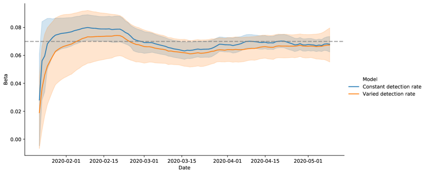
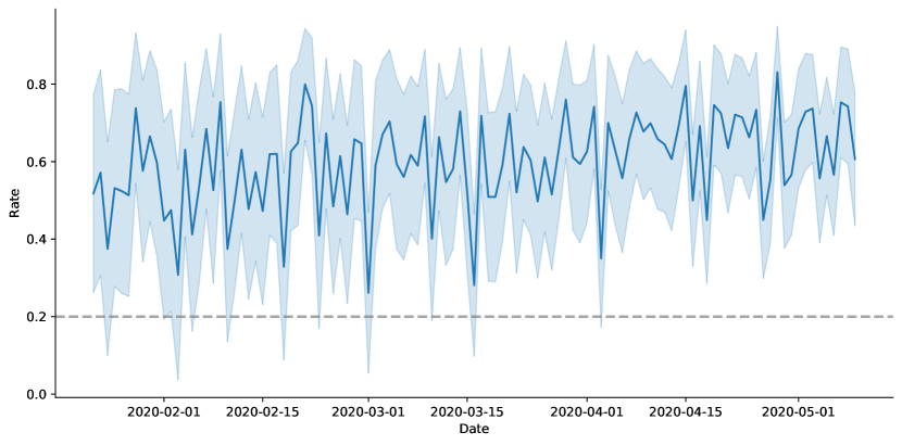
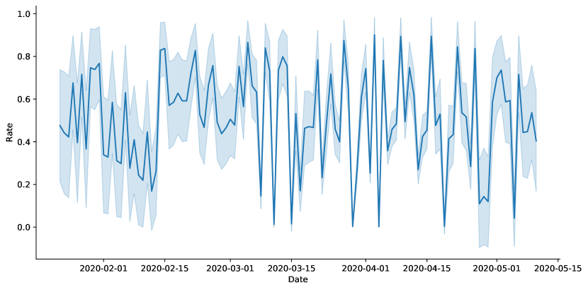
Fig. 1 and Fig. 2 show the estimated and for synthesized data using and . Fig 1 also shows the estimated by const-q model. the true is given to const-q model as data.
The results show that both models can estimate correctly, while completely fail to estimate . Estimated is biased to 1 and noisy. Therefore, our method cannot estimate the absolute level of the detection rate. However, the estimate of is still accurate so our method can be used to estimate . In fact, Fig. 3 and Fig. 5 shows that our model is robust against changing .
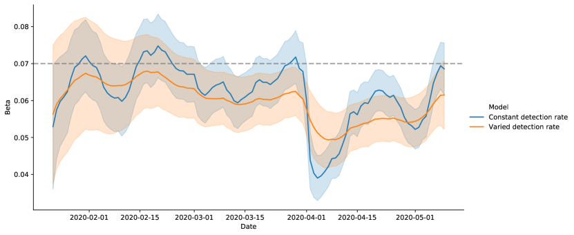
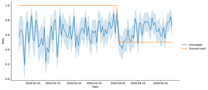
Fig. 3 and Fig. 4 show the estimated and for synthesized data using constant but changing which goes 1 to 0.8 in Apr. 1.
Fig 3 shows estimated by const-q model drops at April 1. Although the estimate by our model also drops around the same date, the drop is less significant. This indicates that allowing vary makes an estimated robust against a sudden change of .
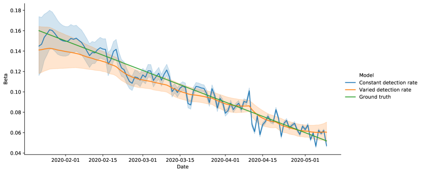
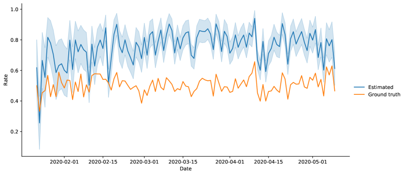
Fig. 5 and Fig 6 show the estimated and for synthesized data using linearly decreasing and noisy . Fig. 5 shows that our method is smooth while the estimate of const-q is noisy. Again, this shows that our model is more robust against changing . Further, Fig 6 indicates that while the estimated is biased toward 1, the short-term change coincides the ground truth. Therefore, the estimated is still useful to find a short-term shock to the detection rate.
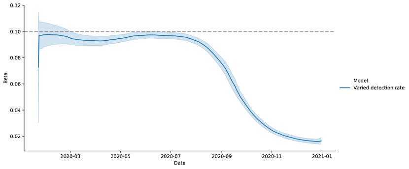
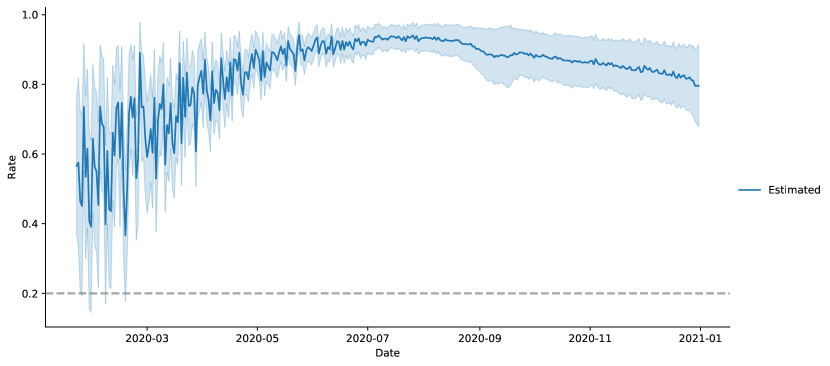
Fig. 7 and Fig. 8 show the estimate of and for data generated with constant and . Unlike Fig. 1 and Fig. 2, and time horizon are chosen so that most of population are infected in the end. The result shows that the estimate of becomes unreliable when the infection starts saturated. Therefore, our model is only useful for the case of a low infection rate. The estimated by const-q swings widely, therefore is omitted.
In summary, the estimate of , which is a key parameter for estimate , by our model is robust against sudden changes and noise in , even though the estimate of itself is unreliable. When the infection begins to saturate among population, the estimate of as well as becomes unreliable.
4.2. Analysis of Japan
Next, we present our analysis of Japanese data.
First, we applied three models, const, const-q and our model (varied-q) to Japanese data. For all parameters of all models, holds so convergence is excellent. Then two information criteria, PSIS-LOO-CV and WAIC are applied to const, const-q and varied-q. The results are shown in Table 1.
| Model | PSIS-LOO | DSE(PSIS-LOO) | WAIC | DSE(WAIC) |
|---|---|---|---|---|
| varied-q | 792.209 | 0 | 720.258 | 0 |
| const-q | 809.442 | 6.44946 | 730.481 | 3.76378 |
| const | 5056.46 | 809.672 | 5768.74 | 1042.7 |
Table 1 shows that our model, varied-q, is the best model. However, we need to be careful because the difference between const-q is not large. Further, there is a data point in which the Pareto-k for the importance weight distribution is larger than 0.7. Therefore, the model is not robust and influenced too much from small numbers of data points.
Keeping this in mind, we tentatively choose varied-q and we analyze the result of varied-q.
Fig. 9 shows an estimated for each day in Japan by varied-q.
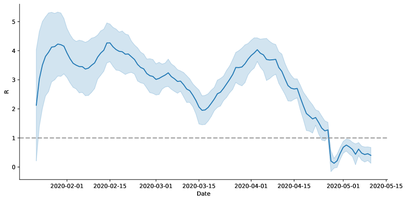
The first upward trend may not be very reliable because there is a few data for infection. The downward trend from the mid. February until the mid. March could be explained by public awareness and tracking effort of infection. After the mid. March, the tracking effort might be overwhelmed, thus created an upward trend until the beginning of April, when “the state of emergency” was declared to major urban areas. Since then, there was a downward trend, and now is below . Thus, currently the infection is shrinking.
4.3. Sensitivity analysis
Before going analysis of other countries, we analyze sensitivity of the result to prior distributions using Japanese data as an example.
Fig. 9 shows an estimated for each day in Japan by varied-q.
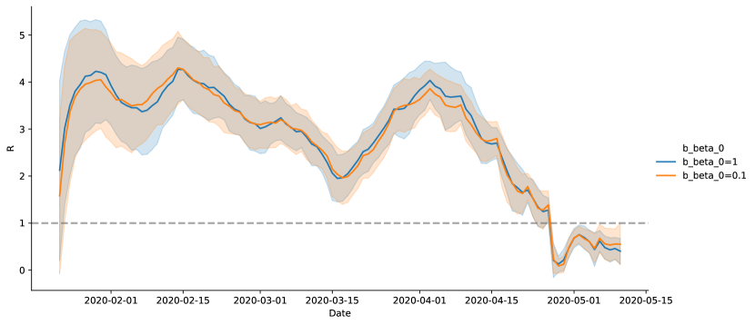
The blue line shows the estimate of based on the prior , which are used throughout in this paper. The orange line shows the estimate of based on the prior . There is no significant difference of estimates between two priors; therefore we can safely conclude that the effect of prior is small.
4.4. Comparison of Denmark and Sweden
Next, we compare Denmark and Sweden. These countries are economically and socially similar countries, but employed very different policies against COVID-19.
We applied the same procedure as Japan to data from two countries. All parameters are converged and information criteria favor varied-q model.
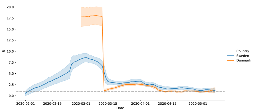
For Sweden, we only applied data from Mar 1. because the confirmed cases only appear in February 27. The estimated clearly shows that lock-down introduced March 13. was effective to put down . However, in Sweden, which did not employ lock-down, reduced gradually and now is almost same between Denmark and Sweden. This might suggest that lock-down is not very effective in long run but might also due to unfavorable conditions to Denmark, for example, higher population density.
4.5. Multi-national comparison
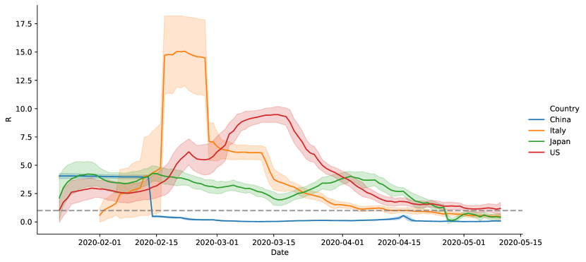
Fig. 13 shows daily estimate of of China, Italy, Japan and US. The same method as Japan was applied to the rest of countries and adequacy of varied-q model was verified. For Italy, we only apply data from March 1, 2020 because otherwise the parameter estimation did not converge. The same method was applied to Korea but the parameter estimation does not converge.
The results show that China, Italy, Japan, and the US are about to exit epidemic.
5. Future work
The method used in this paper has several limitations.
First, as experiment used simulation data revealed, our method cannot determine the true level of detection rate, nor its long-term trends. To find the true detection rate, we need different kind of data, such as excess mortality.
Second, our model uses a naive SIR model and does not consider incubation period and reporting delay. We can reconstruct the date of exposure by back projection, so it would be interesting apply our method to such data.
Acknowledgement
The author thanks to Kentaro Matsuura and the Tokyo.R Slack group for many suggestions and advice on Bayesian modeling. The author also thanks to Peter Turchin, from whose work the author’s work started.
References
- [1] Cleo Anastassopoulou, Lucia Russo, Athanasios Tsakris, and Constantinos Siettos. Data-based analysis, modelling and forecasting of the COVID-19 outbreak. Plos One, 15(3):e0230405, 2020.
- [2] Diego Caccavo. Chinese and Italian COVID-19 outbreaks can be correctly described by a modified SIRD model. medRxiv, page 2020.03.19.20039388, 2020.
- [3] Bob Carpenter, Andrew Gelman, Matthew D Hoffman, Daniel Lee, Ben Goodrich, Michael Betancourt, Marcus Brubaker, Jiqiang Guo, Peter Li, and Allen Riddell. Stan: A probabilistic programming language. Journal of statistical software, 76(1), 2017.
- [4] Seth Flaxman, Swapnil Mishra, Axel Gandy, Juliette T Unwin, Helen Coupland, Thomas A Mellan, Harrison Zhu, Tresnia Berah, Jeffrey W Eaton, Pablo N P Guzman, Nora Schmit, Lucia Cilloni, Kylie E C Ainslie, Marc Baguelin, Isobel Blake, Adhiratha Boonyasiri, Olivia Boyd, Lorenzo Cattarino, Constanze Ciavarella, Laura Cooper, Zulma Cucunubá, Gina Cuomo-Dannenburg, Amy Dighe, Bimandra Djaafara, Ilaria Dorigatti, Sabine Van Elsland, Rich Fitzjohn, Han Fu, Katy Gaythorpe, Lily Geidelberg, Nicholas Grassly, Will Green, Timothy Hallett, Arran Hamlet, Wes Hinsley, Ben Jeffrey, David Jorgensen, Edward Knock, Daniel Laydon, Gemma Nedjati-Gilani, Pierre Nouvellet, Kris Parag, Igor Siveroni, Hayley Thompson, Robert Verity, Erik Volz, Patrick Gt Walker, Caroline Walters, Haowei Wang, Yuanrong Wang, Oliver Watson, Xiaoyue Xi, Peter Winskill, Charles Whittaker, Azra Ghani, Christl A Donnelly, Steven Riley, Lucy C Okell, Michaela A C Vollmer, Neil M Ferguson, and Samir Bhatt. Estimating the number of infections and the impact of non-pharmaceutical interventions on COVID-19 in 11 European countries. Imperial College London, (March):1–35, 2020.
- [5] Ravin Kumar, Colin Carroll, Ari Hartikainen, and Osvaldo A. Martin. ArviZ a unified library for exploratory analysis of Bayesian models in Python. The Journal of Open Source Software, 2019.
- [6] Peter Turchin. Analyzing covid-19 data with sird models, 2020.
- [7] Aki Vehtari, Andrew Gelman, and Jonah Gabry. Practical Bayesian model evaluation using leave-one-out cross-validation and WAIC. Statistics and Computing, 27(5):1413–1432, 2017.
- [8] Sumio Watanabe. Asymptotic equivalence of bayes cross validation and widely applicable information criterion in singular learning theory. Journal of Machine Learning Research, 11(Dec):3571–3594, 2010.