An open tool for creating battery-electric vehicle time series from empirical data - emobpy

Abstract

There is substantial research interest in how future fleets of battery-electric vehicles will interact with the power sector. To this end, various types of energy models depend on meaningful input parameters, in particular time series of vehicle mobility, driving electricity consumption, grid availability, or grid electricity demand. As the availability of such data is highly limited, we introduce the open-source tool emobpy. Based on mobility statistics, physical properties of vehicles, and other customizable assumptions, it derives time series data that can readily be used in a wide range of model applications. For an illustration, we create and characterize $200$ battery-electric vehicle profiles for Germany. Depending on the hour of the day, a fleet of one million vehicles has a median grid availability between $5$ and $7$ gigawatts, as vehicles are parking most of the time. Four exemplary grid electricity demand time series illustrate the smoothing effect of balanced charging strategies.

1 Introduction

We introduce emobpy. It is an open-source python-based tool that creates profiles of battery-electric vehicles (BEV), based on empirical mobility statistics and customizable assumptions. We additionally provide a first application of the tool and create vehicle profiles based on representative German mobility data. An emobpy profile consists of four time series: (i) vehicle mobility containing the vehicle’s location and distance travelled, (ii) driving electricity consumption, specifying how much electricity is taken from the battery for driving; (iii) BEV grid availability, providing information whether and with which power rating a BEV is connected to the electricity grid at a certain point in time; and (iv) BEV grid electricity demand, specifying the actual charging electricity drawn from the grid, based on different charging strategies.

Such profiles are core input data for a wide range of model applications in energy, environmental, and economic studies on BEV. Technology developments as well as energy and climate policy measures drive the deployment of BEV in many countries [eia_2019]. Growing BEV fleets can have substantial impacts on the power sector. They increase the electric load, but may also provide temporal flexibility for integrating variable renewable energy sources and contribute to decarbonizing transportation [ipcc_2018]. Many model-based analyses investigate potential power sector interactions of future BEV fleets [Daina_2017a, mwasilu_2014, richardson_2013, Taljegard_2019] and thus depend on a meaningful representation of electric vehicles’ mobility patterns.

Yet such data are often not publicly available. In general, empirical data are scarce because BEV fleets are still small in most countries. And if respective time series are available, they are often specific to the conditions in which the data was collected and subject to data protection provisions. Past approaches make either stylized coarse assumptions [Kempton_2005], derive data from mobility statistics, but lack documentation, transparency or reproducibility [Fischer_2019, Kiviluoma_2011, Muratori_2018, robinson_2013, schaeuble_2017, schill_2015, Heinz_2018], or are idiosyncratic with respect to geographic characteristics or assumed driver behavior [Chen_2018, robinson_2013, Wolinetz_2018].

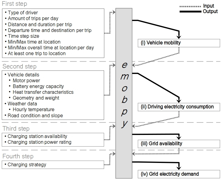
Figure 1: Inputs and outputs for emobpy and sequence of generating four types of time series. The boxes on the left-hand side show customizable input assumptions, the boxes on the right-hand side indicate the four types of time series.

Following [Daina_2017a], we argue that new models are needed to derive relevant time series in a transparent and flexible way. As a first step in this direction, the tools Vencopy [Wulff2020] and RAMP-mobility [LOMBARDI2019] recently emerged. To further fill this gap, we developed emobpy. Our tool takes empirical mobility statistics, physical properties of vehicles, and customizable assumptions as inputs and delivers BEV profiles as output. Figure 1 gives a stylized account. We first discuss the outputs, then the required inputs.

Four output time series constitute one BEV profile. These profiles have a customizable length and resolution. A handy format for many applications is all hours of one year. But also other formats are possible by discretion of the researcher. Likewise, the researcher can choose how many profiles she wants to create.

The time series of vehicle mobility (i) contains the location of the vehicle at each time step and the time steps during which the vehicle is driving with information of the distance traveled. The driving electricity consumption time series (ii) provides information on how much electricity the vehicle consumes for driving in each time step. The time series of (iii) grid availability provides information whether a vehicle is connected to the electricity grid in a time step and if so, with what power rating for charging or discharging. The time series of grid electricity demand (iv) provides information on how much electricity a vehicle demands from the electricity grid in a time step. Time series (i), (ii) and (iii) are core inputs for models that endogenously determine the timing of charging (and, potentially, discharging to the grid); the time series (iv) are core inputs for models that do not endogenously determine the grid interactions of BEV, but use exogenous input data for this.

The required input data for the time series of vehicle mobility (i) are the relative frequencies of different driver types, e.g., commuters, of the number of trips per day, of the destination, distance and duration of trips, and of the departure hours. Such information can often be derived from national mobility statistics. If required or desired, a researcher can also make up own assumptions or resort to the pre-set values from German mobility statistics. emobpy makes sure that the resulting time series are feasible and consistent. To this end, a minimum and maximum number of hours at specific locations can specified, and it is assumed that the last trip of a day heads home. With a Monte Carlo approach, emobpy ensures variability across profiles.

Based on the vehicle mobility time series, the driving electricity consumption (ii) time series is derived. This requires further input data, such as information on nominal motor power, curb weight, drag coefficient, and dimensions, which the tool includes for several current BEV models. Ambient temperature is also a significant parameter that affects the consumption of BEV [Brown_2018, Fischer_2019]. For that reason, emobpy is endowed with a database of hourly temperature for European countries with a registry of the last 17 years. Additionally, the vehicle cabin insulation characteristics are required; this data is not widely available and thus assumed independently of the BEV models database. Driving cycles are also important input parameters that are used to simulate every individual trip. The model includes two driving cycles, Worldwide Harmonized Light Vehicles Test Cycle (WLTC) and Environmental Protection Agency (EPA). This input data is already provided within the tool, and the user can select a particular BEV model, country weather and driving cycle. Additionally, emobpy also allows providing user-defined custom data.

The required input data for the grid availability time series (iii) is the driving electricity consumption time series (ii). Further, data or assumptions on the power rating of charging stations at different generic locations as well as their availability probabilities are needed. Variability across profiles is, again, introduced through a Monte Carlo approach, while emobpy makes sure that the time series (iii) is consistent within each profile .

The required input data for the grid electricity demand time series (iv) includes the created time series on driving electricity consumption (ii) and grid availability (iii). Additionally, users can choose a charging strategy, such as immediate full charging or night-time charging, or make customary assumptions.

2 Results

2.1 Application to Germany: parameterization and setup

For a first application of emobpy, we draw on the comprehensive German mobility survey Mobilität in Deutschland [MID_2017, Mobility in Germany,]. The survey features mobility data relating to different types of households, vehicles, individuals, and trips. In this application, we make three general assumptions: first, we assume that individuals with access to a vehicle carry out all their trips with the same vehicle; second, we assume that future BEV drivers have similar mobility patterns as current conventional drivers covered by the underlying mobility statistics; and third, for simplicity and tractability, we assume that there are only four BEV models: Hyundai Kona, Renault Zoe, Tesla Model 3 and Volkswagen ID.3. These models had the largest market shares in Germany by the time of writing. Again, all of these pre-set assumptions can easily be modified in emobpy.

We generate $50$ profiles for each BEV model, i.e., $200$ BEV profiles overall, each consisting of four time series. We focus on two types of drivers: commuters ($62$% of all drivers) and non-commuters ($38$% of all drivers). For commuters, we further differentiate between full-time and part-time employees, with a split of $78$ to $22$% [OCDE_2018]. We exclude commuting students, apprentices, and trainees, who represent only a small share of all commuters in the initial dataset. The amount of trips per day varies between $0$ - $5$ with different probabilities for weekdays and weekend days (Table 2.1).

Table 1: Probability distributions (given in %) for the amount of trips per day by days of the week