An obscured AGN population hidden in the VIPERS galaxies: identification through spectral energy distribution decomposition

Abstract

The detection of X-ray emission constitutes a reliable and efficient tool for the selection of Active Galactic Nuclei (AGNs), although it may be biased against the most heavily absorbed AGNs. Simple mid-IR broad-band selection criteria identify a large number of luminous and absorbed AGNs, yet again host contamination could lead to non-uniform and incomplete samples. Spectral Energy Distribution (SED) decomposition is able to decouple the emission from the AGN versus that from star-forming regions, revealing weaker AGN components. We aim to identify the obscured AGN population in the VIPERS survey in the CFHTLS W1 field through SED modelling. We construct SEDs for 6,860 sources and identify 160 AGNs at a high confidence level using a Bayesian approach. Using optical spectroscopy, we confirm the nature of $\sim$85% of the AGNs. Our AGN sample is highly complete ($\sim$92%) compared to mid-IR colour selected AGNs, including a significant number of galaxy-dominated systems with lower luminosities. In addition to the lack of X-ray emission (80%), the SED fitting results suggest that the majority of the sources are obscured. We use a number of diagnostic criteria in the optical, infrared and X-ray regime to verify these results. Interestingly, only 35% of the most luminous mid-IR selected AGNs have X-ray counterparts suggesting strong absorption. Our work emphasizes the importance of using SED decomposition techniques to select a population of type II AGNs, which may remain undetected by either X-ray or IR colour surveys.

1 Introduction

Recent studies show that almost all galaxies in the Local Universe host a super-massive black hole (SMBH) in their centre (Magorrian et al., 1998; Kormendy & Kennicutt, 2004; Filippenko & Ho, 2003; Barth et al., 2004; Greene & Ho, 2004, 2007; Dong et al., 2007; Greene et al., 2008). Their mass ranges between $10^{5}$ and $10^{10}$ solar masses. When matter from the galaxies starts to accrete into the SMBH, an enormous amount of energy is released across the electromagnetic spectrum (from radio emission up to X- and $\gamma$- rays). This constitutes the characteristic signature of Active Galactic Nuclei (AGNs). In many cases, the power of a single AGN with a similar size to our Solar System is higher than the power emitted by the stellar population of its host galaxy. The detection and study of AGNs is one of the most active fields of extra-galactic astrophysics today. Their demographics (e.g. space density), their distribution on the cosmic web (e.g. two-point auto-correlation function) and their physical properties (e.g. luminosity, black hole mass, accretion rate, absorption) play an important role in understanding the evolutionary models of black holes and whether AGN affect their host galaxy properties (e.g. star formation rate). Recent studies suggest a close interaction between the creation and evolution of galaxies and that of SMBHs (e.g. Silk & Rees, 1998; Granato et al., 2004; Di Matteo et al., 2005; Croton, 2006; Hopkins et al., 2006, 2008; Menci et al., 2008), though the physical processes governing this relationship are not yet fully understood.

To investigate any parallel evolution between galaxies and AGN, as well as to examine whether and how AGN feedback affects the evolution of galaxies, observations in infrared (IR), optical wavelengths and X-rays are required (Hopkins et al., 2006; Bower et al., 2006). The properties of galaxies hosting a black hole can be studied using optical and near-IR observations, while the absorbed AGN properties can be investigated in both X-rays and the mid-IR regime (Hickox & Alexander, 2018, and references therein). When the radiation of AGN dominates, X-ray emission is capable of penetrating large amounts of dust and gas without being absorbed. Consequently, the detection of X-rays is one of the most efficient methods of identifying AGNs and is essentially independent of absorption (Luo et al., 2008). However, even hard X-rays can be absorbed in the presence of huge amounts of dust and gas (Gilli et al., 2007; Fiore et al., 2008; Treister et al., 2009; Akylas et al., 2012).

Mid-IR selection techniques offer a powerful tool to separate AGNs from stars and galaxies. This is achieved by separating the (approximately) power law AGN spectrum from the black body stellar spectrum of galaxies. Thus, another way of detecting AGNs is through mid-IR observations, which has the advantage of being affected less by extinction. Mid-IR broad-band colour selection criteria have been proven extremely useful in revealing the presence of an AGN (Lacy et al., 2007; Stern et al., 2012; Mateos et al., 2012; Donley et al., 2012; Assef et al., 2013) based on observations made by the Wide-field Infrared Survey Explorer (WISE; Wright et al., 2010) and the Spitzer Space telescope (Werner et al., 2004). Furthermore, many studies used the IR selection criteria in combination with X-ray or optical photometric and spectroscopic data to uncover absorbed AGN (e.g. Rovilos et al., 2014; Hainline et al., 2014; Assef et al., 2015; Hviding et al., 2018; Glikman et al., 2019). However, IR selection techniques are biased against low-luminosity AGNs (Barmby et al., 2006; Georgantopoulos et al., 2008). SED decomposition can alleviate this problem by utilizing large wavelength range and properly disentangle accretion from star formation (e.g. Ciesla et al., 2015). SED decomposition can therefore provide a complementary tool to the X-ray and IR selection techniques, revealing weaker AGN systems with lower luminosities by reliably quantifying the host galaxy contribution to mid-IR colours.

This work focuses on selecting AGNs through SED modelling and fitting techniques in a sample of galaxies from the VIPERS survey (Guzzo, L. et al., 2014; Garilli, B. et al., 2014). We aim to find an AGN population with intermediate/high obscuration, which would be missed from current X-ray surveys and simple mid-IR colour cuts. The optical, near-IR and mid-IR data used for the SEDs along with ancillary data (spectroscopic data, X-ray catalogues, etc.) are presented in Section 2, while in Section 3, we describe the methods we used to construct and model the SEDs and also a Bayesian approach to select AGNs. In Section 4, we explore the optical spectra, demonstrate the properties of the SED selected AGNs in the mid-IR and X-ray regimes and we focus on the obscuration of these sources by applying different diagnostic tests. In Section 5, we discuss these properties along with the differences between SED, mid-IR and X-ray selected AGNs, while Section 6 presents the summary of the results and conclusions. Throughout the paper, we assumed a $\Lambda$CDM cosmology with H_o=75 km s^-1 Mpc^-1, $\Omega$_M=0.3 and $\Omega$_$\Lambda$=0.7.

2 Data

The selection of obscured AGNs through SED fitting analysis requires secure redshifts and available optical and IR photometry for the SED construction. For that purpose, we used data from the VIMOS Public Extragalactic Redshift Survey (VIPERS) in the Canada-France-Hawaii Legacy Survey (CFHTLS) W1 field that contains rich multi-wavelength data from X-rays to the mid-IR bands.

2.1 VIPERS

The VIPERS survey used the VIsible MultiObject Spectrograph (Le Fèvre, O. et al., 2013, VIMOS) to perform deep optical spectroscopy within the CFHTLS W1 field. Follow-up spectroscopic targets were selected to the magnitude limit i’$=22.5$ from the CFHTLS catalogues (Guzzo, L. et al., 2014), while an optical colour pre-selection excluded galaxies at z$<0.5$ (Le Fèvre et al., 2013). Comparing with a sample of VVDS-Deep and VVDS-Wide surveys, the selection criteria yielded $100\%$ completeness for z$>0.6$ (Fig.4, Scodeggio et al., 2018). In our analysis, we use the Public Data Release 2 (PDR-2, Scodeggio et al., 2018) of the VIPERS survey, which consists of 86,775 galaxies with available spectra and their corresponding optical photometric data in the u, g, r, i and z bands from the CFHTLS T0007 data release (Hudelot et al., 2012). Each spectrum is assigned a quality flag. In this work, we use sources with flags higher than 2 (confidence level of redshift measurement higher than 90% based on more than one spectral features) that are considered as the most reliable (Garilli, B. et al., 2014; Scodeggio et al., 2018). In total, 45,180 galaxies meet this criterion within $0.5<z<1.2$.

2.2 VISTA-VHS

The VISTA Hemisphere Survey (VHS, McMahon et al., 2013) is one of the six large surveys that are coordinated by the Visible and Infrared Survey Telescope for Astronomy (VISTA, Emerson et al., 2006) to observe the entire sky in the southern hemisphere, covering 20,000 sq. degrees. The data used in this work are from the Data Release 6 that produced by the VISTA Science Archive (VSA). VSA handles all the data products generated by the VISTA Infrared CAMera (VIRCAM). The depth of the VHS observations is higher than other near infrared surveys, such as UKIDSS-LAS (Lawrence et al., 2007), 2MASS (Skrutskie et al., 2006) or DENIS (Epchtein et al., 1994), and the magnitude limits are 20.6, 19.8 and 18.5 mag (Vega) for the J, H and Ks band, respectively.

2.3 AIIWISE

The usage of mid-IR photometry, in our analysis, is twofold: First, its inclusion in the SED fitting process allow us to identify AGN candidates (see Section 3). Second, mid-IR photometry has been proven very efficient in detecting AGNs, since it is less affected by extinction. We, thus, compare our SED derived AGN candidates with those selected by IR colours (see Section 4). Launched by NASA, WISE mapped the whole sky in the mid-IR regime with its four band-passes: W1=3.4 $\mu$m, W2=4.6 $\mu$m, W3=12 $\mu$m and W4=22$\mu$m and reached 5$\sigma$ depths of 16.5, 15.5, 11.2, and 7.9 mag in Vega system, respectively. The AllWISE source catalogue (Cutri & et al., 2013) consists of more than 700 million objects with signal-to-noise ratio higher than 5 in at least one band in the combined images.

2.4 XMM-XXL

XMM-XXL field (Pierre et al., 2017) covers an area of $\sim$50 deg² with an exposure time of about 10 ks per XMM-Newton pointing. The survey is split into two approximately equal fields. In the analysis, we use data from the equatorial sub-region of the field (XMM-XXL-North; XXL-N) that overlaps with the CFHTLS W1 field and covers an area of about 25 deg². We make use of the most recent X-ray catalogue of Chiappetti et al. (2018), which consists of 14,168 X-ray sources in the northern XMM-XXL field.

2.5 Final sample

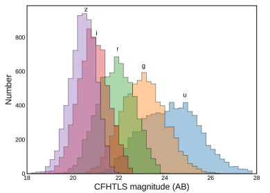
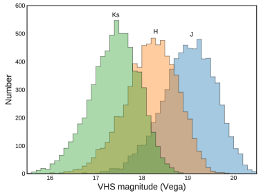
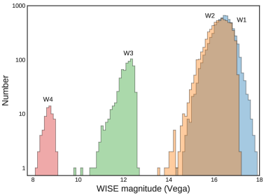
Figure 1: The magnitude distributions of our initial sample of 6,860 sources for the CFHTLS optical bands u, g, r, i and z (top), the VHS near-IR bands J, H and Ks (middle) and the WISE mid-IR bands W1, W2, W3 and W4 in Vega system (bottom) with signal-to-noise ratio higher than three.

The VIPERS catalogue with spectroscopic redshfits and optical photometry was cross-matched with the list of mid-IR AllWISE and the near-IR VHS sources at the same time using the xmatch tool from the astromatch package that uses different statistical methods for cross-matching of astronomical catalogues. This tool matches symmetrically a set of catalogues and gives the Bayesian probabilities of the associations or non-associations (Pineau et al., 2017). To properly perform xmatch, all the cross-matched catalogues must cover the same footprint. As AllWISE is an all-sky survey and the VHS data cover the entire VIPERS field, we selected only the IR sources that lie in the footprint of the VIPERS survey. After the cross-match with xmatch, we kept only sources with a high probability of association (>68%). When one source was associated with several counterparts, we selected the association with the highest probability. We then filtered out sources with signal-to-noise ratio lower than three in the near-IR and mid-IR bands to better constrain the SED fitting in the IR regime. The resulted catalogue of 6,860 sources was used as the parent sample (hereafter as VIPERS sample).

In Figure 1, we show the optical, near-IR and mid-IR (from top to bottom) magnitude distributions of our final sources with signal-to-noise ratio higher than three, while in Figure 2 we present their corresponding redshifts (blue histogram). All the mid-IR (WISE) magnitudes were measured with profile-fitting photometry, since all the sources are point-like (ext_flg=0) in the mid-IR images, which may be due to the low angular resolution of WISE telescope (e.g. $\sim$6.1" for W1 band). The shape of the magnitude distributions in the optical and near-IR bands (Fig. 1) is Gaussian-like, while the mean magnitude value becomes brighter from the u band (24.3 mag) to Ks band (17.4 mag). This is consistent with the expected magnitudes of the underlying host galaxy SEDs. Finally in the mid-IR bands, the number of W3 and W4 detections is lower compared to the shorter-wavelength mid-IR bands. This could be attributed to the fact that the AllWISE W3 and W4 bands have much lower sensitivity compared to W1 and W2 bands.

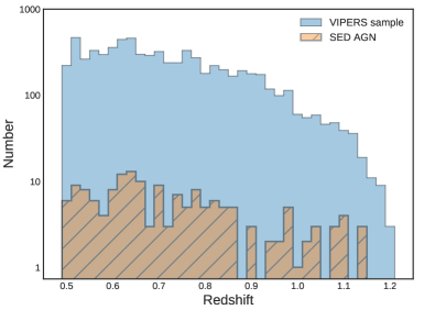
Figure 2: Redshift distribution for all sources in the initial sample (blue) and for the 160 high-confidence SED selected AGNs (orange-hatched).

3 Analysis

In this Section, we present the templates and parameter space used to fit the SEDs of the sources and the Bayesian methodology applied to select AGNs among these sources. We performed SED analysis using all the available optical (CFHTLS), near-IR (VHS) and mid-IR photometry (WISE), using X-CIGALE (Yang et al., 2020) that is the latest version of the Code Investigating GALaxy Emission (CIGALE, Noll et al., 2009; Ciesla et al., 2015; Boquien et al., 2019). This allows us to estimate the physical parameters of the sources. In particular, we are interested in the fraction of the IR luminosity originating from the AGN to the total IR luminosity of the galaxy, which is used as a proxy of the AGN activity (Ciesla et al., 2015). The SEDs were first fitted with a) a galaxy template and b) a galaxy plus an AGN component. For each case, we obtained the best-fitting solution provided by X-CIGALE, and used the Bayesian Information Crirerion (BIC, Schwarz, 1978) to quantify which template (galaxy/galaxy+AGN) provides the best fit for each source and the highest probability to host an AGN. We describe the analysis steps in detail below.

Table 1: Models and the values for their free parameters used by X-CIGALE for the SED fitting of our initial sample (6,860 sources).

Parameter		Value
Star formation history: double-exponentially-decreasing ($\tau$-dec) model
Age of the main stellar population		0.5, 1.0, 3.0, 5.0, 7.0, 9.0, 11.0, 13.0
$\tau_{main}$		0.1, 0.5, 1.0, 3.0, 5.0, 10.0, 20.0
$age_{burst}$		0.1, 0.2, 0.4, 0.5
Stellar population synthesis model
Single Stellar Population Library		Bruzual & Charlot (2003)
Initial Mass Function		Salpeter
Metallicity		0.02 (Solar)
Nebular emission
Ionization parameter ($logU$)		-2.0
Fraction of Lyman continuum escaping the galaxy ($f_{esc}$)		0.0
Fraction of Lyman continuum absorbed by dust ($f_{dust}$)		0.0
Line width in km/s		300.0
Dust attenuation: Calzetti et al. (2000)
Colour excess of stellar continuum light for young stars E(B-V)		0.05, 0.1, 0.2, 0.3, 0.35, 0.4, 0.5, 0.6
Reduction factor for the E(B-V) of the old stars compared to the young ones		0.44
Dust template: Dale et al. (2014)
IR power-law slope		2.0
AGN models from Fritz et al. (2006)
Ratio between outer and inner radius of the torus ($r_{ratio}$)		60.0
Optical depth at 9.7 $\mu$m ($\tau$)		0.1, 1.0, 6.0, 10.0
Parameter linked to the radial dust distribution in the torus ($\beta$)		-0.5
Parameter linked to the angular dust distribution in the torus ($\gamma$)		4.0
Angular opening angle of the torus ($\theta$)		100.0
Angle with line of sight ($\psi$)		0.001, 50.100, 89.990
AGN fraction		0.1, 0.2, 0.3, 0.5, 0.7, 0.9
Extinction in polar direction, E(B-V)		0.0, 0.05, 0.1, 0.15, 0.2, 0.3, 1.0
Emissivity of the polar dust		1.6
Temperature of the polar dust (K)		100.0

• Note. – $\tau_{main}$ is the e-folding time of the main stellar population model in Gyr, age is the age of the main stellar population in the galaxy in Gyr (the precision is 1 Myr), and $age_{burst}$ is the age of the late burst in Gyr (the precision is 1 Myr). $\beta$ and $\gamma$ are the parameters used to define the law for the spatial behaviour of the torus density. The functional form of the latter is $\rho(r,\theta)\propto r\beta e^{-\gamma|cos\theta|}$, where r and $\theta$ are the radial distance and the polar distance, respectively. $\theta$ is the opening angle and $\psi$ the viewing angle of the torus. Type-2 AGNs have $\psi$ = 0.001 and Type-1 AGNs have $\psi$ = 89.990, while values equal to $\psi$ = 50.100 are for intermediate type of AGN. The extinction in polar direction, E(B-V), included in the AGN module, accounts for the possible extincion in type-1 AGN, due to polar dust. The AGN fraction is measured as the AGN emission relative to IR luminosity (1–1000 $\mu$m).

The X-CIGALE algorithm fits the observational multi-wavelength data with a grid of theoretical models and returns the best-fitted values for the physical parameters. The results are based on the energy balance, i.e., the energy absorbed by dust in UV/optical is re-emitted after heating at longer wavelengths, such as the mid-IR and far-IR. In this work, we built a grid of models including different stellar populations, dust attenuation properties, dust emission, star formation history and AGN emission. In particular, the models and the parameter space covered by these components are described below:

1. To convolve the star formation histories of our sample, we used the double-exponentially-decreasing model (2$\tau$-dec). This model, provides the best stellar mass and star formation rates of the sources, at the expense of unrealistic galaxy ages (Ciesla et al., 2015). Using a different model, e.g., 1$\tau$-dec, delayed SFR, does not affect our measurements, as shown in Mountrichas et al. (2019).

2. For the simple stellar population, we used the synthesis models of Bruzual & Charlot (2003), assuming the Initial Mass Function by Salpeter. We adopted a constant, solar metallicity of Z = 0.02, and a separation age between the young and the old stellar populations within the range of 1.5-1000 Myrs. A constant metallicity for all sources prevents long time consuming calculations, but also it does not affect significantly the shape of the SEDs compared to the observed ones and the derived properties (Yuan et al., 2018; Hunt et al., 2019).

3. For the attenuation due to absorption and scatter of the stellar and nebular emission by interstellar dust, we utilized the attenuation law by Calzetti et al. (2000).

4. The emission by dust in the IR regime was modelled by the semi-empirical Dale et al. (2014) templates. The parameter that describes them is the power-law slope of the dust mass distribution over heating intensity, $\alpha$. These templates are strongly correlated to the adopted attenuation models through the dust luminosity that is the outcome of the energy balance that X-CIGALE is based on.

5. The AGN emission was modelled using the Fritz et al. (2006) template that includes both the emission from the central AGN and also the re-emitted radiation from the dusty torus heated by the central engine at longer wavelengths. Additionally, this latest version of the X-CIGALE code introduces polar-dust extinction to account for the possible extinction in type-1 AGN (Yang et al., 2020).

Table 1 presents the models and the values of their free parameters, used in the fitting process.

Table 2: Explanation of Bayes Factor and $\Delta$BIC values according to Kass & Raftery (1995) and selection of high-confidence SED AGNs compared to mid-IR and X-ray selected samples.

$\Delta$BIC	BF	Evidence in favor	AGN Probability	Number of	mid-IR	X-ray	X-ray & mid-IR
(2*log(BF))		of model m	(%)	SEDs (6,860)	AGN (52/35)	AGN (116)	AGN (17/14)
>10	>150	very strong	0.08	2,346	0/0	5	0/0
(6-10)	(3,20)	strong	2.50	2,053	1/0	29	0/0
(2-6)	(1,3)	little	11.35	1,894	5/3	40	2/2
(-2-2)	(<1)	equal for both	43.00	407	2/0	8	0/0
(-6,-2)	(3,20)	little	84.30	87	7/2	6	1/0
(-10,-6)	(20,150)	strong	97.62	17	7/5	4	3/2
<-10	>150	very strong	99.89	56	30/25	24	11/10
<-2	>3	strong	91.21	160	44/32	34	15/12

• Note. – For positive values of 2log(BF) the best model, m, is assumed to be this with only galaxy templates, while for negative values m represents the model when an AGN component is included. Thus, the evidence in each case refers to model m. The AGN probabilities are the average of each bin and refer to the model with AGN templates: high values indicate AGN activity. The number of SEDs refers to the number of sources in each $\Delta$BIC bin. The last three columns give the number of mid-IR, X-ray and both mid-IR and X-ray selected AGNs in these bins. In mid-IR AGN and the last columns, the two numbers correspond to selection criteria of Assef et al. (2013) with reliability of 75% and 90%, respectively. The last row corresponds to our AGN selection criteria with $\Delta$BIC$<-2$.

In Bayesian statistics, the choice of the model that fits best to the data is achieved through the Bayes Factor, BF. In Appendix A, we describe the procedure of calculating and evaluating the BF. The BF requires the calculation of the posteriori and the posteriori complementary probabilities. Alternative methods are required when the BF is calculated with not enough information for the a priori probabilities. Information Criteria, such as the Akaike Information Criterion (Akaike, 1974, AIC) or the Bayesian Information criterion (Schwarz, 1978, BIC), are applied, since they are capable of calculating an approximation of the BF in the absence of priori distributions. This is achieved, by taking into account the complexity of the models, in addition to the goodness of fit. In this work, we used BIC, since it evaluates the true model among all possible and alternative hypotheses, while it is more conservative in the parameter impact on the selection compared to AIC. It favors models with small number of parameters, while by increasing the parameter space, it penalizes more the model. The values of BIC for a model are given by:

$$BIC=-2*ln(L)+2*p*ln(N),$$ (1)

where p and N are the number of parameters and the number of observations, respectively, while L is the maximum likelihood of the model. To compare two models and select the best one, we calculate the difference of the information of the two models:

$$\Delta BIC=-2*ln(L_{1}/L_{2})-(p_{2}-p_{1})*ln(N),$$ (2)

where the first term of this equation gives the ratio of the likelihoods of the two models and (p₂-p₁) is the difference of the parameters used in each model. It can be shown that the difference in BIC values for two models, $\Delta$BIC, are related to BF, and in this case the latter can be calculated approximately by:

$$BF=exp(-\Delta BIC/2).$$ (3)

We further consider the Schwarz weights (Burnham & Anderson, 2002):

$$weight=\frac{exp(-\Delta BIC_{j}/2)}{\sum_{n=1}^{2}exp(-\Delta BIC_{n}/2)}.$$ (4)

These weights indicate the relative preference between two candidate models (n=1,2) and also provide a method to combine a parameter when using multiple model averaging. In other words, they express a probability that favours one model (in this case j) against the other. In Table 2, we give the interpretation for each value of $\Delta$BIC and we select the best model according to $\Delta$BIC values and the posteriori probability of each model.

4 Results

4.1 SED selected AGNs

To identify AGN candidates, we constructed and modelled the SEDs of all the 6,860 sources in the VIPERS sample. Each SED was fitted twice. In the first run, we used only galaxy model templates. In the second run, we used both galaxy and AGN templates. For each case, we obtained the best fitting model and we calculated the BIC values (Eq. 1). Based on the difference, $\Delta$BIC (Eq. 2), and its interpretation (Table 2), we classified the sources into samples with different evidence ratio (or AGN probability). Following Del Moro et al. (2016), we adopted a threshold of $\Delta$BIC$<-2$ to select AGN candidates. This results to 160 galaxies ($\sim$2.3% of the initial sample) with probabilities hosting an AGN higher than 73% (the mean value is equal to 91.20%) and evidence that favors the model when including the AGN templates. These sources also have lower values of the reduced $\chi^{2}$ in the model fitting when adding an AGN component. Figure 3 shows the $\Delta$BIC distribution for the VIPERS sample (blue histogram). The vertical dashed line denotes the threshold used in this work.

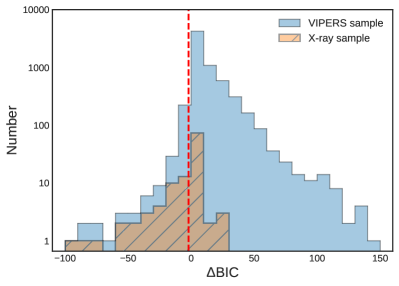
Figure 3: The distribution of $\Delta$BIC for the VIPERS sample (blue). The orange-hatched histogram represents the distribution only for the X-ray sample. The vertical dashed line represents the threshold used in this work adopted by Del Moro et al. (2017) corresponding to evidence that favors the model when including the AGN template.

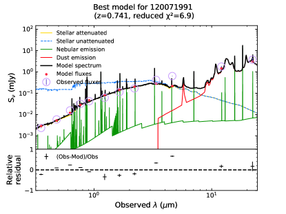
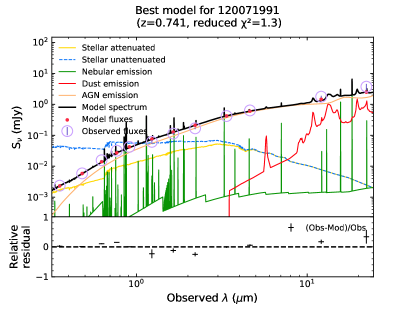
Figure 4: SED fitting example of a source classified as AGN with probability 99.99%. The upper and lower SEDs correspond to models without and with AGN templates, respectively. The dust emission is plotted in red, the AGN component in green, the attenuated (unattenuated) stellar component is shown with the yellow (blue) solid (dashed) line, while the orange lines shows the nebular emission. The total flux is represented with black colour. Below each SED, we plot the relative residual fluxes versus the wavelength.

In Figure 4, we present the SEDs with and without AGN templates (lower and upper panels, respectively) for a source classified as AGN, with probability of 99.99%. When an AGN component is added to the fitting process, the fit is significantly improved and the relative residual fluxes are minimized, as shown at the bottom of each panel. In Table 4 in the Appendix, we list the properties of the 160 SED selected AGNs, while Figure 2 shows their redshift distribution (orange-hatched histogram). We, further, explored (Appendix C) whether the availability of photometry at different wavelengths affects the AGN selection method. Our analysis showed that near-IR photometry (in addition to optical and mid-IR) is crucial for the reliability of the methodology. However, absence of far-IR or mid-IR photometry at longer wavelengths (W3, W4 photometric bands) does not affect the selection of AGN candidates.

The inclination angle, $\psi$, is defined as the angle between the equatorial AGN axis and the line of sight. Although, (X-) CIGALE cannot constrain the exact value of $\psi$ this parameter can be used as an indication for classifying AGN into type-1 and type-2 (Ciesla et al., 2015; Yang et al., 2020). Specifically, $\psi=90^{o}$ denotes type-1 AGN, whereas $\psi\leq 50^{o}$ indicates intermediate or type-2 AGN. According to the SED fitting results, $71\%$ of the sources have inclination angle values $\leq 50^{o}$. In particular, 46/160 (29%) and 81/160 (51%) have $\psi=50^{o}$ and $\psi=0^{o}$, respectively. Thus, the vast majority (70%) of our AGN candidates seem to present some level of obscuration. To further investigate the nature of the sources, in the next subsections we examine their optical spectra, their X-ray and mid-IR properties and we apply different obscuration diagnostics using optical and IR colours.

4.2 X-ray detections and upper limits

In this section, we explore the X-ray properties of our 160 SED selected AGN. We use the most recent available X-ray catalogue to search for counterparts, while for non detections we derive upper limits by constructing the X-ray mosaic using all available images in the field. Out of 14,168 X-ray sources in the northern XMM-XXL field (Chiappetti et al., 2018), 10,029 sources ($\sim$70%) fall inside the field of view of the VIPERS pointings. Cross-matching this sample with the whole VIPERS catalogue using the xmatch software (see Section 2.5), there are 4,736 sources with high probability of association (68%). 359 of them have good quality spectroscopic redshifts (see Section 2.5) and are within the redshift range used in this study $(0.5<z<1.2)$. $116/359$ have optical, near-IR and mid-IR counterparts with a signal-to-noise ratio greater than three in the W1 and W2 WISE bands. The $\Delta$BIC distribution of the 116 X-ray sources is shown in Figure 3. Out of these, 34 sources ($\sim$30%) are also SED selected AGNs ($\Delta$BIC$>$-2). This means that the remaining 70% is not selected with the SED fitting technique. These sources should be AGNs with small amount of dust in their torus (or dust-free) and/or low IR contribution to the total of their hosts making them difficult to identify in the mid-IR wavelengths. We examine the nature of the latter in the next sections.

For the 126 SED selected AGNs not detected in X-rays, we derived the upper limits in the soft [0.5-2 keV] and hard [2-8 keV] bands. First, we constructed the mosaics taking into account all the publicly available XMM-Newton observations (Jansen et al., 2001) covering the XMM-XXL northern field. The detailed imaging procedure is described in Ruiz & Georgakakis (in prep.). Briefly, we retrieved and processed the overlapping observations in the field from all detectors by following the standard data reduction tasks of the XMM-Newton Scientific Analysis Software (Gabriel et al., 2004, SAS) and accounting for all the latest calibration files. EPIC-pn (Strüder et al., 2001) and both MOS-1 and MOS-2 (Turner et al., 2001) detectors were operated in full frame mode using the thin filter. The event files from all detectors were cleaned from hot pixels/columns and pixels at the edges of the cameras and were screened to remove high particle background and soft proton flares by setting FLAG=0 and selecting pn and MOS single events with 0<PATTERN<4 and PATTERN<=12, respectively. In a similar way, we built the combined mosaic with the exposure maps. The background mosaics were produced by masking the areas around the X-ray detections.

For the upper limits, we extracted the total counts around the sources within a circular region of radius equal to 15". For the background, we used a circular region centered on the target position with a radius of 30" and we normalized this to the area of the sources. Then, we used a Bayesian approach of 99.7% confidence level to derive upper limits (Kraft et al., 1991). To find the final count rates, we divided the upper limits with the exposure time and the encircled energy fraction ($eef$): $count\,rate=upper\,limit/eef/exposure\,time$. The exposure time was taken as the average value of the pixels in a circular region of 15", while we adopted $eef$=0.7 that corresponds to the radius used for the sources extraction counts. The count rates were converted to fluxes, using an energy conversion factor ($ecf$) calculated for each band. For the $ecf$ calculation, we used the webbPIMMS site by assuming a power-law model with photon index of $\Gamma=1.7$ (Nandra et al., 2005; Tozzi et al., 2006) and galactic absorption $N_{H}=2.6*10^{20}$cm^-2. We calculated separately the $ecf$ for the pn and MOS thin filters and we took the average of them all. The final $ecf$ used are equal to $2.58\times 10^{11}$ and $6.82\times 10^{10}$ ergs photon^-1 for the soft and hard band, respectively. The luminosities were calculated using the following equation:

$$L_{X}=4*\pi*D_{L}^{2}*F_{X}*(1+z)^{\Gamma-2},$$ (5)

where L_X and F_X are the flux and luminosity in the hard band, respectively, D_L is the luminosity distance, z is the redshift and $\Gamma$ is the photon index (Alexander et al., 2003; Xue et al., 2011). The units of L_X are given in erg s^-1.

4.3 Mid-IR selected AGNs

In addition to studying their X-ray properties, we explore whether the 160 SED selected AGNs could be characterized as AGN via simple mid-IR colour selection criteria. These criteria are based on the power-law that appears in the mid-IR bands (5-10 $\mu$m) when AGN luminosity is at least comparable with that of its host. A number of diagnostics have been proposed using WISE data that provides imaging at 3.4, 4.6, 12 and 22 $\mu$m for a large sample of galaxies. These include a simple colour cut-off (W1–W2$\geq$0.8) defined by Stern et al. (2012) for bright sources (W2$\leq$15.05 mag), a more refined magnitude-dependent cut-off taking into account faint sources in the W2 band by Assef et al. (2013) and two wedges in W1–W2 vs. W2–W3 and W1–W2 vs. W3–W4 colour-colour diagrams suggested by Mateos et al. (2012) using three and four WISE bands, respectively. Similar methods have also been proposed for sources observed with the IRAC instrument (Fazio et al., 2004) on board the Spitzer Space Telescope (Werner et al., 2004) with observations at 3.6, 4.5, 5.8 and 8.0 $\mu$m filters. These are the "Lacy wedge" (Lacy et al., 2004, 2007; Sajina et al., 2005), the "Stern wedge" (Stern et al., 2005) and, more recently, the "Donley wedge" (Donley et al., 2007; Donley et al., 2012).

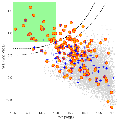
Figure 5: WISE magnitude-colour (W2, W1–W2) diagram for all 6,860 VIPERS sources (gray points). The dashed (dotted) line represents the Assef et al. (2013) selection threshold with reliability of 90% (75%). The orange circles and blue crosses represent the SED and X-ray selected AGNs, respectively. The shaded area indicates the AGN selection criteria by Stern et al. (2012)

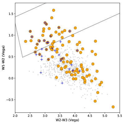
Figure 6: WISE colour-colour (W2–W3, W1–W2) diagram of the VIPERS sample with detections in all three bands (gray points) with the Mateos et al. (2012) selection wedge (dotted lines). The orange circles and blue crosses represent the SED and X-ray selected AGNs, respectively, with detections in W1, W2 and W3 bands.

First, we examined the VIPERS sample using the diagnostics of Stern et al. (2012) and Assef et al. (2013). We used the AllWISE data mentioned in Section 2.3. This sample is photometrically complete at 16.8 mag (Vega), where there is a turn-over in the number density plot of the fluxes in the W2 band. Using the Stern et al. (2012) criteria, we selected 25 AGN with magnitude brighter than W2=15.05 mag. Since this method is not reliable for fainter objects, we utilised the AGN selection criteria by Assef et al. (2013):

$${\rm{y>\alpha_{r}*exp(\beta_{r}*(x-\gamma_{r})^{2}),x>\gamma_{r}\quad}}$$ (6)

$${\rm{y>\alpha_{r},x\leq\gamma_{r},}}$$ (7)

where $x=W2$ and $y=W1-W2$ and the revised constant values of ($\alpha_{r},\beta_{r},\gamma_{r}$) given by Assef et al. (2018) are equal to ($0.650,0.153,13.86$) and ($0.486,0.092,13.07$) for the 90% and 75% reliability levels, respectively. We found 35 sources at 90% and 52 sources at 75% reliability. Figure 5 shows the WISE colour-magnitude (W1–W2 versus W2) plot for the VIPERS sample. The lines represent the wedges as defined in Assef et al. (2013) for both 90% and 75% reliability. We also over-plotted the 160 SED ($\Delta$BIC<=-2) and X-ray selected AGN samples. The shaded green area represents the Stern et al. (2012) threshold for AGN selection.

Additionally, we selected mid-IR AGNs through Mateos et al. (2012) colour selection criteria by using the colours (W2–W3) and (W1–W2). We do not apply the second diagnostic of Mateos et al. (2012) that utilizes four WISE bands as the inclusion of the W4 band with high signal-to-noise ratio reduces our sample to only 53 sources. There are 668/6,860 sources in our sample that have detections in all three bands (W1, W2 and W3) and signal-to-noise ratio greater than three. Following Mateos et al. (2012)’s criteria:

$$W1-W2<0.3150\times(W2-W3)+0.796$$ (8)

$$W1-W2>-3.172\times(W2-W3)+7.624$$ (9)

$$W1-W2>0.3150\times(W2-W3)-0.222$$ (10)

we selected 31 mid-IR AGNs. All of them are SED selected AGN by our analysis, while 29 sources are also selected by the Assef criterion with 75% reliability. In Figure 6, we plot the (W2–W3) versus (W1–W2) colours. The dotted lines define the Mateos et al. (2012) wedge. For reference, we plot the SED (orange circles) and X-ray (blue crosses) selected AGN samples. As illustrated in Figure 7 shows the Venn diagram between the different mid-IR colour selection methods. They are consistent with each other, resulting in 54 mid-IR AGNs using at least one of the aforementioned criteria.

Figure 7: Venn diagram of the AGN samples selected through the mid-IR colour selection criteria defined by Mateos et al. (2012) (red-dashed), Assef et al. (2013) (blue-solid) and Stern et al. (2012) (green-dotted).

4.4 Optical spectroscopy

We further inspected the spectra of all the SED selected AGNs to check for any AGN signature in their emission lines. In particular, we searched for the [NeV] forbidden emission line at $\lambda$=3426 Å that is often used as a diagnostic tool to distinguish between AGN and star-forming galaxies (e.g. Schmitt, 1998). Furthermore, we looked whether broad emission lines are present. Additionally, we used two optical emission line diagnostics to separate the AGN and star-forming populations: the Mass Excitation diagram (MEx, Juneau et al., 2011; Juneau et al., 2014) and the colour excitation diagram (TBT, Trouille et al., 2011), that use the ([OIII], Hb) and ([NeIII], [OII]) emission line flux ratios, respectively. For this part of our analysis, we used the latest version of the specutils packages in PYTHON.

4.4.1 [NeV] emitters and broad lines

Based on the information provided in the VIPERS spectroscopic catalogue, 27 out of the 160 SED selected AGN, present broad emission lines in their spectra. As already mentioned, the [NeV] emission line at $\lambda$=3426 Å is a good indicator of AGN activity (Schmitt, 1998; Gilli et al., 2010). Its high reliability is based on the fact that the energy needed to ionize [NeV] is 97 eV and may only come from high energy sources as opposed to, for example, stellar emission, since in the latter case the maximum emitted energy is lower than 55 eV (Haehnelt et al., 2001). The [NeV] at $\lambda$=3346 Å can also be used to identify AGN. However, it has less diagnostic power, as its intensity is significantly lower compared to [NeV] $\lambda$3426 Å (see e.g. Fig. 1 in Maddox, 2018). Many previous studies have used the [NeV] emission to select a large number of AGNs. Mignoli et al. (2013) identified 94 type 2 [NeV] emitters and compared them to X-ray selected AGN and those from line ratio diagnostics. They concluded that the [NeV] emitters can identify low-luminosity and heavily absorbed AGNs with increasing fraction to higher stellar masses. More recently, Vergani et al. (2018) studied the properties of the hosts of [NeV] AGNs, such as stellar masses, ages and colours. For the optical spectral coverage of VIPERS, the [NeV] line is accessible only for sources that lie at redshift higher than $\rm{z}>0.62$. There are 114 SED AGNs above this redshift limit. After removing objects with artefacts in their spectra and/or those with very low quality, we ended up with 42 [NeV] emitters. The vast majority of them have signal-to-noise ratio higher than five.

4.4.2 MEx and TBT diagram

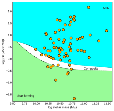
Figure 8: The Mass Excitation (MEx) diagram for the 66 SED selected AGNs that have significant both [OIII] and H$\beta$ emission lines. The dotted lines separate the star-forming galaxies from the AGNs. AGNs are found above the upper line (blue region), while under the lowest line the star-forming galaxies lie (green shaded area). In between these lines, there is a composite population that consists of both AGN and star-forming systems.

For low redshifts $\rm{z}<0.5$, the classic emission line ratio diagnostic diagram usually used is the Baldwin, Phillips, & Terlevich diagram (BPT, Baldwin et al., 1981). In our case, the standard emission lines used in the BPT diagram lie outside the wavelength coverage of the optical spectrographs. For example, for redshifts higher than $\rm{z}>0.5$ the [NII] and H$\alpha$ lines are redshifted to the observed near-IR regime. Thus, alternative indicators have been proposed in the literature, such as the rest-frame Bessel U-B galaxy colour (Yan et al., 2011, Colour Excitation diagram), H band absolute magnitude (Weiner et al., 2006), [OII]/H$\beta$ (Lamareille, 2010), Dn4000 break (Marocco et al., 2011), the stellar mass (MEx diagram) or the rest-frame colour (TBT diagram). All these replacements of the [NII]/H${\alpha}$ ratio are based on the correlation between the galaxy stellar mass and the gas phase metallicity or the rest-frame colours (depended on stellar mass; Kauffmann et al., 2003). In this work, we used the MEx and TBT diagrams.

MEx diagram avoids blending of lines in low-resolution spectra, by utilizing stellar mass and only two spectral lines, i.e., [OIII]5007 and H$\beta$. In our analysis, we used the calibrated diagram of Juneau et al. (2014) that is reliable to higher redshift (up to z$\sim$1). Using the flux ratio of [OIII] and H$\beta$ and the stellar mass of a galaxy, we utilized the mass excitation diagram to classify a source as star-forming galaxy, AGN or composite galaxy (i.e., both star-formation and AGN emission). To have both of the aforementioned lines present, we limited our sample to sources with $\rm{z}\leq 0.9$, due to the VIPERS spectral coverage. Among our 160 SED selected AGNs, 66 sources have both [OIII] and H$\beta$ lines with good quality spectra. In Figure 8, we present the MEx diagnostic plot, including the two empirically determined dividing lines of Juneau et al. (2014) that separate the pure star-forming (under), the galaxies with significant AGN emission (above) and the composite (in between) galaxies. The masses were derived from the SED fitting technique described in the previous sections. The MEx diagnostic was calibrated by using the Chabrier (2003) IMF, thus we corrected the stellar masses of our sources as we assumed initially the Salpeter (1955) IMF when we modelled the SEDs. In particular, we multiplied our stellar masses by a factor of 0.62 as found in Zahid et al. (2012). At the end, according to MEx diagnostic, 53 sources (88%) lie in the AGN area, six sources in the composite region, while seven sources in the star-forming region.

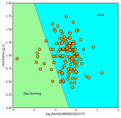
Figure 9: The TBT diagram for the 138 SED selected AGNs that have significant [NeIII] and/or [OII] emission lines. The dotted line separates the star-forming galaxies from the AGNs. The latter are found on the right part of this diagram (blue shaded region), while on the left side the star-forming galaxies exist (green shaded area).

The TBT diagram uses the rest frame colour ^0.0(g-z) as a function of the ratio of the emission lines [NeIII] and [OII]. This method relies on the assumption that AGNs are hosted by massive, fast-rotating galaxies and have high ionization lines compared to the star-forming galaxies (Zhang et al., 2019). Moreover, it is not affected by reddening, since these two lines are close to each other. An additional advantage of this method is that it can be used up to redhsift z$\sim$1.4 for optical spectra. TBT diagram is able to disentangle the star-forming galaxies from AGNs, but not the composite galaxies. However, 70% of the composite galaxies fall inside the AGN area (Pons et al., 2016). In Figure 9, the TBT diagram is shown for the 138/160 sources that have good quality spectra. The separation line (dotted) is defined as follows:

$${\rm{{}^{0.0}(g-z)=-1.2\times log([NeIII]/[OII])-0.4.}}$$ (11)

126 sources (91%) fall inside the AGN area (shaded blue), while twelve sources in the star-forming region (shaded green).

The MEx and TBT diagrams have classified seven and twelve of our SED selected AGN, as star-forming galaxies. However, 7/7 and 5/12 of these sources in the MEx and the TBT diagram, respectively, are selected as AGN through other methods (e.g. X-rays, mid-IR, [NeV] emission). Previous studies have also found a small percentage of AGN misclassified as star-forming systems, when using diagnostics based on optical spectroscopy. Juneau et al. (2011) and (Juneau et al., 2014) found 8% and 20%, respectively, of X-ray sources lying inside the star-forming regime of the MEx diagram. In our sample, there are 14 X-ray sources and 16 [NeV] emitters that fall inside the spectral coverage of MEx emission lines. 93% and 100%, respectively, are also classified as AGN based on the MEx diagram. Trouille et al. (2011) found that 3% of the X-ray sources are classified as star-forming galaxies, using the TBT diagram. In our case, the percentage of the misclassified AGNs is 5% (2/40) for the [NeV] emitters and 6.5% (2/31) for the X-ray AGNs. Given the reliability of the X-ray emission ($L_{X}>10^{42}ergs^{-1}$) and/or the significant [NeV] emission line, we assume that sources lying inside the star-forming area in both diagrams but identified as AGNs via other methods to have real AGN activity.

In total, optical spectroscopy confirms that 134/160 ($\sim$84%) SED selected AGNs present signs of AGN activity. The remaining sources mainly have poor quality spectra, thus the above diagnostics could not be applied.

4.5 Intrinsic absorption estimation

4.5.1 Mildly obscured AGNs

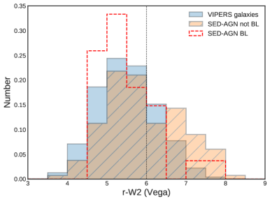
Figure 10: The normalized distribution of r–W2 colour for the SED-selected AGNs that present (red-dashed) or not (green-hatched) broad lines in their spectra. For reference, we show the histogram of the VIPERS sample classified as normal galaxies (blue). The vertical dotted line represents the threshold used in Yan et al. (2013) to select obscured AGNs.

SED fitting results revealed that 71% of the AGNs are obscured ($\psi\leq 70$ corresponding to AGNs of type 1.5 and 2), based on the estimated inclination angle (Section 4.1). However, in this section we also explore different diagnostic criteria of obscuration using optical and mid-IR colours or the X-ray to mid-IR relation.

Obscured sources are expected to be unbiased by dust in the mid-IR regime, while being absorbed in the optical bands. Yan et al. (2013) used a r–W2>6 mag cut-off along with the Stern criteria (W1–W2>0.8 and W2<15.2 mag) to select type II AGNs. LaMassa et al. (2016) used W1 instead of W2 band with a more relaxed threshold (r–W1>4 mag) in a sample of X-ray sources in Stripe 82 field and highlighted the power of this diagnostic to reveal obscured AGNs not detected through the classic W1–W2 colour criterion by Assef et al. (2013). In this work, we used the Yan et al. (2013) criteria. To be consistent with previous studies, we converted the CFHTLS r band to r_SDSS Vega system to calculate the r–W2 colour as defined by Yan et al. (2013). In Figure 10, we plot the normalized r–W2 colour distribution for the 160 high-confidence SED-selected AGNs and also the VIPERS sources classified as normal galaxies, for reference. We separate the AGN population based on whether or not broad lines are presented in their spectra. The distribution of SED-AGNs without broad lines occupies redder r–W2 colours compared to the VIPERS galaxies and broad line AGN.

To evaluate in a statistical manner if the two AGN populations come from the same distribution as the VIPERS galaxies and to assess any similarities between these samples, we performed the two-side Kolmogorov-Smirnov (KS) test. The KS test between the VIPERS galaxies and the SED-AGNs without broad lines revealed that there is a $<1.8\times 10^{-05}$ chance (D_KS=0.21) that they are drawn from the same parent population. In the case of the SED-AGNs with broad lines, we obtained a 68% probability (D_KS=0.14) for the r–W2 distributions to be representative of the same population. The SED-AGNs without broad lines have redder (r–W2=5.93) colour on average than VIPERS galaxies (r–W2=5.50) or the broad line AGNs (r–W2=5.51), while almost 40% (55/133) of them have red colours ($\rm{r-W2}\geq 6$). On the other hand, broad-line AGNs have blue colours, with the exception of only six sources being optically red. These red, type 1 AGNs have $\rm{E(B-V)}>0.05$, while most of them have $\rm{E(B-V)}=1$ that indicates a large amount of polar dust in these sources (Yang et al., 2020).

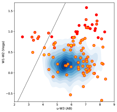
Figure 11: Optical-IR colour diagram for the 98 SED selected AGNs (filled circles). Hickox et al. (2017) selection relation is presented by the dashed line (see text for more details). Sources on the right side of this line are considered obscured. The density contours present the VIPERS sample, while the red filled circles and the crosses show the mid-IR and X-ray selected AGNs.

Hickox et al. (2017) explored the mid-IR colours and the SEDs of a large sample of type I and II quasars selected via SDSS spectroscopy. They showed that simple mid-IR colour cuts could identify the majority of luminous AGNs but may miss the most heavily obscured AGNs. On the other hand, r–W2 colour criteria might be biased against low redshift regimes (z<0.5). Thus, they defined a new optical-IR selection criterion that cleanly separates the unobscured and obscured AGNs: (u–W3[AB])>1.4$\times$(W1–W2[Vega])+3.2. This is more effective as it uses the maximum baseline between optical and IR wavelength range. However, it requires detections (or upper limits) in all four bands u, W1, W2 and W3. In Figure 11, we plot the W1–W2 versus the u–W3 colours for all the sources in the VIPERS sample requiring detections in all four bands with a minimal signal-to-noise ratio greater than two as in Hickox et al. (2017), resulting in 98 SED selected AGNs. For reference, we over-plot the AGN samples selected through mid-IR (red circles) and X-ray (crosses) selection techniques. More than 90% of the SED selected AGNs lie in the area characterized by obscuration. As expected all the sources near and on the left side of the line are unobscured broad-line AGNs.

4.5.2 Highly obscured AGNs

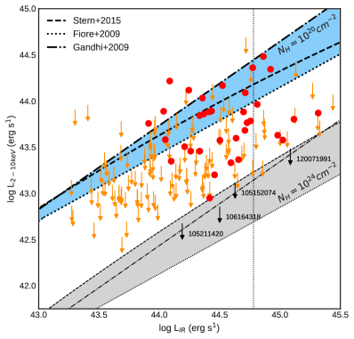
Figure 12: The X-ray luminosity in the [2-10 kev] band as a function of the IR luminosity of the SED selected AGNs with (red circles) and without (orange arrows) X-ray detections. The thick lines represent the correlation derived by (Stern, 2015), Fiore et al. (2009) and Gandhi et al. (2009) for unabsorbed AGNs. The lower thinner lines are for absorbed ($N_{H}=10^{24}$cm^-2) AGNs, assuming X-ray suppression with a factor of 20. The shaded areas correspond to the scatter of the relations derived in the aforementioned studies. The vertical line at L_IR>6$\times$10⁴⁴ erg s^-1 corresponds to our threshold for luminous sources. The thick black arrows indicate the most heavily absorbed AGNs according to this plot.

To search for sources with extreme intrinsic absorption in our sample, we used the relation of their IR and X-ray luminosity. It is well known that the mid-IR luminosity is correlated with the unabsorbed X-ray emission in the AGNs for a wide range of luminosities (Lutz et al., 2004; Gandhi et al., 2009; Mateos et al., 2015; Stern, 2015). The mid-IR emission provides a good measurement of the AGN luminosity regardless absorption. On the other hand, the X-ray emission is expected to be suppressed at some level with increasing HI column densities (Alexander et al., 2005; Alexander et al., 2008). Thus, the X-ray to mid-IR luminosity ratio constitutes another measurement of absorption. In Figure 12, we plot the X-ray luminosity in the hard band as a function of the AGN mid-IR luminosity derived by X-CIGALE. To facilitate comparison with previous studies, we transformed the luminosities from [2-8 keV] band into the [2-10 keV] band using the WebPIMMS v4.8d software, assuming a photon index of $\Gamma=1.7$ and the Galactic HI column density $N_{H}=10^{20}$cm^-2. The dashed bold line in the plot represents the relation derived from Stern (2015) from an unabsorbed AGN sample distributed over several orders of magnitude. For reference, we plot the relations given by Fiore et al. (2009) and Gandhi et al. (2009). The bottom lines indicate the corresponding relation for absorbed sources with $N_{H}=10^{24}$cm^-2. For the latter, we assumed that the X-ray emission is suppressed by a factor of 20 (Lansbury et al., 2015).

The majority of the sources lie below the Stern (2015) relation, suggesting that these are absorbed AGNs. Four sources (thick black arrows in Fig. 12) lie in the Compton-Thick (CT) regime, that suggests they may have column densities $N_{H}\geq 10^{24}$cm^-2. Figure 18 in the Appendix, presents the SEDs of these four sources. The SED fitting results show that in only one source (ID=106164318) the AGN emission is obscured in the optical wavelengths. Georgantopoulos et al. (2011), argued that even though the majority of CT sources have low L_X-L_IR ratio (at least in the local Universe), this does not necessarily imply that all sources with low L_X-L_IR ratio are CT. Furthermore, they argued that at higher redshifts, this method alone is not complete or capable to reveal real CT AGNs.

5 Discussion

Figure 13: Venn diagram of the AGN samples selected through SED decomposition (blue-solid), X-ray detection (red-dashed) and mid-IR criteria (green-dotted). These samples consists of sources that fall inside the VIPERS field, have spectroscopic redshifts from VIPERS in the range [0.5,1.2] and have optical, near-IR and mid-IR counterparts. The numbers inside parenthesis are the confirmed SED selected AGNs through optical spectroscopy.

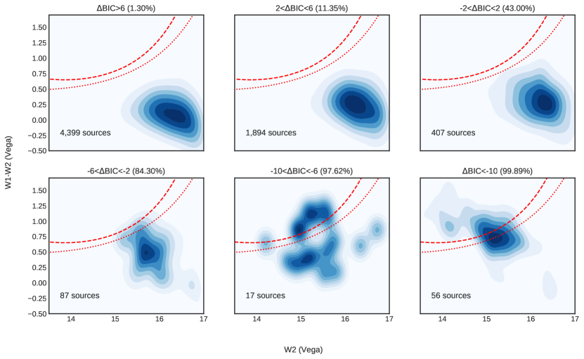
Figure 14: Density plots of the VIPERS sample in the W2, W1–W2 magnitude-colour diagram separated into bins with different $\Delta$BIC values (AGN probabilities). Above each panel, we label the range of $\Delta$BIC and in the parenthesis the average probability of the sources hosting an AGN. The dashed and dotted lines represent the AGN selection criteria defined by Assef et al. (2013) with 90% and 75% reliability, respectively.

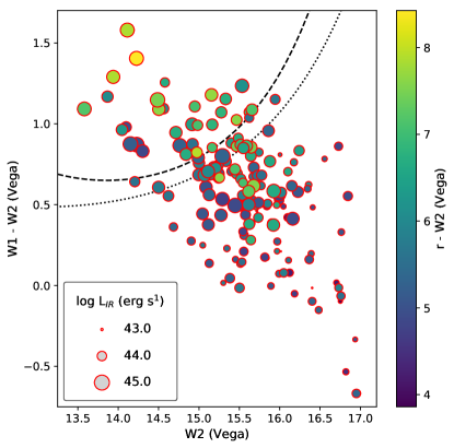
Figure 15: WISE magnitude-colour (W2, W1–W2) diagram for the 160 SED selected AGNs colour-coded based on their optical colour (r–W2). The size of the circles corresponds to the IR luminosity as indicated in the legend. The dashed (dotted) line represents the Assef et al. (2013) selection threshold with reliability of 90% (75%).

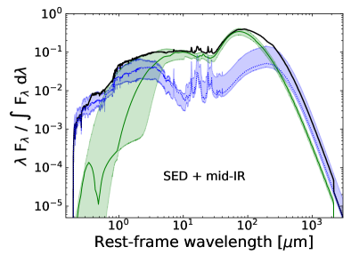
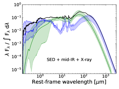
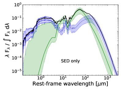
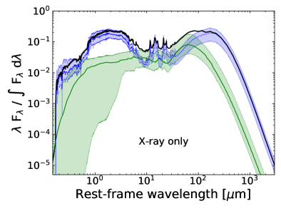
Figure 16: Stacked SEDs at rest-frame for AGN samples selected through different selection methods as indicated. The median SEDs of the host galaxy emission and the AGN components are plotted with blue dotted and green solid lines, respectively. The black thick line shows the median total flux, while the shaded areas correspond to 15^th up to 75^th percentiles at each wavelength.

The identification of AGNs in a specific wavelength regime depends strongly on the physical and observational properties of the sources, such as the luminosity, redshift, absorption and black hole mass. Thus, different selection techniques are more sensitive to different AGN populations and the overlapping among them is affected by the completeness and reliability along with the depth of each survey. To compare the various selection methods used in this work in a uniform manner, we selected the X-ray detected AGNs that have a counterpart in our initial VIPERS catalogue (with optical, near-IR and mid-IR counterparts). The Venn diagram, in Figure 13, presents the overlap of the SED (160), mid-IR (54) and X-ray (116) selected AGN samples. The numbers in the parenthesis indicate the number of confirmed AGN through optical spectroscopy ([NeV] emission, MEx and TBT diagrams). In total, 139/160 ($\sim$87%) of the SED selected AGNs revealed by our analysis, are also classified as AGN in at least one of the different AGN selection methods presented in the literature.

Specifically, all the mid-IR selected AGN (Mateos et al., 2012; Stern et al., 2012) are classified as AGN via our SED fitting technique. Regarding AGNs selected by the Assef et al. (2013) criteria (Section 4.3), 32 (44) out of 35 (52) sources with a reliability of 90% (75%), were also characterised as AGN, by our SED fitting criteria. This corresponds to a percentage of 91.5% (84.6%). The mid-IR sources not selected in our analysis have values of $\Delta$BIC lower than the threshold adopted in this work. To better understand the behaviour of $\Delta$BIC in this colour diagnostic and check if the latter sources are real AGNs, we plotted the populations defined in Table 2 in the Assef et al. (2013) diagram (Fig. 14). Starting from the upper left panel to the lower right, $\Delta$BIC is decreasing, while the probability of the sources hosting an AGN is increasing. The normal galaxy population with values $\Delta$BIC>2 (upper left and middle panels) is consistent with the mid-IR colours and all lie outside the wedges of Assef et al. (2013). In cases where it is uncertain which model describes better the observed SEDs (upper right) and the probability is equal for both galaxy and AGN templates, the majority of this population lies still below the lines. Increasing the probability of a source to host an AGN (the observed data fit better models with galaxy and AGN templates), the sources move towards the mid-IR AGN wedges defined by Assef et al. (2013) (lower panels).

Despite the relaxed threshold adopted in this work, there is a large population that would not be selected through simple colour-colour cuts. This SED selected population is twice the number of the AGN selected through the Assef et al. (2013) criteria. Figure 14 shows the robustness of the latter diagnostic criteria, but also the importance of selecting AGNs via SED decomposition techniques, as they are able to identify a much larger AGN population. SED fitting may better separate the mid-IR AGN emission from their host galaxy. In Figure 15, we plot the colour-magnitude diagram for the 160 SED selected AGNs colour-coded based on the r–W2 colour. Larger symbols correspond to higher AGN IR luminosities, derived by the SED fitting. It is evident that while the method of Assef et al. (2013) selects the brightest and optically reddest AGNs, SED decomposition allows us to identify less luminous AGNs with bluer colours.

Furthermore, among the Assef et al. (2013) selected AGNs with reliability 75% and 90%, 17 ($\sim$33%) and 14 ($\sim$40%) sources have X-ray emission, respectively. Mendez et al. (2013) showed that the percentage of mid-IR selected AGNs that have X-ray detections depends strongly on the depths of the surveys and ranges between 45% to 90%. When the depth of the IR surveys increases, this fraction decreases. On the other hand, increasing the X-ray depth increases the fraction of mid-IR AGNs that are X-ray detected. For example, Pouliasis et al. (2019) found that $\sim$70% of mid-IR AGNs have X-ray detections in the $\sim$7 Ms Chandra Deep Field South (CDFS) image. Our results agree well with those of Mendez et al. (2013) for shallow depth X-ray surveys (in this work the average is $\sim$20 ks) and low sensitivity limits in the IR bands. The majority of the X-ray sources lie outside the mid-IR wedges (Fig. 5). This could be due to the fact that these sources may be less luminous in mid-IR or that the relative emission from the host galaxy overpowers that from the AGN. Sources inside the Assef et al. (2013) wedge with no X-ray counterparts are expected to be luminous absorbed AGNs. Out of these, 12/37 ($\sim$33%) have [NeV] emission in their optical spectra while the vast majority have red colours.

Finally, $\sim$21% of the SED selected AGNs have X-ray emission. On the other hand, we found that 30% of the X-ray population is selected as AGN via SED decomposition with high significance. As shown in Table 2, the majority of the X-ray sources have low AGN probabilities, based on our Bayesian analysis. One possible explanation is that these sources do not have a large enough amount of dust around their black hole to overpower the host galaxy luminosity. Indeed, the average IR AGN luminosity for X-ray sources that are not selected through SED decomposition is almost 0.5 dex lower compared to SED selected AGNs. The SED decomposition is biased towards those objects which are bright in the infrared compared to their hosts, and so this would naturally directly lead to this difference. In order to visualize these results, we plot in Figure 16 the stacked SEDs for AGN samples identified via different combinations of AGN selections methods. AGNs selected through the SED fitting technique, mid-IR colours and are detected in X-rays (upper right panel) are in general AGN-dominated systems. Furthermore, the median AGN emission extends to the optical wavelengths which indicates that these are less obscured sources. In the case of AGN that are SED and mid-IR selected (upper left panel) the AGN component is dominant but the AGNs are more obscured. Similarly, the SED-only selected sample (bottom left panel) consists of obscured AGNs, though with less dominant AGN component. In contrast, the X-ray only selected AGNs (lower right panel) comprise systems that the host galaxy component dominates the SED. The scatter in the AGN emission in those stacked SEDs, especially in the optical regime of the spectrum, is mostly due to the different types of AGN (obscured, unobscured, intermediate type).

Taking into account only sources with high mid-IR luminosity, 7 out of 21 sources ($\sim$34%) have an X-ray counterpart. The luminosity cut at L_IR>6$\times$10⁴⁴ erg s^-1 (vertical line in Fig. 12) was defined in Del Moro et al. (2016) and corresponds to the X-ray quasar regime according to the L_X-L_IR relation. Del Moro et al. (2016) found that 70% of mid-IR luminous AGNs in the redshift range 1<z<3 is detected in the X-rays. This discrepancy comes partially from the different redshift regime and mostly from the depth of their X-ray observations (2 and 4 Ms) Chandra X-ray observations compared to the XMM-Newton observations used in this study with much lower exposure times ($\sim$20 ks). In Mountrichas et al. (2017), the obscured fraction among a sample of type I AGNs (average redshift equal to 2.3) with luminosities higher than L_IR>1.6$\times$10⁴⁶ erg s^-1 was found $\sim$10%. This indicates a higher number of absorbed sources at higher redshifts and type I AGNs. Finally, 10/21 of these sources are also [NeV] emitters, while the majority of them are classified as optically red (r–W2$\geq$6). Example SEDs of the luminous mid-IR AGNs with and without X-ray detections are shown in Figure 17 in the Appendix B.

6 Summary and Conclusions

AGN selection based on X-ray emission is by far the most reliable and effective tool to select a large number of AGNs. However, it is biased against the most absorbed ones. SED fitting techniques in the mid-IR regime are able to disentangle the IR emission coming from the torus, which is heated by the central engine from the host galaxy, and identify these populations that X-ray selection misses. In this work, we built and modelled the SEDs of 6,860 sources in the CFHTLS W1 field, using the X-CIGALE software. All sources in this sample have spectroscopic redshifts from the VIPERS survey and have been observed in optical (CFHTLS), near-IR (VHS) and mid-IR (WISE) photometric bands. We fitted these SEDs with galaxy only templates and in a second run we combined both galaxy and AGN templates. Using a Bayesian approach, we compared these two fits and selected the objects for which the addition of an AGN component provides a higher statistical confidence level.

We ended up with 160 sources with high AGN probability. Analysis of their optical spectra revealed 27 broad line AGNs, with 42/114 (37%) inside the spectral coverage having [NeV] emission. Using the MEx and TBT diagrams, 90% of our SED selected AGNs, with the corresponding emission lines detected, fall inside the AGN or composite areas in these diagrams. In total, 134/160 (84%) of our SED selected sources are confirmed AGNs, by these robust diagnostic tools. Our main results can be summarized as follows:

• To compare our SED decomposition technique with mid-IR selection methods that identify AGN, we applied the selection criteria of Assef et al. (2013), Stern et al. (2012) and Mateos et al. (2012). Our analysis revealed that the SED method recovers the mid-IR AGN population with high completeness (92%). However, we found in addition a significant number of AGNs, twice as high as with mid-IR colour techniques. This population that simple mid-IR colours fail to uncover consists of lower luminosity AGNs with systems that are dominated by the host galaxy emission.

• Among the X-ray selected AGNs, 34/116 (30%) sources are selected through our SED analysis method. The remaining X-ray population not selected through SED fitting has host-galaxy dominated systems. On the other hand, 34/160 (21%) of the SED selected AGNs have X-ray emission. In addition to this, the SED fitting results suggest that the vast majority ($\sim$70%) of the AGNs have inclination angles of view $\psi\leq 50$ indicating some level of obscuration (type 1.5 and 2). We verify these results using the optical and mid-IR colour selection criteria defined by Yan et al. (2013) and Hickox et al. (2017) and utilizing the L_X-L_IR diagram. Interestingly, only 35% of the most luminous mid-IR selected AGNs have X-ray counterparts, suggesting strong absorption].

We conclude that the different methods (SED decomposition, mid-IR colours, X-ray emission) used to identify AGNs are complementary to each other and equally important to constrain the full picture of the AGN demographics. In particular, SED fitting is able to identify a large number of obscured AGNs that the X-ray surveys miss and the simple mid-IR colour cuts do not select. These are critical for studying the AGN population with high obscuration in host-galaxy dominated systems and it might be the key between the connection of normal galaxies and AGNs.

Appendix A Bayesian factor

To compare models in Bayesian statistics, one needs to calculate the Bayes factor, BF, that is the ratio of the posteriori to a priori complementary probabilities (or the so-called evidence ratio). Let’s assume that two models (m₁, m₂) have to be compared to a specific data set y and p₁, p₂ their parameters, respectively. Applying the Bayes theorem, the posteriori probabilities for the two models are:

$$\centering f(\textbf{m\textsubscript{1}}|\textbf{y})=\frac{f(\textbf{m\textsubscript{1}})f(\textbf{y}|\textbf{m\textsubscript{1}})}{\sum\limits_{i=1}^{2}f(\textbf{m\textsubscript{i}})f(\textbf{y}|\textbf{m\textsubscript{i}})}\quad\text{and}\quad f(\textbf{m\textsubscript{2}}|\textbf{y})=1-f(\textbf{m\textsubscript{1}}|\textbf{y}).\@add@centering$$ (12)

Then, we calculate the ratio of the posteriori complementary probabilities of the two models (posterior odds, $\textbf{PO}=\frac{f(\textbf{m\textsubscript{1}}|\textbf{y})}{f(\textbf{m\textsubscript{2}}|\textbf{y})}$) and also the Bayes factor of model m₁ against model m₂:

$$\centering\begin{multlined}\textbf{BF}=\frac{f(\textbf{m\textsubscript{1}}|\textbf{y})/f(\textbf{m\textsubscript{2}}|\textbf{y})}{f(\textbf{m\textsubscript{1}})/f(\textbf{m\textsubscript{2}})}\\ =\frac{[\frac{f(\textbf{m\textsubscript{1}})f(\textbf{y}|\textbf{m\textsubscript{1}})}{\sum\limits_{i=1}^{2}f(\textbf{m\textsubscript{i}})f(\textbf{y}|\textbf{m\textsubscript{i}})}]/[\frac{f(\textbf{m\textsubscript{2}})f(\textbf{y}|\textbf{m\textsubscript{2}})}{\sum\limits_{i=1}^{2}f(\textbf{m\textsubscript{i}})f(\textbf{y}|\textbf{m\textsubscript{i}})}]}{f(\textbf{m\textsubscript{1}})/f(\textbf{m\textsubscript{2}})}=\frac{f(\textbf{y}|\textbf{m\textsubscript{1}})}{f(\textbf{y}|\textbf{m\textsubscript{2}})},\end{multlined}\textbf{BF}=\frac{f(\textbf{m\textsubscript{1}}|\textbf{y})/f(\textbf{m\textsubscript{2}}|\textbf{y})}{f(\textbf{m\textsubscript{1}})/f(\textbf{m\textsubscript{2}})}\\ =\frac{[\frac{f(\textbf{m\textsubscript{1}})f(\textbf{y}|\textbf{m\textsubscript{1}})}{\sum\limits_{i=1}^{2}f(\textbf{m\textsubscript{i}})f(\textbf{y}|\textbf{m\textsubscript{i}})}]/[\frac{f(\textbf{m\textsubscript{2}})f(\textbf{y}|\textbf{m\textsubscript{2}})}{\sum\limits_{i=1}^{2}f(\textbf{m\textsubscript{i}})f(\textbf{y}|\textbf{m\textsubscript{i}})}]}{f(\textbf{m\textsubscript{1}})/f(\textbf{m\textsubscript{2}})}=\frac{f(\textbf{y}|\textbf{m\textsubscript{1}})}{f(\textbf{y}|\textbf{m\textsubscript{2}})},\@add@centering$$ (13)

where $f(\textbf{y}|\textbf{m\textsubscript{i}})$ is the marginal likelihood (or the so-called evidence) of the i model and is calculated by integrating with respect to parameters of each model:

$$\centering f(\textbf{y}|\textbf{m\textsubscript{i}})=\int f(\textbf{y}|\textbf{k\textsubscript{i}},\textbf{m\textsubscript{i}})f\textsubscript{i}(\textbf{p\textsubscript{i}})d\textbf{p\textsubscript{i}},\quad i=1,2.\@add@centering$$ (14)

The value of the Bayes factor determines the rejection or not of the initial assumption with high values (>1) indicating evidence in favor of that model. In practice, the Bayes factor is a measure of the weight of the information that is included in the data in a favor of one model against an other. It can be used as a relative measurement for the comparison of the two models. Kass & Raftery (1995) gave the possible explanation of the Bayes factor for the comparison between two models that are shown in Table 2.

Appendix B SEDs and properties of the SED selected AGNs

Figure 17 presents some example SEDs of the 21 luminous AGNs with L_IR>6$\times$10⁴⁴ erg s^-1 with and without X-ray detections, while Figure 18 shows the SEDs for four Compton Thick candidates according to the L_X-L_IR diagram. In Table 4, we list the observational and physical properties of all the 160 SED selected AGNs.

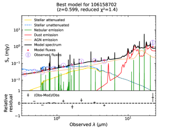
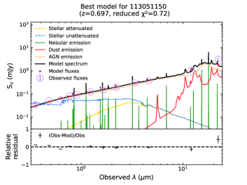
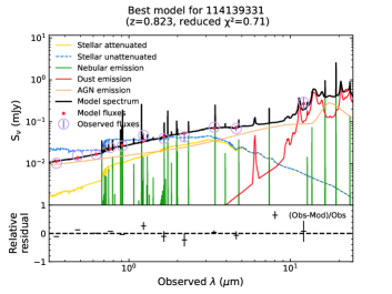
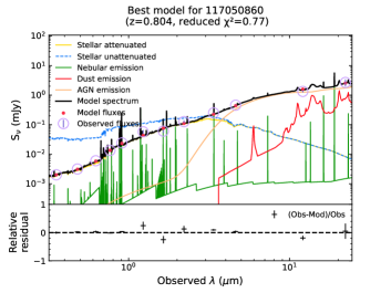
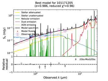
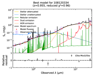
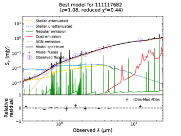
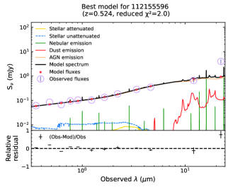
Figure 17: Example SEDs of eight luminous AGNs (L_IR>6$\times$10⁴⁴ erg s^-1) with (upper four) and without (lower four) X-ray detections. The dust emission is plotted in red, the AGN component in green, and the attenuated (unattenuated) stellar component is shown with the yellow (blue) solid (dashed) line, while the orange lines shows the nebular emission. The total flux is represented with black colour. Below each SED, we plot the relative residual fluxes versus wavelength.

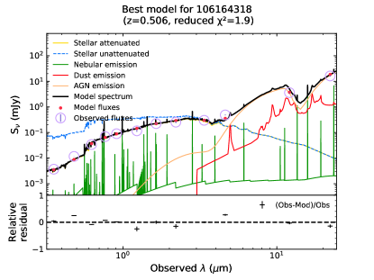
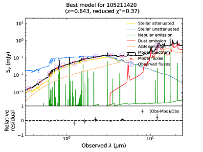
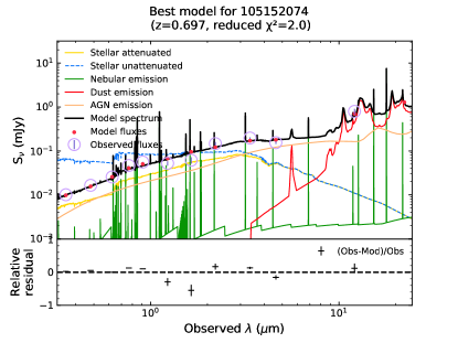
Figure 18: SEDs of the four AGNs with extreme obscuration according to the L_X–L_IR relation. The dust emission is plotted in red, the AGN component in green, and the attenuated (unattenuated) stellar component is shown with the yellow (blue) solid (dashed) line, while the orange lines shows the nebular emission. The total flux is represented with black colour. Below each SED, we plot the relative residual fluxes versus wavelength.

Table 3: Catalogue of the 160 SED selected AGNs.

VIPERS	RA	DEC	z	LIR	LX	mid-IR	Broad	[NeV]	MEx	TBT	SED	r–W2
ID	(J2000)	(J2000)		(erg s-1)	(erg s-1)	AGN	lines	emission	AGN	AGN	AGN type	(Vega)
(1)	(2)	(3)	(4)	(5)	(6)	(7)	(8)	(9)	(10)	(11)	(12)	(13)
101128062	30.44515	-5.94690	0.652	43.93	<43.68	0	0	0	0	1	2.0	4.76
101143290	30.65517	-5.87594	0.736	44.07	<43.68	0	0	0	0	1	2.0	4.94
101145879	31.06676	-5.85939	0.529	43.51	<42.89	0	0	0	0	1	2.0	4.93
101166083	30.97806	-5.76278	0.516	43.46	<42.70	0	0	0	0	0	2.0	4.63
101167170	30.61551	-5.75817	1.029	45.06	<43.68	0	0	0	0	0	2.0	6.64
101171205	30.42398	-5.74079	0.986	44.86	<43.92	0	1	1	0	1	1.0	4.92
101175047	30.91564	-5.72366	0.549	43.77	<43.28	0	0	0	0	1	1.5	5.99
101183266	31.14391	-5.68359	0.690	44.26	<43.68	0	0	0	0	1	1.5	5.75
101184375	30.53652	-5.68232	0.655	43.93	<43.65	0	0	0	0	0	2.0	4.85
101199625	30.43171	-5.60912	0.530	43.30	<43.92	0	0	0	1	1	2.0	5.39
102121299	32.02825	-5.96117	0.538	44.33	43.84	1	0	0	1	1	2.0	6.02
102129812	31.40485	-5.92148	0.817	43.95	<43.42	0	0	0	0	0	1.5	6.63
102133752	31.33519	-5.90048	0.537	44.04	43.89	0	0	0	1	0	1.0	5.36
102138525	31.56050	-5.87794	0.797	44.57	<43.60	0	0	0	1	1	1.5	6.22
102178761	31.22399	-5.67968	0.689	43.68	<43.54	0	0	1	0	1	2.0	4.70
102183859	31.62379	-5.65619	0.599	43.69	<43.09	0	0	0	0	0	2.0	5.09
103134908	32.21963	-5.97658	0.644	44.37	<43.13	0	0	0	1	1	1.5	4.84
103143919	32.29891	-5.93776	0.773	44.76	43.78	1	1	1	0	1	1.0	7.63
103151883	32.35777	-5.90568	0.636	45.12	43.80	1	1	1	0	0	1.0	5.29
103180263	32.25861	-5.78499	0.644	44.71	43.68	0	1	0	0	1	1.0	5.14
103180825	32.77869	-5.78191	0.748	44.73	43.77	0	1	0	0	1	1.5	5.19
103197293	32.67400	-5.71261	0.664	43.52	<43.30	0	0	1	0	1	2.0	5.76
104170739	33.70780	-5.90915	0.715	43.80	<43.26	0	0	0	1	1	2.0	4.22
104236309	33.97194	-5.65539	0.546	43.85	<43.03	0	0	0	0	0	1.0	6.34
105139296	34.09171	-5.95674	1.048	44.14	<43.88	0	0	1	0	1	2.0	6.88
105145409	34.09651	-5.93140	1.095	44.51	<43.71	0	0	1	0	1	2.0	6.54
105152074	34.22651	-5.90089	0.697	44.63	<43.13	0	0	1	1	1	1.0	5.11
105189949	34.16295	-5.72786	0.643	43.55	<43.16	0	0	0	1	1	2.0	6.01
105201540	34.64631	-5.67718	0.851	44.58	<43.63	0	0	0	0	1	1.0	5.37
105211420	34.71244	-5.62929	0.643	44.19	<42.69	0	0	0	1	1	1.0	5.88
105216790	34.47889	-5.60829	0.843	44.39	<43.43	1	0	0	1	0	1.5	7.61
106158702	35.13075	-5.87612	0.599	45.02	43.58	0	1	0	0	1	1.5	4.72
106164318	35.79339	-5.85072	0.506	44.50	<42.87	1	0	0	1	1	2.0	6.06
106204876	35.60449	-5.66945	1.078	44.44	<44.20	1	0	1	0	0	2.0	6.94
106208862	35.82120	-5.65156	0.802	43.88	<43.50	0	0	0	0	1	2.0	5.95
107161301	36.85607	-5.65162	1.077	44.57	<43.72	1	0	1	0	1	2.0	7.15
108114624	37.12663	-5.97348	0.553	43.55	<43.46	0	0	0	1	1	2.0	5.36
108120334	37.46318	-5.94224	0.955	45.12	<43.94	1	0	1	0	1	2.0	7.86
108137534	37.02236	-5.85604	0.778	44.70	43.88	1	1	1	0	1	2.0	5.40
108163578	37.59208	-5.70686	0.716	44.68	<43.53	1	0	0	1	1	1.0	5.67
108167635	37.26583	-5.68088	1.043	44.87	<43.77	1	1	1	0	1	1.0	6.05
108168148	37.07837	-5.68167	0.626	43.93	<43.56	0	0	0	1	1	1.5	6.10
109130669	38.48938	-5.91916	0.554	43.99	<42.89	0	0	0	1	1	2.0	4.74
109161838	38.20769	-5.76429	1.102	44.28	<43.76	0	0	1	0	1	2.0	6.44
109164682	38.43727	-5.74709	0.825	44.42	<43.14	0	0	0	0	0	1.0	6.70
109179237	38.46824	-5.67911	0.593	43.44	<43.06	0	0	0	1	1	2.0	3.86
110043474	31.13770	-5.43120	0.666	44.55	<43.55	1	0	1	1	1	1.0	5.63
110054196	31.15407	-5.37707	0.596	44.77	<43.38	0	1	0	0	1	1.0	5.02
110066563	30.80605	-5.31692	0.696	43.82	<43.04	0	0	0	0	1	2.0	5.78
110072899	30.28438	-5.28715	0.776	44.51	<43.95	1	0	1	1	1	1.5	6.81
110078074	30.76310	-5.26278	0.512	43.66	<43.09	0	0	0	0	1	2.0	5.64
110100629	30.69404	-5.15765	0.859	44.09	44.22	0	1	0	0	1	1.0	6.01
110133664	30.77885	-5.00982	0.507	43.67	<43.11	0	0	0	1	1	2.0	6.06
110180344	30.94828	-4.79023	0.617	44.02	<43.31	0	0	0	1	1	1.5	5.92
110202029	30.44836	-4.68994	0.558	43.96	<43.55	0	0	0	0	1	2.0	5.46
110204490	30.46040	-4.67859	0.764	44.08	<43.81	1	0	1	1	1	2.0	5.60
111063425	31.62215	-5.31458	0.613	43.91	<42.98	0	0	0	0	1	1.5	5.69
111076897	31.61439	-5.24968	0.963	44.37	43.86	0	1	1	1	1	1.0	5.59
111108509	31.47468	-5.10136	1.135	44.53	<44.06	0	0	0	0	0	2.0	6.62
111117682	31.51571	-5.05702	1.084	45.27	<44.21	1	0	1	0	1	1.5	7.51
111120886	31.32135	-5.04079	0.516	43.90	<43.12	0	0	0	0	1	2.0	5.26
111153701	31.84755	-4.88503	0.704	44.30	<43.37	1	0	1	1	1	1.5	6.38
111157163	31.98383	-4.86751	0.557	43.73	<42.71	0	0	0	1	1	2.0	5.36
111161925	31.35488	-4.84550	1.093	44.70	<43.57	0	0	1	0	0	2.0	7.30
111192162	31.88525	-4.70298	0.500	44.42	42.92	0	0	0	0	0	1.5	5.33
112032836	32.35279	-5.47099	0.649	44.21	<43.52	0	0	0	0	1	1.0	4.95
112071341	32.94422	-5.28638	0.789	44.49	<43.71	1	0	1	1	1	1.5	6.83
112089875	32.39088	-5.19864	0.620	43.74	<43.21	0	0	0	0	1	2.0	5.27
112100049	33.02364	-5.15279	1.035	44.87	<43.83	0	0	0	0	0	2.0	7.58
112105956	32.70154	-5.12298	0.565	43.95	<43.33	0	0	0	0	0	1.0	4.80
112130497	32.44284	-5.01467	0.983	44.58	<44.03	0	0	1	0	1	2.0	7.47
112141684	33.06693	-4.96233	0.983	44.77	44.36	1	0	0	0	0	2.0	7.69
112155596	32.76740	-4.89028	0.524	45.33	<43.80	1	1	0	0	1	1.5	4.94
112163489	33.00277	-4.85407	0.754	44.40	<43.35	1	0	0	1	1	1.5	7.42
112167778	32.26360	-4.83555	0.843	44.86	<43.37	1	0	0	1	1	1.5	6.47
112169655	32.31060	-4.82707	0.655	44.23	<43.18	1	0	0	0	1	1.0	7.05
112173291	33.05381	-4.81045	0.507	43.44	<43.18	0	0	0	1	1	2.0	5.41
112196243	32.45579	-4.70356	0.701	43.85	<43.25	0	0	0	0	1	2.0	5.35
113037156	33.96294	-5.45440	0.641	44.36	<43.22	0	0	0	1	0	1.0	6.48
113044521	33.32085	-5.42048	1.014	44.86	44.48	0	1	1	0	1	1.0	6.09

• Note. – (1): Identifier. (2): Right ascension. (3): Declination. (4): Redshift. (5): Infrared AGN luminosity. (6): X-ray [2-10 keV] luminosity. The ’<’ symbol represent the upper limit. (7): "1" ("0") if AGN is (is not) selected through mid-IR colours. (8): "1" ("0") for existence (absence) of broad lines. (9), (10), (11): "1" ("0") if AGN is (is not) selected via [NeV] emission, MEx and TBT diagrams, respectively. (12): AGN type derived from the SED fitting results ($\psi$ value). (13): r–W2 colour (Yan et al., 2013).

Table 4: continued

VIPERS	RA	DEC	z	LIR	LX	mid-IR	Broad	[NeV]	MEx	TBT	SED	r–W2
ID	(J2000)	(J2000)		(erg s-1)	(erg s-1)	AGN	lines	emission	AGN	AGN	AGN type	(Vega)
(1)	(2)	(3)	(4)	(5)	(6)	(7)	(8)	(9)	(10)	(11)	(12)	(13)
113051150	33.34912	-5.38764	0.697	45.32	43.87	1	1	0	0	1	1.5	5.23
113064992	33.13933	-5.32305	0.540	43.27	<43.16	0	0	0	1	1	2.0	5.05
113092199	33.45236	-5.19618	0.585	43.95	<43.03	0	0	0	1	1	2.0	5.42
113110546	33.99779	-5.11639	0.500	44.10	43.35	1	0	0	1	1	2.0	6.66
113169191	33.07584	-4.85186	0.742	43.53	<43.16	0	0	0	0	0	2.0	4.73
113180911	33.82514	-4.80045	0.624	43.68	<43.06	0	0	0	0	0	2.0	5.18
113206860	33.08376	-4.67540	0.807	43.97	<43.85	0	0	0	0	1	2.0	5.37
114073711	34.67060	-5.31094	0.659	44.23	<43.29	0	0	0	1	1	2.0	6.44
114082043	34.38863	-5.26415	0.599	44.36	44.03	0	0	0	0	0	1.0	5.66
114108550	34.74651	-5.16858	0.753	44.65	<43.24	1	0	0	1	1	1.0	6.70
114131874	34.58537	-5.07403	0.649	44.52	44.17	1	1	0	0	1	1.5	6.32
114139331	34.32735	-5.04438	0.823	44.98	43.63	0	1	1	0	1	1.0	4.68
114161732	34.28235	-4.95660	1.092	44.61	<43.95	0	0	0	0	1	1.0	6.98
115027291	35.78914	-5.49197	0.626	44.26	43.46	1	0	0	1	1	2.0	5.59
115115472	35.66146	-5.06443	0.907	44.05	43.58	0	1	1	0	1	1.0	7.31
115122976	35.65010	-5.02796	0.845	44.24	44.12	0	0	1	1	1	2.0	7.63
115135448	35.82728	-4.97046	0.828	44.41	43.88	1	0	0	1	1	1.0	7.91
116014737	36.78589	-5.55085	0.553	44.16	<43.32	0	0	0	1	1	1.0	6.18
116032161	36.57659	-5.45495	0.770	43.68	<43.80	0	0	1	1	1	2.0	5.65
116042241	36.60305	-5.40163	1.000	44.76	<44.39	0	0	1	0	1	2.0	6.63
116046207	36.75194	-5.38182	0.870	45.31	<43.87	0	1	1	0	1	1.5	4.88
116085907	36.02205	-5.18092	0.649	43.69	<42.54	0	0	0	0	1	1.0	6.67
116099542	36.73734	-5.11584	0.704	43.58	<43.27	0	0	1	1	1	2.0	5.74
116150199	36.37517	-4.87492	0.629	43.72	<43.03	0	0	0	0	1	2.0	5.43
116167222	36.39511	-4.79289	0.854	44.17	<43.40	1	0	1	1	1	2.0	6.68
116192311	35.95629	-4.66974	0.622	44.21	43.51	0	0	0	1	1	2.0	5.84
117010534	37.79089	-5.57627	0.986	45.13	<44.44	1	0	0	0	1	1.5	8.43
117027325	37.62852	-5.49188	0.784	43.88	<43.44	0	0	0	0	1	2.0	5.54
117037264	37.08046	-5.44453	0.786	44.44	<43.46	1	0	0	1	1	2.0	7.08
117050860	36.96234	-5.37541	0.804	44.92	44.34	1	0	1	1	1	2.0	7.86
117062279	37.26845	-5.31627	0.779	43.96	<43.54	0	0	0	0	1	2.0	5.85
117066130	37.84448	-5.29393	0.586	43.92	<43.37	0	0	0	1	1	2.0	5.09
117110515	37.15691	-5.09081	0.698	43.49	<43.03	0	0	0	0	1	2.0	5.04
117135140	37.13011	-4.97454	0.933	44.05	<43.71	0	0	0	0	0	2.0	4.99
117173795	37.68207	-4.76728	0.630	43.56	<43.37	0	0	0	0	1	2.0	4.17
117177187	37.35116	-4.75558	0.892	44.30	<43.49	1	0	0	0	1	2.0	7.08
117178247	37.36978	-4.74554	0.610	44.66	43.37	0	0	0	1	1	1.0	4.87
117186794	37.30807	-4.70517	0.662	43.91	43.76	0	1	0	0	1	1.5	5.81
118042646	38.32293	-5.41092	0.708	44.63	<43.34	0	1	1	0	1	1.0	5.79
118086325	38.44772	-5.18750	0.638	44.22	<44.14	1	0	0	1	1	1.0	5.72
118086892	38.49890	-5.18475	0.516	43.41	<43.97	0	0	0	0	0	2.0	5.61
118086923	38.28170	-5.18458	0.731	44.12	<43.10	0	0	1	1	1	1.0	6.38
118087346	38.60147	-5.18252	0.803	44.55	<43.83	1	0	0	0	0	1.5	6.74
118128010	38.48948	-4.98375	0.646	43.74	<43.46	0	0	0	1	1	2.0	5.38
118161115	38.01033	-4.80912	0.543	43.28	<42.83	0	0	0	1	1	2.0	5.13
118187397	38.10186	-4.67423	0.763	44.22	<43.28	1	0	0	1	1	2.0	7.06
119009735	30.37515	-4.64988	0.894	44.72	<44.70	1	0	1	0	1	2.0	6.72
119034376	30.75731	-4.53195	0.939	44.08	<43.56	0	0	0	0	1	2.0	6.54
119061358	30.48839	-4.39574	0.549	43.96	<43.81	1	0	0	0	0	1.5	7.23
119088613	31.14702	-4.26421	0.578	43.83	<42.87	0	0	0	0	1	2.0	4.61
119091830	30.98208	-4.25297	0.735	44.14	<43.34	0	0	0	0	0	2.0	5.74
119095831	30.75257	-4.22947	0.525	43.64	<42.92	0	0	0	0	0	2.0	5.17
120040724	31.90079	-4.52882	0.971	44.27	<43.85	0	1	0	0	1	1.0	5.52
120071991	31.39916	-4.39738	0.741	45.08	<43.50	1	0	0	1	1	1.0	7.19
120103089	31.84380	-4.27291	0.707	44.46	43.20	0	1	0	0	1	1.5	5.10
120114522	32.09921	-4.22791	0.745	44.39	<43.36	1	0	1	1	1	1.0	6.69
121034054	32.41920	-4.54024	0.591	43.62	<43.30	0	0	0	0	0	2.0	5.44
121043880	32.91610	-4.48952	0.851	44.38	<43.34	0	0	0	0	1	1.5	5.95
121046919	32.42821	-4.47505	0.533	44.81	43.96	1	1	0	0	1	1.5	4.82
121062481	32.42717	-4.40335	0.842	44.42	<43.51	0	0	0	0	0	1.5	7.13
121099761	32.53067	-4.24116	0.822	43.93	<43.40	0	0	1	1	1	2.0	5.56
121102071	32.87646	-4.23080	0.609	44.33	43.46	1	1	0	0	1	1.0	4.95
122022800	33.37111	-4.57965	0.674	44.64	43.60	0	1	1	0	1	1.0	5.43
122042685	33.50952	-4.48348	0.514	43.82	<43.06	0	0	0	1	1	1.0	4.12
122043807	33.72362	-4.47911	0.722	44.80	<43.67	0	0	0	0	1	2.0	5.86
122052858	33.11464	-4.43304	1.149	45.44	<44.08	1	1	0	0	0	1.0	5.31
122100077	33.17477	-4.21485	0.669	44.50	43.57	1	0	1	1	1	1.0	5.87
123021037	34.20095	-4.59600	0.502	43.27	<42.88	0	0	0	1	1	2.0	4.46
123057675	34.49237	-4.42283	0.646	44.43	43.89	0	0	1	1	1	1.0	5.08
123098574	34.78088	-4.24129	0.660	43.97	<43.00	0	0	0	0	1	2.0	5.14
124035576	35.84055	-4.52366	0.619	44.09	<43.16	0	0	0	0	0	1.5	4.82
124072245	35.24707	-4.36030	0.812	44.36	<43.20	0	0	0	0	0	1.0	5.36
124075097	35.57515	-4.34718	0.837	44.11	<43.24	0	0	0	0	1	1.0	7.06
124109737	35.53904	-4.19366	0.616	44.14	<43.13	0	0	0	0	1	2.0	5.32
125022958	36.15360	-4.58911	0.639	43.63	<43.04	0	0	0	0	0	2.0	4.44
125026840	36.42350	-4.57150	0.611	44.26	<43.04	0	1	0	0	1	1.5	5.78
127028630	38.34431	-4.55794	0.578	44.59	43.33	0	0	0	1	1	1.0	5.09
127061363	38.40941	-4.39736	0.753	44.71	44.09	1	0	0	1	1	1.0	5.76
127103639	38.46575	-4.21191	1.150	45.00	<43.70	1	0	1	0	0	1.5	6.16
127111323	38.32294	-4.17705	0.658	43.61	<43.11	0	0	0	0	1	2.0	5.63

• Note. – (1): Identifier. (2): Right ascension. (3): Declination. (4): Redshift. (5): Infrared AGN luminosity. (6): X-ray [2-10 keV] luminosity. The ’<’ symbol represent the upper limit. (7): "1" ("0") if AGN is (is not) selected through mid-IR colours. (8): "1" ("0") for existence (absence) of broad lines. (9), (10), (11): "1" ("0") if AGN is (is not) selected via [NeV] emission, MEx and TBT diagrams, respectively. (12): AGN type derived from the SED fitting results ($\psi$ value). (13): r–W2 colour (Yan et al., 2013).

Appendix C Dependence of the method’s reliability on the available photometry

In our analysis, we constructed SEDs using optical, near-IR and mid-IR photometry. In this section, we examine the effect of adding ancillary data on the reliability of our method. In particular, we test if the omission of (i) near-IR photometry, (ii) the longest mid-IR photometric bands and (iii) the addition of far-IR data, affects the AGN selection method. Toward this end, we followed the procedure described in Section 3 to calculate the $\Delta$BIC values for all samples with different number of photometric bands. Then, we compared these values assuming that real AGNs are the SED-AGNs derived from the sample with the highest number of bands used.

Our analysis revealed, that the absence of near-IR data results in a high number of false-positive AGN identifications. For relaxed thresholds ($\Delta$BIC<-2), even though the completeness is high (62%), the false-positive rate reaches up to 65% overestimating the number of the selected AGNs. This is probably due to the fact that in these bands the AGN and galaxy SEDs are almost equal in fluxes. Thus, we chose to include near-IR bands in our analysis to better constraint the SED fitting and increase the reliability of our method. Furthermore, we tested if the absence of both the W3 and W4 bands affects the reliability of the AGN selection method. Comparing the SED selected samples, we concluded that the absence of W3 and W4 bands resulted in 16% of false-positive AGN candidates. W3 and W4 photometric bands are available for 86% of the galaxies in the VIPERS sample. Thus, we expect $\sim 2\%$ of our SED selected AGN to be misclassified.

We also examined whether the addition of far-IR data affects the AGN selection method. For that purpose, we used the Herschel Multi-tiered Extragalactic Survey (HerMES) data (Oliver et al., 2012) that overlap with the VIPERS field. HerMES used PACS (Poglitsch et al., 2010) and SPIRE (Griffin et al., 2010) photometric data from the ESA Herschel Space Observatory (Pilbratt et al., 2010). We cross-matched the VIPERS sample with the far-IR sources as described in Section 2.5. For the 174 sources with Herschel data, we run the X-CIGALE code with and without AGN templates. We, then, compared the SED selected AGNs and we found no statistical differences between the results. Thus, in our analysis, we do not require far-IR photometry. This does not affect the reliability of our method, while it allows us to apply the methodology in a significantly larger galaxy sample.

References

- Akaike (1974) Akaike H., 1974, IEEE Transactions on Automatic Control, 19, 716
- Akylas et al. (2012) Akylas A., Georgakakis A., Georgantopoulos I., Brightman M., Nandra K., 2012, A&A, 546, A98
- Alexander et al. (2003) Alexander D. M., et al., 2003, The Astronomical Journal, 125, 383
- Alexander et al. (2005) Alexander D. M., Bauer F. E., Chapman S. C., Smail I., Blain A. W., Brandt W. N., Ivison R. J., 2005, ApJ, 632, 736
- Alexander et al. (2008) Alexander D. M., et al., 2008, ApJ, 687, 835
- Assef et al. (2013) Assef R. J., et al., 2013, ApJ, 772, 26
- Assef et al. (2015) Assef R. J., et al., 2015, ApJ, 804, 27
- Assef et al. (2018) Assef R. J., Stern D., Noirot G., Jun H. D., Cutri R. M., Eisenhardt P. R. M., 2018, ApJS, 234, 23
- Baldwin et al. (1981) Baldwin J. A., Phillips M. M., Terlevich R., 1981, PASP, 93, 5
- Barmby et al. (2006) Barmby P., et al., 2006, ApJ, 642, 126
- Barth et al. (2004) Barth A. J., Ho L. C., Rutledge R. E., Sargent W. L. W., 2004, ApJ, 607, 90
- Boquien et al. (2019) Boquien M., Burgarella D., Roehlly Y., Buat V., Ciesla L., Corre D., Inoue A. K., Salas H., 2019, A&A, 622, A103
- Bower et al. (2006) Bower R. G., Benson A. J., Malbon R., Helly J. C., Frenk C. S., Baugh C. M., Cole S., Lacey C. G., 2006, MNRAS, 370, 645
- Bruzual & Charlot (2003) Bruzual G., Charlot S., 2003, MNRAS, 344, 1000
- Burnham & Anderson (2002) Burnham K. P., Anderson D. R., 2002, Ecological Modelling. Springer Science & Business Media, New York, New York, USA
- Calzetti et al. (2000) Calzetti D., Armus L., Bohlin R. C., Kinney A. L., Koornneef J., Storchi-Bergmann T., 2000, ApJ, 533, 682
- Chabrier (2003) Chabrier G., 2003, ApJ, 586, L133
- Chiappetti et al. (2018) Chiappetti L., et al., 2018, A&A, 620, A12
- Ciesla et al. (2015) Ciesla L., et al., 2015, A&A, 576, A10
- Croton (2006) Croton D. J., 2006, MNRAS, 369, 1808
- Cutri & et al. (2013) Cutri R. M., et al. 2013, VizieR Online Data Catalog, 2328
- Dale et al. (2014) Dale D. A., Helou G., Magdis G. E., Armus L., Díaz-Santos T., Shi Y., 2014, ApJ, 784, 83
- Del Moro et al. (2016) Del Moro A., et al., 2016, MNRAS, 456, 2105
- Del Moro et al. (2017) Del Moro A., et al., 2017, ApJ, 849, 57
- Di Matteo et al. (2005) Di Matteo T., Springel V., Hernquist L., 2005, Nature, 433, 604
- Dong et al. (2007) Dong X., et al., 2007, ApJ, 657, 700
- Donley et al. (2007) Donley J. L., Rieke G. H., Pérez-González P. G., Rigby J. R., Alonso-Herrero A., 2007, ApJ, 660, 167
- Donley et al. (2012) Donley J. L., et al., 2012, ApJ, 748, 142
- Emerson et al. (2006) Emerson J., McPherson A., Sutherland W., 2006, The Messenger, 126, 41
- Epchtein et al. (1994) Epchtein N., et al., 1994, Ap&SS, 217, 3
- Fazio et al. (2004) Fazio G. G., et al., 2004, ApJS, 154, 10
- Filippenko & Ho (2003) Filippenko A. V., Ho L. C., 2003, ApJ, 588, L13
- Fiore et al. (2008) Fiore F., et al., 2008, ApJ, 672, 94
- Fiore et al. (2009) Fiore F., et al., 2009, ApJ, 693, 447
- Fritz et al. (2006) Fritz J., Franceschini A., Hatziminaoglou E., 2006, MNRAS, 366, 767
- Gabriel et al. (2004) Gabriel C., et al., 2004, in Ochsenbein F., Allen M. G., Egret D., eds, Astronomical Society of the Pacific Conference Series Vol. 314, Astronomical Data Analysis Software and Systems (ADASS) XIII. p. 759
- Gandhi et al. (2009) Gandhi Horst, H. Smette, A. Hönig, S. Comastri, A. Gilli, R. Vignali, C. Duschl, W. 2009, A&A, 502, 457
- Garilli, B. et al. (2014) Garilli, B. et al., 2014, A&A, 562, A23
- Georgantopoulos et al. (2008) Georgantopoulos I., Georgakakis A., Rowan-Robinson M., Rovilos E., 2008, A&A, 484, 671
- Georgantopoulos et al. (2011) Georgantopoulos I., et al., 2011, A&A, 534, A23
- Gilli et al. (2007) Gilli R., Comastri A., Hasinger G., 2007, A&A, 463, 79
- Gilli et al. (2010) Gilli R., Vignali C., Mignoli M., Iwasawa K., Comastri A., Zamorani G., 2010, A&A, 519, A92
- Glikman et al. (2019) Glikman E., et al., 2019, in American Astronomical Society Meeting Abstracts #233. p. 134.01
- Granato et al. (2004) Granato G. L., De Zotti G., Silva L., Bressan A., Danese L., 2004, ApJ, 600, 580
- Greene & Ho (2004) Greene J. E., Ho L. C., 2004, ApJ, 610, 722
- Greene & Ho (2007) Greene J. E., Ho L. C., 2007, ApJ, 670, 92
- Greene et al. (2008) Greene J. E., Ho L. C., Barth A. J., 2008, ApJ, 688, 159
- Griffin et al. (2010) Griffin M. J., et al., 2010, A&A, 518, L3
- Guzzo, L. et al. (2014) Guzzo, L. et al., 2014, A&A, 566, A108
- Haehnelt et al. (2001) Haehnelt M. G., Madau P., Kudritzki R., Haardt F., 2001, ApJ, 549, L151
- Hainline et al. (2014) Hainline K. N., Hickox R. C., Carroll C. M., Myers A. D., DiPompeo M. A., Trouille L., 2014, ApJ, 795, 124
- Hickox & Alexander (2018) Hickox R. C., Alexander D. M., 2018, ARA&A, 56, 625
- Hickox et al. (2017) Hickox R. C., Myers A. D., Greene J. E., Hainline K. N., Zakamska N. L., DiPompeo M. A., 2017, ApJ, 849, 53
- Hopkins et al. (2006) Hopkins P. F., Hernquist L., Cox T. J., Di Matteo T., Robertson B., Springel V., 2006, ApJS, 163, 1
- Hopkins et al. (2008) Hopkins P. F., Hernquist L., Cox T. J., Kereš D., 2008, ApJS, 175, 356
- Hudelot et al. (2012) Hudelot P., et al., 2012, VizieR Online Data Catalog, p. II/317
- Hunt et al. (2019) Hunt L. K., et al., 2019, A&A, 621, A51
- Hunter (2007) Hunter J. D., 2007, Computing In Science & Engineering, 9, 90
- Hviding et al. (2018) Hviding R. E., Hickox R. C., Hainline K. N., Carroll C. M., DiPompeo M. A., Yan W., Jones M. L., 2018, MNRAS, 474, 1955
- Jansen et al. (2001) Jansen F., et al., 2001, A&A, 365, L1
- Juneau et al. (2011) Juneau S., Dickinson M., Alexander D. M., Salim S., 2011, ApJ, 736, 104
- Juneau et al. (2014) Juneau S., et al., 2014, ApJ, 788, 88
- Kass & Raftery (1995) Kass R. E., Raftery A. E., 1995, Journal of the American Statistical Association, 90, 773
- Kauffmann et al. (2003) Kauffmann G., et al., 2003, MNRAS, 346, 1055
- Kormendy & Kennicutt (2004) Kormendy J., Kennicutt Jr. R. C., 2004, ARA&A, 42, 603
- Kraft et al. (1991) Kraft R. P., Burrows D. N., Nousek J. A., 1991, ApJ, 374, 344
- LaMassa et al. (2016) LaMassa S. M., et al., 2016, ApJ, 818, 88
- Lacy et al. (2004) Lacy M., et al., 2004, ApJS, 154, 166
- Lacy et al. (2007) Lacy M., Petric A. O., Sajina A., Canalizo G., Storrie-Lombardi L. J., Armus L., Fadda D., Marleau F. R., 2007, AJ, 133, 186
- Lamareille (2010) Lamareille F., 2010, A&A, 509, A53
- Lansbury et al. (2015) Lansbury G. B., et al., 2015, ApJ, 809, 115
- Lawrence et al. (2007) Lawrence A., et al., 2007, MNRAS, 379, 1599
- Le Fèvre, O. et al. (2013) Le Fèvre, O. et al., 2013, A&A, 559, A14
- Le Fèvre et al. (2013) Le Fèvre O., et al., 2013, A&A, 559, A14
- Luo et al. (2008) Luo B., et al., 2008, ApJS, 179, 19
- Lutz et al. (2004) Lutz D., Maiolino R., Spoon H. W. W., Moorwood A. F. M., 2004, A&A, 418, 465
- Maddox (2018) Maddox N., 2018, MNRAS, 480, 5203
- Magorrian et al. (1998) Magorrian J., et al., 1998, AJ, 115, 2285
- Marocco et al. (2011) Marocco J., Hache E., Lamareille F., 2011, A&A, 531, A71
- Mateos et al. (2012) Mateos S., et al., 2012, MNRAS, 426, 3271
- Mateos et al. (2015) Mateos S., et al., 2015, MNRAS, 449, 1422
- McMahon et al. (2013) McMahon R. G., Banerji M., Gonzalez E., Koposov S. E., Bejar V. J., Lodieu N., Rebolo R., VHS Collaboration 2013, The Messenger, 154, 35
- Menci et al. (2008) Menci N., Fiore F., Puccetti S., Cavaliere A., 2008, ApJ, 686, 219
- Mendez et al. (2013) Mendez A. J., et al., 2013, ApJ, 770, 40
- Mignoli et al. (2013) Mignoli M., et al., 2013, A&A, 556, A29
- Mountrichas et al. (2017) Mountrichas G., et al., 2017, MNRAS, 468, 3042
- Mountrichas et al. (2019) Mountrichas G., Georgakakis A., Georgantopoulos I., 2019, MNRAS, 483, 1374
- Nandra et al. (2005) Nandra K., et al., 2005, MNRAS, 356, 568
- Noll et al. (2009) Noll S., Burgarella D., Giovannoli E., Buat V., Marcillac D., Muñoz-Mateos J. C., 2009, A&A, 507, 1793
- Ochsenbein et al. (2000) Ochsenbein F., Bauer P., Marcout J., 2000, A&AS, 143, 23
- Oliver et al. (2012) Oliver S. J., et al., 2012, MNRAS, 424, 1614
- Pierre et al. (2017) Pierre M., et al., 2017, Astronomische Nachrichten, 338, 334
- Pilbratt et al. (2010) Pilbratt G. L., et al., 2010, A&A, 518, L1
- Pineau et al. (2017) Pineau F. X., et al., 2017, A&A, 597, A89
- Poglitsch et al. (2010) Poglitsch A., et al., 2010, A&A, 518, L2
- Pons et al. (2016) Pons E., Elvis M., Civano F., Watson M. G., 2016, ApJ, 824, 51
- Pouliasis et al. (2019) Pouliasis E., et al., 2019, MNRAS, 487, 4285
- Rovilos et al. (2014) Rovilos E., et al., 2014, MNRAS, 438, 494
- Sajina et al. (2005) Sajina A., Lacy M., Scott D., 2005, ApJ, 621, 256
- Salpeter (1955) Salpeter E. E., 1955, ApJ, 121, 161
- Schmitt (1998) Schmitt H. R., 1998, The Astrophysical Journal, 506, 647
- Schwarz (1978) Schwarz G., 1978, The Annals of Statistics, 6, 461
- Scodeggio et al. (2018) Scodeggio M., et al., 2018, A&A, 609, A84
- Silk & Rees (1998) Silk J., Rees M. J., 1998, A&A, 331, L1
- Skrutskie et al. (2006) Skrutskie M. F., et al., 2006, AJ, 131, 1163
- Stern (2015) Stern D., 2015, The Astrophysical Journal, 807, 129
- Stern et al. (2005) Stern D., et al., 2005, ApJ, 631, 163
- Stern et al. (2012) Stern D., et al., 2012, ApJ, 753, 30
- Strüder et al. (2001) Strüder L., et al., 2001, A&A, 365, L18
- Taylor (2005) Taylor M. B., 2005, in Shopbell P., Britton M., Ebert R., eds, Astronomical Society of the Pacific Conference Series Vol. 347, Astronomical Data Analysis Software and Systems XIV. p. 29
- Tozzi et al. (2006) Tozzi P., et al., 2006, A&A, 451, 457
- Treister et al. (2009) Treister E., Urry C. M., Virani S., 2009, ApJ, 696, 110
- Trouille et al. (2011) Trouille L., Barger A. J., Tremonti C., 2011, ApJ, 742, 46
- Turner et al. (2001) Turner M. J. L., et al., 2001, A&A, 365, L27
- Vergani et al. (2018) Vergani D., et al., 2018, A&A, 620, A193
- Weiner et al. (2006) Weiner B. J., et al., 2006, ApJ, 653, 1027
- Wenger et al. (2000) Wenger M., et al., 2000, A&AS, 143, 9
- Werner et al. (2004) Werner M. W., et al., 2004, ApJS, 154, 1
- Wright et al. (2010) Wright E. L., et al., 2010, AJ, 140, 1868
- Xue et al. (2011) Xue Y. Q., et al., 2011, ApJS, 195, 10
- Yan et al. (2011) Yan R., et al., 2011, The Astrophysical Journal, 728, 38
- Yan et al. (2013) Yan L., et al., 2013, AJ, 145, 55
- Yang et al. (2020) Yang G., et al., 2020, MNRAS, 491, 740
- Yuan et al. (2018) Yuan F.-T., Argudo-Fernández M., Shen S., Hao L., Jiang C., Yin J., Boquien M., Lin L., 2018, A&A, 613, A13
- Zahid et al. (2012) Zahid H. J., Dima G. I., Kewley L. J., Erb D. K., Davé R., 2012, ApJ, 757, 54
- Zhang et al. (2019) Zhang K., Schlegel D. J., Andrews B. H., Comparat J., Schäfer C., Vazquez Mata J. A., Kneib J.-P., Yan R., 2019, ApJ, 883, 63