Explainable AI for Classification using Probabilistic Logic Inference

Abstract

The overarching goal of Explainable AI is to develop systems that not only exhibit intelligent behaviours, but also are able to explain their rationale and reveal insights. In explainable machine learning, methods that produce a high level of prediction accuracy as well as transparent explanations are valuable. In this work, we present an explainable classification method. Our method works by first constructing a symbolic Knowledge Base from the training data, and then performing probabilistic inferences on such Knowledge Base with linear programming. Our approach achieves a level of learning performance comparable to that of traditional classifiers such as random forests, support vector machines and neural networks. It identifies decisive features that are responsible for a classification as explanations and produces results similar to the ones found by SHAP, a state of the art Shapley Value based method. Our algorithms perform well on a range of synthetic and non-synthetic data sets.

Introduction

The need for building AI systems that are explainable has been raised, see e.g., (?). The ability to make machine-led decision making transparent, explainable, and therefore accountable is critical in building trustworthy systems. Producing explanations is at the core of realising explainable AI. Two main approaches for explainable machine learning have been explored in the literature: (1) intrinsically interpretable methods (?), in which prediction and explanation are both produced by the same underlying mechanism, and (2) model-agnostic methods (?), in which explanations are treated as a post hoc exercise and are separated from the prediction model. In the case for methods (1), while many intrinsically interpretable models, such as short decision trees, linear regression, Naive Bayes, k-nearest neighbours and decision rules (?) are easy to understand, they can be weak for prediction and suffer from performance loss in complex tasks. As for methods (2), model agnostic approaches such as local surrogate (?), global surrogate (?), feature importance (?) and symbolic Bayesian network transformation (?) leave the prediction model intact and use interpretable but presumably weak models to “approximate” the more sophisticated prediction model. However, it has been argued that since model agnostic approaches separate explanation from prediction, explanation modules cannot be faithful representations of their prediction counterpart (?). In this context, we present a classification approach that produces accurate predictions and explanations as well as supports domain knowledge incorporation.

Given a set of data instances, whose class membership is known, classification is the problem of identifying to which of a set of classes a new instance belongs. Each instance is characterised by a set of features $\mathcal{F}$. For some data $\mathcal{D}$, there exists a labelling function $\mathtt{L}:\mathcal{D}\mapsto\{\mathtt{POS},\neg\mathtt{POS}\}$. Let $D\subseteq\mathcal{D}$ be the training set s.t. for each $d\in D$, $\mathtt{L}(d)$ is known. For $x\in\mathcal{D}$, we would like to know:

Q1:	whether $\mathtt{L}(x)=\mathtt{POS}$;
Q2:	if so, which features $f\subseteq\mathcal{F}$ make $\mathtt{L}(x)=\mathtt{POS}$.

Standard supervised learning techniques answer Q1 but not Q2, which asks for decisive features. Understanding “what causes a query instance $x$ to be classified as in some class $C$?” is as important as “does $x$ belong to $C$?” For instance, for a diagnostic system taking patients’ medical records as the input and producing disease classifications as the output, pinpointing symptoms that lead to the diagnosis is as important as the diagnosis itself. In this paper, we propose algorithms answering both questions. In a nutshell, we solve classification as inference on probabilistic Knowledge Bases (KBs) learned from data. Specifically, given training data $D$ with features $F$, we define a function $\mathcal{M}$ that maps $D$ to a probabilistic KB. Then, for a query $x$, we check whether $\mathcal{M}(D)$ and $x$ together entail $\mathtt{POS}$. Very roughly, we take classification as evaluating

$$\mathcal{M}(D),x\models\mathtt{POS}.$$ (1)

In this way, computing explanations for $\mathtt{L}(x)=\mathtt{POS}$ in our setting can be formulated as:

Given $\mathcal{M}(D),x\models\mathtt{POS}$, identify some $x^{\prime}\subseteq x$ s.t. $\mathcal{M}(D),x^{\prime}\models\mathtt{POS}$.

We present two algorithms for probabilistic KB construction. The first one constructs KBs from decision trees and the second constructs KBs directly from data. Query classification is modelled with probabilistic logic inference carried out with linear programming. The main contributions are: (i) a method of performing classification with probabilistic logic inference; (ii) a polynomial time inference algorithm on KBs; and (iii) algorithms for identifying decisive features as explanations and incorporating domain knowledge in classification and explanation.

Training as Knowledge Base Construction

KB construction is at the core of our approach. Specifically, a KB contains a set of disjunction clauses and each clause has a probability, defined formally as follows.

Definition 1.

A Knowledge Base (KB) $\{\langle p_{1},c_{1}\rangle,\ldots,$ $\langle p_{m},c_{m}\rangle\}$ is a set of pairs of clauses $c_{i}$ and probability of clauses $p_{i}=P(c_{i})$, $1\leq i\leq m$. Each clause is a disjunction of literals and each literal is a propositional variable or its negation.

Example 1.

With two propositional variables $\alpha$ and $\beta$, $\{\langle 0.6,\neg\alpha\vee\beta\rangle,\langle 0.8,\alpha\rangle\}$ is a simple KB containing two clauses with probabilities 0.6 and 0.8, respectively.

Generating logic clauses from data has been studied in the literature, see e.g., (?; ?) for extracting rules from decision trees, and more recently, (?) for extracting rules from random forests. Unlike these approaches where, due to their use of strict inference methods, non-probabilistic rules are generated, our KBs consist of probabilistic rules. Specifically, from a decision tree constructed from the training data, we create a clause $c$ from each path from the root to the leaf of the tree. The probability of $c$ is the ratio between the positive samples and all samples at the leaf. Formally, we define the KB $\mathcal{K}_{\mathtt{T}}$ drawn from a decision tree $\mathtt{T}$ as follows.

Definition 2.

Let $\mathtt{T}$ be a decision tree, each non-root node in $\mathtt{T}$ labelled by a feature-value pair $a\_v$, read as feature $a$ having value $v$. Let $\{\rho_{1},\ldots,\rho_{k}\}$ be the set of root-to-leaf paths in $\mathtt{T}$, where each $\rho_{i}$ is of the form $\langle root,a_{1}\_v_{1},\ldots,a_{n}\_v_{m}\rangle$ and $a_{n}\_v_{m}$ labels a leaf node in $\mathtt{T}$. Then, the KB drawn from $\mathtt{T}$ is $\mathcal{K}_{\mathtt{T}}=\{\langle p_{1},c_{1}\rangle,\ldots,\langle p_{k},c_{k}\rangle\}$ s.t. for each $\rho_{i}$, $\langle p_{i},c_{i}\rangle\in\mathcal{K}_{\mathtt{T}}$, where $c_{i}=\mathtt{POS}\vee\neg a_{1}\_v_{1}\vee\ldots\vee\neg a_{n}\_v_{m}$, and $p_{i}$ is the ratio between positive and the total samples in the node labelled by $a_{n}\_v_{m}$.

Algorithms 1 and 2 construct $\mathcal{K}_{\mathtt{T}}$ from data $D$. Specifically, Algorithm 1 takes a root-to-leaf path from a decision tree to generate a clause. The path with features $a_{1},\ldots,a_{n}$, s.t. each feature has a value in $\{v_{1},\ldots,v_{m}\}$, is interpreted as $a_{1}\_v_{1}\wedge\ldots\wedge a_{n}\_v_{m}\rightarrow\mathtt{POS},$ and read as, a sample is positive if its feature $a_{1}$ has value $v_{1}$, …, feature $a_{n}$ has value $v_{m}$. As a disjunction, the clause is then written as $\mathtt{POS}\vee\neg a_{1}\_v_{1}\vee\ldots\vee\neg a_{n}\_v_{m}.$ Algorithm 2 builds a tree and then constructs clauses from paths in the tree. Example 2 illustrates how to build a KB from a decision tree.

Algorithm 1 Clause from Tree Path

1:procedure ClauseFromPath(path)

2:     $\textit{clause}\leftarrow$ $\mathtt{POS}$

3:     for each edge e in path do

4:         $a\leftarrow$ feature of $e$

5:         $v\leftarrow$ value of $e$

6:         $\textit{clause}\leftarrow\textit{clause}\vee\neg a\_v$      

7:     return clause

Algorithm 2 Construct KB with Decision Tree

1:procedure DecsionTreeKB(D)

2:     $\mathcal{K}_{\mathtt{T}}\leftarrow\{\}$; Use ID3 to compute a tree $\mathtt{T}$ from D

3:     $\textit{allPaths}\leftarrow\text{all paths from the root to leaves in }T$

4:     for each path in allPaths do

5:         $n\leftarrow$ end node in path

6:         $r\leftarrow$ ratio between positive and total samples in $n$

7:         add $[r]$ ClauseFromPath(path) to $\mathcal{K}_{\mathtt{T}}$      

8:     return $\mathcal{K}_{\mathtt{T}}$

Example 2.

Given a data set with four strings, 0000, 1111, 1010, 1100, labelled positive, and four strings, 0010, 0100, 1110, 1000, labelled negative. There are four features, bits 1-4, each feature takes its value from $\{0,1\}$. The decision tree constructed is shown in Figure 1. There are eight leaves, thus eight root-to-leaf paths and clauses. E.g., root $\rightarrow$ $a_{4}\_0$ $\rightarrow$ $a_{1}\_0$ $\rightarrow$ $a_{2}\_0\rightarrow a_{3}\_0$ gives the clause $\mathtt{POS}{}\vee\neg a_{4}\_0\vee\neg a_{1}\_0\vee\neg a_{2}\_0\vee\neg a_{3}\_0$. The probability of the clause is the number of positive samples over the total samples at the leaf. There is only one sample, 0000, at this leaf, since it is positive, the clause probability is 1. The KB $\mathcal{K}_{\mathtt{T}}$ is shown in Table 1.

Figure 1: Decision tree learned from data in Example 2. A node $a_{X}\_Y$ is read as “bit $X$ has value $Y$”.

Table 1: $\mathcal{K}_{\mathtt{T}}$ from the tree in Figure 1.

$[{\rm 0.0}]$ $\mathtt{POS}$ $\vee\neg a_{1}\_0\vee\neg a_{2}\_0\vee\neg a_{3}\_1\vee\neg a_{4}\_0$ $[{\rm 1.0}]$ $\mathtt{POS}$ $\vee\neg a_{1}\_0\vee\neg a_{2}\_0\vee\neg a_{3}\_0\vee\neg a_{4}\_0$ $[{\rm 0.0}]$ $\mathtt{POS}$ $\vee\neg a_{1}\_0\vee\neg a_{2}\_1\vee\neg a_{4}\_0$ $[{\rm 1.0}]$ $\mathtt{POS}$ $\vee\neg a_{1}\_1\vee\neg a_{2}\_0\vee\neg a_{3}\_1\vee\neg a_{4}\_0$ $[{\rm 0.0}]$ $\mathtt{POS}$ $\vee\neg a_{1}\_1\vee\neg a_{2}\_0\vee\neg a_{3}\_0\vee\neg a_{4}\_0$ $[{\rm 0.0}]$ $\mathtt{POS}$ $\vee\neg a_{1}\_1\vee\neg a_{2}\_1\vee\neg a_{3}\_1\vee\neg a_{4}\_0$ $[{\rm 1.0}]$ $\mathtt{POS}$ $\vee\neg a_{1}\_1\vee\neg a_{2}\_1\vee\neg a_{3}\_0\vee\neg a_{4}\_0$ $[{\rm 1.0}]$ $\mathtt{POS}$ $\vee\neg a_{4}\_1$

Algorithm 2 constructs clauses from root-to-leaf paths in a decision tree. We can also use paths from the root to all nodes, not just the leaves, to construct clauses, i.e., replacing line 3 in Algorithm 2 with

$\textit{allPaths}\leftarrow\text{all paths from the root to {all nodes} in }T$.

As random forests have been introduced to improve the stability of decision trees, we can apply the same idea to obtain more clauses from a forest, i.e., repeatedly generated different decision trees, and for each tree, we construct clauses for each path originated at its root, in the spirit of (?). If we further take the above idea of “generating as many clauses as possible” to its limit, we realise that constructing KBs from trees is a special case of selecting clauses constructed from all $k$-combinations of feature-value pairs, for $k=1\ldots n$, where $n$ is the total number of features in the data. Formally, we define the KB $\mathcal{K}_{\mathtt{D}}$ drawn directly from data $\mathtt{D}$ as follows.

Definition 3.

Given data $D$ with features $F=\{a_{1},\ldots,a_{n}\}$ taking values from $V=\{v_{1},\ldots,v_{m}\}$, for each $F_{k}=\{a^{\prime}_{1},\ldots,a^{\prime}_{k}\}\in 2^{F}\setminus\{\}$, let $C_{k}^{1}=\{a^{\prime}_{1}\_v|v\in V\},\ldots,C_{k}^{k}=\{a^{\prime}_{k}\_v|v\in V\}$. $C_{k}=C_{k}^{1}\times\ldots\times C_{k}^{k}$. For each $c=\{a^{\prime\prime}_{1}\_v^{\prime}_{1},\ldots,a^{\prime\prime}_{k}\_v^{\prime}_{k}\}\in C_{k}$, $S_{i}\subseteq D$ is the set of samples s.t. feature $a^{\prime\prime}_{i}$ having value $v^{\prime}_{i^{\prime}}$ for all $i\in\{1,\ldots,k\}$. If $|S_{i}|\neq 0$, then let $p_{i}$ be the ratio between positive samples in $S_{i}$ and $|S_{i}|$, $\langle p_{i},\mathtt{POS}\vee\neg a^{\prime\prime}_{1}\_v^{\prime}_{1}\vee\ldots\vee\neg a^{\prime\prime}_{k}\_v^{\prime}_{k}\rangle$ is in the KB $\mathcal{K}_{\mathtt{D}}$ drawn directly from data. There is no other clause in $\mathcal{K}_{\mathtt{D}}$ except those constructed as above.

Definition 3 can be illustrated with the following example.

Example 3.

Let $F=\{a_{1},a_{2}\}$ and $V=\{0,1\}$. Then $2^{F}\setminus\{\}=\{\{a_{1}\},\{a_{2}\},\{a_{1},a_{2}\}\}$. For illustration, let us choose $F_{k}=\{a_{1},a_{2}\}$. Then $C_{k}^{1}=\{a_{1}\_0,a_{1}\_1\}$, $C_{k}^{2}=\{a_{2}\_0,a_{2}\_1\}$, and $C_{k}=\{\{a_{1}\_0,a_{2}\_0\},\{a_{1}\_0,a_{2}\_1\},$ $\{a_{1}\_1,a_{2}\_0\},\{a_{1}\_1,a_{2}\_1\}\}$. Then, suppose we choose $c=\{a_{1}\_0,a_{2}\_0\}$ and add $\langle p_{i},\mathtt{POS}\vee\neg a_{1}\_0\vee\neg a_{2}\_0\rangle$ to $\mathcal{K}_{\mathtt{D}}$, where $p_{i}$ is the ratio between positive samples with both features $a_{1},a_{2}$ having value 0 and total samples with these feature-values. $\mathcal{K}_{\mathtt{D}}$ can be constructed by choosing different $F_{k}$ and $c$ iteratively.

Algorithm 3 Construct KB Directly

1:procedure DirectKB(data)

2:     $\textit{counts}\leftarrow\{\},\mathcal{K}_{\mathtt{D}}\leftarrow\{\}$

3:     for each entry in data do

4:         $\textit{feaVals}\leftarrow\{a\_v|$ feature $a$ has value $v$ in $\textit{entry}\}$

5:         label $\leftarrow$binary label of entry as integer

6:         $S\leftarrow$ Powerset(feaVals) $\setminus\{\}$

7:         for each key as an element of $S$ do

8:              if key is in counts then

9:                  $\textit{counts}[\textit{key}]\leftarrow\textit{counts}[\textit{key}]+[1,\textit{label}]$

10:              else

11:                  $\textit{counts}[\textit{key}]\leftarrow[1,\textit{label}]$                             

12:     for each key in counts do

13:         $r\leftarrow\textit{counts}[\textit{key}][1]/\textit{counts}[\textit{key}][0]$

14:         Insert “$[r]$  $\mathtt{POS}\vee\neg key$” to $\mathcal{K}_{\mathtt{D}}$      

15:     return $\mathcal{K}_{\mathtt{D}}$

Algorithm 3 gives a procedural construction for $\mathcal{K}_{\mathtt{D}}$. The following propositions describe the relation between the two KB construction approaches. Proposition 1 and 2 sanction that all clauses extracted from decision trees can be constructed directly in $\mathcal{K}_{\mathtt{D}}$ and all clauses built in $\mathcal{K}_{\mathtt{D}}$ can be extracted from some trees, respectively.

Proposition 1.

Given a data set $D$, $\mathcal{K}_{\mathtt{T}}\subseteq\mathcal{K}_{\mathtt{D}}$.

Proof.

(Sketch.) $S$ constructed in Line 6, Algorithm 3 is the powerset of all possible feature-value pairs in $D$ and a path in a decision tree represents some feature-value pairs in $D$. Thus, any clause produced by a tree is produced by Algorithm 3. ∎

Proposition 2.

Given a data set $D$, for each clause $c\in\mathcal{K}_{\mathtt{D}}$, there exists a decision tree $\mathtt{T}$ constructed from $D$ s.t. there is a path $p$ in $\mathtt{T}$ and the clause drawn from $p$ is $c$.

Proof.

(Sketch.) All clauses in $\mathcal{K}_{\mathtt{D}}$ are of the form $\mathtt{POS}\vee\neg a_{1}\_v_{1}\vee\ldots\vee\neg a_{n}\_v_{m}$ where $a_{i}\_v_{j}$ are feature-value pairs and for any $a_{i},a_{j}\in\{a_{1},\ldots,a_{n}\}$, if $i\neq j$, then $a_{i}\neq a_{j}$. Thus, one can construct a tree $\mathtt{T}$ containing the path root ​​ $\rightarrow$ ​​ $a_{1}\_v_{1}$ ​​ $\rightarrow$ $\ldots$ $\rightarrow$ ​​ $a_{n}\_v_{m}$. ∎

Querying as Probabilistic Inference

Our KB construction methods produce clauses with probabilities. Intuitively, for a query that asserting some feature-value pairs, we want to compute the probability of $\mathtt{POS}$ under these feature-value pairs and predicting the query being positive when the probability is greater than 0.5. To introduce our inference method for computing such probabilities, we first review a few concepts in probabilistic logic (?), which pave the way for discussion.

Given a KB $\mathcal{K}$ with clauses $c_{1},\ldots,c_{m}$ composed from $n$ propositional variables, the complete conjunction set, as $\mathcal{W}$, over $\mathcal{K}$ is the set of $2^{n}$ conjunctions s.t. each conjunction contains $n$ distinct propositional variables. A probability distribution $\pi$ (wrt. $\mathcal{K}$) is the set of $2^{n}$ probabilities $\pi(w)\geq 0,(w\in\mathcal{W})$ s.t. $\sum_{w\in\mathcal{W}}{\pi(w)}=1$. $\pi$ satisfies $\mathcal{K}$ iff for each $i=1,\ldots,m$, the sum of $\pi(w)$ equals $P(c_{i})$ for all $w$ s.t. the truth assignment satisfying $w$ satisfies $c_{i}$. A KB $\mathcal{K}$ is consistent iff there exists a $\pi$ satisfying $\mathcal{K}$.

With a consistent KB, Nilsson suggested that one can derive literal probabilities from $\pi$, i.e., for all literals $z$ in the KB, $P(z)$ is the sum of $\pi(w)$ for all $w\in\mathcal{W}$ containing $z$, e.g., for a consistent KB with two literals $\alpha$ and $\beta$, $P(\alpha)=P(\alpha\wedge\beta)+P(\alpha\wedge\neg\beta)$ (?). In short, to compute literal probabilities, one first computes probability assignments over the complete conjunction set, and then adds up all relevant probabilities for the literal.

At first glance, since $\mathtt{POS}$ is an literal in our knowledge base, it might be possible to perform our inference with the above approach for computing $P(\mathtt{POS})$: all clauses in a KB are of the form $\mathtt{POS}\vee\neg a_{1}\_v_{1}\vee\ldots\vee\neg a_{n}\_v_{m},$ each with an associated probability; a query is a set of feature-value pairs, e.g., $a_{1}^{\prime}\_v_{1}^{\prime},\ldots,a_{n}^{\prime}\_v_{m}^{\prime}$, each with an assigned probability 1; $P(\mathtt{POS})$ computed as the sum of $P(\mathtt{POS}\wedge a_{1}\_v_{1}\wedge\ldots\wedge a_{n}\_v_{m})$, $P(\mathtt{POS}\wedge a_{1}\_v_{1}\wedge\ldots\wedge\neg a_{n}\_v_{m})$, …, $P(\mathtt{POS}\wedge\neg a_{1}\_v_{1}\wedge\ldots\wedge\neg a_{n}\_v_{m})$ estimates the likelihood of $\mathtt{POS}$. However, this idea fails for the following two reasons. Firstly, this approach requires solving the probability distribution $\pi$, which has been shown to be NP-hard wrt. the number of literals in the KB(?), thus the state-of-the-art approaches only work for KB with a few hundred of variables (?).

Secondly, putting a KB and a query together introduces inconsistency, so there is no solution for $\pi$. For instance, for the KB in Example 2, let the query be 0000, which translates to four clauses, $a_{1}\_0,a_{2}\_0,a_{3}\_0$ and $a_{4}\_0$, each with $P(a_{i}\_0)=1$. Consequently, $P(\neg a_{i}\_0)=0$. Together with $P(\mathtt{POS}{}\vee\neg a_{1}\_0\vee\neg a_{2}\_0\vee\neg a_{3}\_0\vee\neg a_{4}\_0)=1$, we infer $P(\mathtt{POS})=1$. However, $P(\mathtt{POS})=1$ is inconsistent with $P(\mathtt{POS}{}\vee\neg a_{1}\_0\vee\neg a_{2}\_0\vee\neg a_{3}\_1\vee\neg a_{4}\_0)=0$, as for any $\alpha,\beta$, we must have $P(\alpha)\leq P(\alpha\vee\beta)$. In this case, $\mathcal{K}$ is inconsistent with the query thus there is no solution for $\pi$.

One might suspect the inconsistency illustrate above is an artefact of our KB construction, i.e., there could exist ways to construct KB s.t. consistency can be ensured. Although this might be the case, there is no such existing method as far as we know and when we incorporate domain knowledge later in this paper, it becomes clear that being able to tolerate inconsistency is useful.

Since the source of the complexity is in the computation of the probability distribution over the complete conjunction set, we avoid computing it explicitly and introduce an efficient algorithm for estimating literal probabilities without computing $\pi$. We formulate the computation as an optimization problem so that inconsistency is tolerated. This is the core of our inference method.

Definition 4.

Given a KB $\mathcal{K}{}=\{\langle p_{1},c_{1}\rangle,\ldots,\langle p_{m},c_{m}\rangle\}$ with clauses $\mathcal{C}=\{c_{1},\ldots,c_{m}\}$ over literals $\mathcal{Z}$, a linear program $L_{\mathcal{K}}$ of $\mathcal{K}$ with unknowns $\omega(\sigma),\sigma\in\mathcal{C}\cup\mathcal{Z}$, is the following.
minimise:

$$\sum_{i=1}^{m}|\omega(c_{i})-p_{i}|$$ (2)

subject to: for each clause $c_{i}=z_{1}\vee\ldots\vee z_{l}$,

$$\omega(c_{i})\leq\omega(z_{1})+\ldots+\omega(z_{l});$$ (3)

for $z_{j}=z_{1}\ldots z_{l}$ in clause $c_{i}$:

$$\omega(c_{i}) \geq\omega(z_{j});$$ (4)

$$1 =\omega(z_{j})+\omega(\neg z_{j});$$ (5)

$$0 \leq\omega(z_{j})\leq 1.$$ (6)

Definition 4 estimates literal probabilities from clause probabilities without computing the distribution over the complete conjunction set, i.e., for any literal $z$ in the KB, $\omega(z)$ approximates $P(z)$. The intuition is as follows.

• Constraints given by Eqn. (3-6) are probability laws, i.e., Eqn. (3) is the Boole’s inequality (?), (4) is monotonicity; (5) and (6) define the bound.

• The optimisation function Eqn. (2) is used to tolerate inconsistency, i.e., for a KB containing inconsistent clauses, s.t. some of the constraints cannot be met, we allow clause probabilities to be relaxed by not forcing $\omega(c_{i})=P(c_{i})$ as constraints. We still want the estimated clause probabilities ($\omega(c_{i})$) to be as close to their specified values ($P(c_{i})$) as possible, so Eqn. (2) minimises their difference. A linear difference is chosen to ensure a low computational complexity.

Note that, for all literals in a clause, their estimated probabilities are constrained by inequalities local to the clause (e.g., $\omega(c_{i})\leq\omega(z_{1})+\ldots+\omega(z_{l})$). We avoid the exponential growth of constraints, which causes the NP computational difficulties, by forgoing not only explicit probability computation for the complete conjunction set but also global constraints on estimated clause probabilities, e.g., for two clauses $c_{1}=\alpha\vee\beta$ and $c_{2}=\alpha\vee\beta\vee\gamma$, we do not enforce $\omega(c_{1})\leq\omega(c_{2})$. We illustrate probability computation with the following example.

Example 4.

(Example 1 cont.) Given these two clauses, $c_{1}=\neg\alpha\vee\beta;c_{2}=\alpha$, and their probabilities, $P(c_{1})=0.6,P(c_{2})=0.8$, the complete conjunction set $\mathcal{W}=\{\neg\alpha\wedge\neg\beta,\neg\alpha\wedge\beta,\alpha\wedge\neg\beta,\alpha\wedge\beta\}$. Truth assignments satisfying $\alpha\wedge\beta,\neg\alpha\wedge\beta$, and $\neg\alpha\wedge\neg\beta$ satisfy $c_{1}$ and truth assignments satisfying $\alpha\wedge\beta$ and $\alpha\wedge\neg\beta$ satisfy $c_{2}$. $\mathcal{K}$ is consistent iff $\pi_{1}=\pi(\alpha\wedge\beta)$, $\pi_{2}=\pi(\alpha\wedge\neg\beta)$, $\pi_{3}=\pi(\neg\alpha\wedge\beta)$, and $\pi_{4}=\pi(\neg\alpha\wedge\neg\beta)$ s.t. $\sum_{j=1}^{4}{\pi_{j}}=1$, $\pi_{1}+\pi_{3}+\pi_{4}=0.6$ and $\pi_{1}+\pi_{2}=0.8$. $L_{\mathcal{K}}$ is:

minimise:

$|\omega(c_{1})-0.6|+|\omega(c_{2})-0.8|$

subject to:

$\omega(c_{1})\leq\omega(\neg\alpha)+\omega(\beta);$	$\omega(c_{2})\leq\omega(\alpha);$
$\omega(c_{1})\geq\omega(\neg\alpha);$      $\omega(c_{1})\geq\omega(\beta);$      $\omega(c_{2})\geq\omega(\alpha);$
$1=\omega(\alpha)+\omega(\neg\alpha);$	$1=\omega(\beta)+\omega(\neg\beta);$
$0\leq\omega(\alpha)\leq 1;$	$0\leq\omega(\beta)\leq 1.$

A solution to $L_{\mathcal{K}}$ is: $\omega(\neg\alpha\vee\beta)=0.6;$ $\omega(\alpha)=0.8;$ $\omega(\neg\alpha)=0.2;$ $\omega(\beta)=0.6;$ $\omega(\neg\beta)=0.4.$

It is easy to see that $\mathcal{K}$ is consistent, and for all literals $z$ in $\mathcal{K}$, $\omega(z)$ is a probability assignment for $z$. Definition 4 gives a means of performing probabilistic inference, as this Example can be seen as modus ponens, i.e., from $(\alpha\rightarrow\beta,\alpha)\vdash\beta$ where $P(\alpha\rightarrow\beta)=0.6$, $P(\alpha)=0.8$, we infer $\omega(\beta)=0.6$.

In general, for a literal $z$ in a KB $\mathcal{K}$, it may be the case that no $\pi{}$ exists such that $\omega(z)$ equals the probability computed from $\pi$. E.g., consider:

Example 5.

Let $\mathcal{K}=\{c_{1}\ldots c_{4}\}$, in which

$c_{1}$ is $[{\rm 1.0}]$ $\alpha\vee\beta;$ $c_{2}$ is $[{\rm 1.0}]$ $\alpha\vee\gamma;$ $c_{3}$ is $[{\rm 1.0}]$ $\beta\vee\gamma;$ $c_{4}$ is $[{\rm 1.0}]$ $\alpha\vee\beta\vee\gamma.$

Then, $\omega(c_{i})=1$, $\omega(\alpha)=\omega(\beta)=\omega(\gamma)=0.5$ is a solution to $L_{\mathcal{K}}$ where the objective function attains 0. However, $\omega(z)\neq P(z)$, for $z=\alpha,\beta,\gamma$.

Relations between literal probability found via computing exact solutions from the distribution over the complete conjunction set and solutions found in $L_{\mathcal{K}}$ are as follows.

Lemma 1.

If $\mathcal{K}$ is consistent, then solutions for all $\omega(z)$ $z\in\mathcal{Z}$ exist s.t. Eqn. (2) minimises to 0.

Proof.

(Sketch.) Eqn. (2) minimises to 0 only when $\omega(c_{i})=p_{i}$ for all $c_{i}$. If $\mathcal{K}$ is consistent, then there is an assignment of values to the literal probabilities that satisfies the constraints, i.e., for all literals $z$ and all clauses $c$, $\omega(z)\!\!=\!\!P(z)$ and $\omega(c)\!\!=\!\!P(c)$ minimise (2) to 0. ∎

Corollary 1.

Given a KB $\mathcal{K}$, if $L_{\mathcal{K}}$ does not minimise to 0, then $\mathcal{K}$ is not consistent.

Proof.

(Sketch.) By the contrapositive of Lemma 1, if there is no assignment that solves the linear programming problem, then there is no exact solution for $\pi$. ∎

Proposition 3.

Given a KB $\mathcal{K}$ with $n$ propositional variables $x_{1},\ldots,x_{n}$, each $\omega(x_{i})$ in $L_{\mathcal{K}}$ can be computed in polynomial time wrt. $n$.

Proof.

(Sketch.) Let $u$ be the number of unknowns in $L_{\mathcal{K}}$, $m$ the number of clauses in $\mathcal{K}$, $u=2n+m$. Linear Programming is polynomial time solvable. ∎

It is theoretically interesting to ask, for consistent KBs, what the error bound between literal probability computed with Nilsson’s method and our linear programming method is, subject to a chosen linear programming solver. However, in the context of this work, answering such question is less important as KBs generated by our approach are not necessarily consistent. For such KBs, Nilsson’s approach gives no solution thus these is no “error bound” exists.

With a means to reason with KBs, we are ready to answer queries. Algorithm 4 defines the query process. Let $L_{\mathcal{K}}$ be the linear system constructed from $\mathcal{K}$. Given a query $\mathcal{Q}$ with feature-value pairs $a_{1}\_v_{1},$ $\ldots,a_{n}\_v_{m}$, we amend $L_{\mathcal{K}}$ by inserting $\omega(a_{i}\_v_{j})=1$ and $\omega(a_{i}\_v_{j}^{\prime})=0$, where $v_{j}^{\prime}$ is a possible value of $a_{i}$, $v_{j}^{\prime}\neq v_{j}$, for all $a_{i},v_{j}$ in $\mathcal{Q}$. $\omega(\mathtt{POS})$ computed in $L_{\mathcal{K}}$ answers whether $\mathcal{Q}$ is positive. Since the solution of $\omega(\mathtt{POS})$ can be a range, we compute the upper and lower bounds of $\omega(\mathtt{POS})$ by maximising and minimising $\omega(\mathtt{POS})$ subject to minimising Eqn.(2), respectively, and use the average of the two. It returns positive when the average is greater than 0.5. The intuition of our approach is that, for a query $x$, to evaluate whether $\mathcal{K},x\models\mathtt{POS}$, we compute $\omega(\mathtt{POS})$ in $L_{\mathcal{K}}$, in which $\mathcal{K}$ is treated “defeasibly” s.t. the probabilities of a clauses in $\mathcal{K}$ can be relaxed whereas the query $x$ is treated “strictly” as constraints in $L_{\mathcal{K}}$. Example 6 illustrates the query process.

Algorithm 4 Query Knowledge Base

1:procedure QueryKB(query, $L_{\mathcal{K}}$)

2:     for each feature a in query do

3:         for each possible value v of a do

4:              if a has value v in query then

5:                  Add $\omega(a\_v)=1$ to $L_{\mathcal{K}}$

6:              else

7:                  Add $\omega(a\_v)=0$ to $L_{\mathcal{K}}$                             

8:     return $\omega(\mathtt{POS})$ computed in $L_{\mathcal{K}}$

Example 6.

(Example 2 cont.) For query 0101, we add the following equations as constraints to $L_{\mathcal{K}}$:

$\omega(a_{1}\_0)=1$, $\omega(a_{1}\_1)=0$, $\omega(a_{2}\_0)=0$, $\omega(a_{2}\_1)=1$, $\omega(a_{3}\_0)=1$, $\omega(a_{3}\_1)=0$, $\omega(a_{4}\_0)=0$, $\omega(a_{4}\_1)=1$.

The computed $\omega(\mathtt{POS})$ is no greater than 0.5, representing a negative classification.

The proposed querying mechanism differs fundamentally from that of decision trees. A decision tree query can be viewed as finding the longest clause in the KB that matches with the query in and checking whether its probability is greater than 0.5. For instance, for query 0101, a decision tree query returns positive as the longest matching clause in “$\mathtt{POS}$ $\vee\neg a_{4}\_1$” has probability 1. However, our approach considers probabilities from other clauses in the $\mathcal{K}$ and produces a different answer.

Since KB constructed with Algorithm 3 contains far more clauses than Algorithm 2, to improve query efficiency, for a given query $Q$, we can construct a KB that only contains clauses directly relevant to $Q$, as shown in Example 7, and perform query on this subset of clauses, as shown in Algorithm 5. Query performed on the relevant KB gives the same result as in the full KB, $\mathcal{K}_{\mathtt{D}}$, as irrelvant clauses give no additional constraint to $\omega(\mathtt{POS})$.

Algorithm 5 Construct Relevant Knowledge Base

1:procedure QueryRelevant($Q,\mathcal{K}_{\mathtt{D}}$)

2:     $\textit{feaVals}\leftarrow\{a\_v|$ feature $a$ has value $v$ in $\textit{Q}\}$

3:     $S\leftarrow$ Powerset(feaVals) $\setminus\{\}$, $\textit{relevantKB}\leftarrow\{\}$

4:     for each key an element of $S$ do

5:         for each clause in $\mathcal{K}_{\mathtt{D}}$ do

6:              if clause contains key then

7:                  Insert clause to relevantKB                             

8:     return relevantKB

Example 7.

(Example 6 cont.) relevantKB for query 0101 is follows:

$[0.33]$	$\mathtt{POS}$ $\vee\neg a_{1}\_0$	$[0.5]$	$\mathtt{POS}$ $\vee\neg a_{2}\_1$
$[0.5]$	$\mathtt{POS}$ $\vee\neg a_{3}\_0$	$[1.0]$	$\mathtt{POS}$ $\vee\neg a_{4}\_1$
$[0.0]$	$\mathtt{POS}$ $\vee\neg a_{1}\_0\vee\neg a_{2}\_1$	$[0.5]$	$\mathtt{POS}$ $\vee\neg a_{1}\_0\vee\neg a_{3}\_0$
$[0.5]$	$\mathtt{POS}$ $\vee\neg a_{2}\_1\vee\neg a_{3}\_0$	$[1.0]$	$\mathtt{POS}$ $\vee\neg a_{2}\_1\vee\neg a_{4}\_1$
$[0.0]$	$\mathtt{POS}$ $\vee\neg a_{1}\_0\vee\neg a_{2}\_1\vee\neg a_{3}\_0$

Overall, our method is non-parametric so no tuning is required. Query generalization is the result of restricting the solution space of $\omega(\mathtt{POS})$ through clauses describing subsets of the query. In Example 7, 0101 is not in the training set. However, the relations between its substrings and $\mathtt{POS}$ are described by clauses in the KB. Jointly, these clauses decide $\omega(\mathtt{POS})$, which approximates $P(\mathtt{POS})$ for this query.

Explanation and Knowledge Incorporation

Several methods for comparing feature importance as a form of explanation have been introduced in the literature. Some of these methods, e.g. (?) and (?), study the relation between features and the overall classification for all training cases. They are “global” methods in the sense that they answer the question: “Which feature has the strongest correlation with the class label in a dataset?” Whereas other methods, notably Shaply Value based approaches (?; ?; ?), study feature value contribution for individual instances. They are “local” and answer: “For a given query instance, how much contribution does each of its feature value make?” In this sense, ours is a local approach that explains query instances.

One advantage of the presented classification method is that it supports partial queries, which are queries with missing values, as the probability of $\mathtt{POS}$ can be computed without values assigned to all features. Explanation computation can be supported with partial queries in our approach. Algorithm 6 outlines one approach. Given a query $Q$ with $n$ features, to find the $k$ most decisive features, we construct sub-queries s.t. each sub-query contains exactly $k$ feature-value pairs in $Q$. If $Q$ yields a positive classification, then the sub-query that maximises $\omega(\mathtt{POS})$ is an explanation; otherwise, the sub-query that minimises $\omega(\mathtt{POS})$ is. Since we know that there are $\tbinom{n}{k}$ different sub-queries in total, the order of sub-query evaluation can be strategised with methods such as hill climbing for more efficient calculation. Although in principle, Algorithm 6 could work with any classification technique supporting partial queries, our proposed method does not require reconstructing the trained model for testing each of the sub-queries, making the explanation generation convenient. The explanation approach is illustrated in Example 8.

Algorithm 6 Explanation Computation

1:procedure ComputeExplanation($Q,L_{\mathcal{K}},k$)

2:     $S\leftarrow\{sQ|sQ\in 2^{\textit{Q}},\textsc{SizeOf}(sQ)=k\}$

3:     if $\textsc{QueryKB}(Q,L_{\mathcal{K}})>0.5$ then

4:         return $\operatorname*{arg\,max}_{sQ\in S}\textsc{QueryKB}(sQ,L_{\mathcal{K}})$

5:     else

6:         return $\operatorname*{arg\,min}_{sQ\in S}\textsc{QueryKB}(sQ,L_{\mathcal{K}})$      

Example 8.

(Example 6 cont.) To compute the single most decisive feature, we let $k=1$. $S$ contains four feature-value pairs: $q_{1}=\{a_{1}\_0\},$ $q_{2}=\{a_{2}\_1\},$ $q_{3}=\{a_{3}\_0\},$ $q_{4}=\{a_{4}\_1\}.$ Let $\omega_{i},i=1\ldots 4$ be $\omega(\mathtt{POS})$ computed with $q_{1}\ldots q_{4}$, respectively. We have $\omega_{1}=0.33,\omega_{2}=0.5$, $\omega_{3}=0.5$, and $\omega_{4}=1$. Thus, the computed explanation for the classification is $a_{1}\_0$. We read this as:

0 - - - is responsible for 0101 being negative.

This matches with our intuition well as for each of the other choices, there are at least as many positive samples as negative ones.

Note that there is a subtle difference between our approach and Shaply Value based methods. Upon computing a $k$-feature explanation, our approach considers $\tbinom{n}{k}$ $k$-feature coalitions and select the “most decisive” coalition. Wherease Shaply Value approaches consider each feature individually and returns the set of $k$ most decisive fetures.

Incorporating domain knowledge to complement data-driven machine learning is supported by our approach. Since a KB consists of probabilistic clauses, any knowledge $\mathcal{K}^{\prime}$, about either a specific query or the overall model, can be used alongside $\mathcal{K}$, as long as it is represented in clausal form. In other words, Equation 1 can be revised to

$$\mathcal{M}(D),\mathcal{K}^{\prime},x\models\mathtt{POS}.$$ (7)

Two advantages of our approaches are (1) incorporated knowledge is used in the same way as clauses learned from data; and (2) since the inference process tolerates inconsistency, incomplete or imperfect knowledge can be incorporated. For instance, suppose we somehow know it is “mostly true” that a string is positive if either its 3rd or 4th digit is 0. If we liberally take “mostly true” as, saying, probability 0.9, this can be represented as $a_{3}\_0\vee a_{4}\_0\rightarrow\mathtt{POS}$, so we insert

$[0.9]$ $\mathtt{POS}\vee\neg a_{3}\_0$ $[0.9]$ $\mathtt{POS}\vee\neg a_{4}\_0$

into $\mathcal{K}$ to complement clauses learned from data. Although similar clauses or even the same clause with different probabilities may already exist in the KB, our ability of tolerating inconsistencies could accommondate such knowledge, as shown in the next section.

Performance Analysis

Definition 4 gives an efficient system construction. As shown in Figure 2, we can solve KBs containing up to 10,000 variables and 10,000 clauses within a few seconds on a single CPU workstation with an Xeon 2660v2 processor and 32GB RAM. The ability of approaching KBs of such large sizes enables solving practical classification tasks.

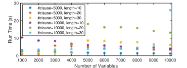
Figure 2: Experiment results from KB with different sizes.

To evaluate the proposed classifiers, we first conduct experiments on six real data sets, with results shown in Table 2.

Table 2: Experiment results (F₁ scores) with multiple data sets and several baseline algorithms.

Titanic Mushroom Nursery HIV-1 Bill Vehicle Tree 0.79 0.99 0.99 0.87 0.98 0.95 Direct 0.79 0.99 0.99 0.97 0.99 0.96 CART 0.82 0.99 0.99 0.94 0.99 0.98 MLP 0.81 0.99 0.99 0.73 0.98 0.96 Forest 0.82 0.99 1 0.98 0.99 0.98 SVM 0.78 0.99 0.99 0.99 0.99 0.97

For each data set, we measure the performance with the F₁ score, taken as the average of 50 runs for each data set. Our approaches are Tree (Algorithm 2) and Direct (Algorithm 3). We use CART (a decision tree algorithm), multi-layer perceptron (MLP) neural networks (with two hidden layers with 12 and 10 nodes, respectively), random forest (with 100 trees) and support vector machine as our comparison baselines. The six real data sets include the Titanic , Mushroom, Nursery and HIV-1 protease cleavage data sets from the UCI Machine Learning Repository (?), the UK parliament bill data set reported in (?) as well as an image data set for vehicle classification. For the Titanic data set, we used seven discrete features – ticket class, sex, age (discretized to 4 categories), number of siblings, number of parents, passenger fare (discretized to 3 categories), and port of embarkation. For the Mushroom data set, we used the first 11 features. For the multi-class data set Nursery, we randomly selected two classes and discarded others. For the Parliament bill, we used five features – House of Commons or House of Lords, type of bill, number of sponsors, bill subject, and final stages of the bill. The vehicle image data set contains 1635 images with 767 of them being cars and the rest busses and trucks. Feature extraction has been applied with 12 features created for each image. They are: number of pixels of the object, shape coefficient 1-5, mean and standard deviation of RGB channels. Each data set has been pre-processed such that the positive and the negative samples are balanced by randomly replicating samples in the smaller class. For all data set, the ratio between training and testing is 70% to 30%. Overall, we see that Direct gives satisfactory performance.

To evaluate our explanation approach, we first compare Direct with the state of the art Shapley Value based approach SHAP (?), using the Titantic and Mushroom data sets. The results are shown in Figure 3, with Figure 3(a)(b) showing the results from the Titantic data set and Figure 3(c)(d) from the Mushroom. Figure 3(a) shows the percentage of the same features suggested as explanations for different explanation lengths (i.e., $k=1,2,3,4,5$). For example, when $k=1$ (computing one-feature explanations), 75% of all instances have the same feature chosen as the explanation by both approaches. When $k=2$ (computing two-feature explanations), there are 72% and 25% instances found with the same 1 and 2 features, respectively. Figure 3(b) shows the percentage of each feature being selected as an explanation across all instances. We see that when $k=1$, ours and SHAP both suggest that feature 2 explains the classification result for over 70% instances. When $k=2$, the two approaches agree that feature 2 is an explanation while differing on the choice for the other feature.

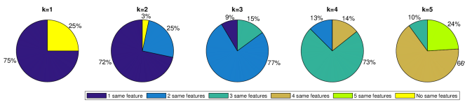
(a) The percentages of the same explanations suggested by Direct and Shapley over the Titantic data

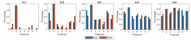
(b) The percentages of features serving as explanations suggested by Direct and Shapley over the Titantic data set

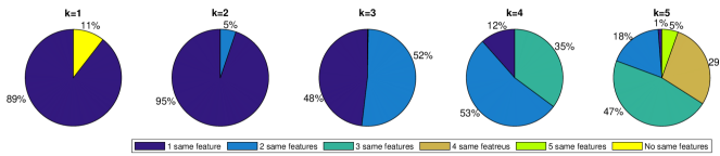
(c) The percentages of the same explanations suggested by Direct and Shapley over the Mushroom data set

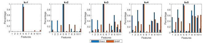
(d) The percentages of the same explanations suggested by Direct and Shapley over the Mushroom data set

Figure 3: Explanation results comparison.

Results presented in Figure 3 shows that our approach gives similar results to SHAP. As there is no explanation ground truth in these data sets, it is impossible to decide who gives “correct” explanations. To address this, we performed further experiments with synthetic data sets with known explanation ground truth. Specifically, we created four synthetic data sets of integer strings, Syn 10/4, Syn 10/8, Syn 12/4, and Syn 12/8, with the following rules. For each data set, we set a (random) seed string of the same length as strings in the data set from the same alphabet. For instance, for the “Syn 10/4” data set with 10 bits strings where each bit can take 4 possible values, 3232411132 is the seed. (Here, the size of the alphabet is 4. Each 10-bit string denotes a data instance with 10 features s.t. each feature takes its value from {1,2,3,4}.) A string $s$ in the data set is labelled positive iff $s$ match bits in the seed for exactly five places. E.g., 3133421242 is positive and 3133421232 is negative (it shares 6 bits as the seed rather than 5). For each string classified as positive, we compute a $k$-bit explanation. An explanation is correct iff the seed string has the same values for the bits identified as the explanation. The accuracy of an explanation is defined as the number of correct bits over the length of explanation. For instance, for $k=5$, we have

Query Explanation Seed Accuracy 3233112143 323–1-1– 3232411132 1.0 3244341112 -2—411-2 3232411132 0.8

The 2nd query contains an incorrect explanation 4. On our synthetic data sets with a 70% to 30% split on training and testing, the classification result is shown in Table 3 and the explanation accuracy for the Direct and SHAP approaches is shown in Table 4. This is an informative experiment as: (1) there is no “useless” feature in the data set as every feature (bit) could be decisive thus functions as part of an explanation as long as its value is the same as the feature in the seed; (2) the seed is the known ground truth for explanation comparison; (3) moreover, as shown in Table 3, these datasets represent non-trivial classification problems.

Table 3: Experiment results (F₁ scores) with synthetic data sets and several baseline algorithms.

Syn 10/4 Syn 10/8 Syn 12/4 Syn 12/8 Tree 0.71 0.78 0.62 0.70 Direct 0.92 0.95 0.89 0.94 CART 0.79 0.87 0.70 0.84 MLP 0.77 0.83 0.73 0.80 Forest 0.90 0.96 0.85 0.93 SVM 0.85 0.86 0.81 0.81

Table 4: Explanation accuracy on four syntactic data sets and various explanation lengths $k$.

$k=1$ $k=2$ $k=3$ $k=4$ $k=5$ 10/4 Direct 1 1 1 0.995 0.972 SHAP 1 1 0.996 0.993 0/962 10/8 Direct 1 1 0.997 0.980 0.976 SHAP 0.996 0.995 0.972 0.967 0.951 12/4 Direct 1 0.982 1 0.997 0.901 SHAP 0.993 0.980 0.973 0.942 0.856 12/4 Direct 1 1 0.998 0.975 0.964 SHAP 1 0.990 0.977 0.929 0.918

Table 3 shows that, similar to Table 2, the classification accuracy of our approach is competitive comparing to the baseline approaches. This further validates our approach for classification. Table 4 shows that although our approach (Direct) and SHAP both can identify part of the seed string from each query instances, hence computing correct explanations, ours gives higher accuracy across the board.

To demonstrate the effect of knowledge incorporation, we gradually add clauses drawn from sub-strings derived from the seed to the KB. The result is shown in Figure 4(a). Tested on the data set with string length 10, size of alphabet 4 with the Tree algorithm, we see that the classification performance improves as the number of true clauses inserted grows. To show that the knowledge incorporation is resilient to pollution, we insert clauses of a random length between 1 and 10 with a random probability to pollute the KB. As shown in Figure 4(b), for the same data set, the classification performance deteriorates gradually as the number of random clauses grows.

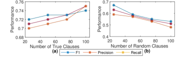
Figure 4: The plot on the left / right side shows classification results from KBs with true / random clauses inserted.

Related Work

Probabilistic logic programming, or ProbLog, (?) provides a means to do logic programming with probabilities. Our work differs from ProbLog in several ways. (1) ProbLog develops Logic Programming and uses grounded predicates with closed world assumption to allow negations whereas we use propositional clauses with classical negations; (2) ProbLog uses Sato’s distribution semantics and assumes all atomic variables, the variables not derived with Logic Programming, being independent whereas we use Nilsson’s probabilistic logic semantics and make no independence assumption. (3) ProbLog performs inference with weighted model counting, which is then solved with MAX-SAT, an NP-hard problem, whereas we use linear programming, which is polynomial.

Performing probabilistic logic inference with mathematical programming has been studied recently in (?) with its NonlInear Probabilistic Logic Solver (NILS) approach. Although in both works clauses with associated probabilities are turned into systems of equations, the two approaches differ significantly. NILS either assumes independence amongst its variables or expand probability of conjunctions as the product of the probability of a literal and some conditionals. Thus NILS produces non-linear systems and rely on gradient descent methods for finding solutions. Consequently, NILS is unsuitable for classification as the independence assumption does not hold between the class labels and feature values or, in general, values across different features. When independence cannot be assumed, systems constructed with NILS contains $k$th order equations with $2^{k}-1$ unknowns for each $k$ literal clauses. Such high order equations with high number unknowns are difficult to solve numerically. Comparing with NILS, the construction given in Definition 4 “hides” the complexity introduced by conditionals in NILS with inequalities and ensures polynomial complexity. Moreover, NILS does not tolerate inconsistency whereas our approach does.

More generally, developing intelligent system based on reasoning with KB has been explored in the past, see e.g., (?; ?). Some of the early works on learning KB from data use classical logic, e.g., (?) or default logic (?). A comprehensive review on combining logic and probability is beyond the scope of this section. For broader discussions on this topic, see e.g., (?) for probabilistic logic, (?) for weighted model counting, and (?) for probabilistic graphical models with logical structures. The problem of testing a KB’s consistency is known as the probabilistic satisfiability (PSAT) problem. Works dedicated to solving PSAT include (?; ?; ?). Since most of these compute exact solutions over consistent KBs by solving an NP problem, they are not suitable for classification.

In explainable machine learning, there has been significant interest in providing explanations for classifiers; see e.g., (?) for an overview. Works have been proposed to use simpler thus weaker classifiers to explain results from stronger ones, e.g., (?). Recent works on model-agnostic explainers (?; ?) focus on adding explanations to existing (black-box) classifiers. (?) use KB based classifiers to explain results obtained from MLP and random forests. LIME (?) augment the data with randomly generated samples close to the instance to be explained and then construct a simple thus explainable classifier to generate explanations. (?) works by decomposing a model’s predictions based on individual contributions of each feature. (?) explains Bayesian network classifiers by compiling naive Bayes and latent-tree classifiers into Ordered Decision Diagrams. (?) provides explanations for decision trees based on the game-theoretic Shapley values.

(?), (?) and (?) are some recent work on incorporating knowledge into machine learning. (?) contains a survey, categorising methods into four groups based on use of knowledge: (1) to prepare training samples, (2) to initialise the hypothesis or hypothesis space, (3) to alter the search objective and (4) to augment the search process. Our approach fundamentally differs from those as we represent knowledge in the same format as the model learned from data and reason with both uniformly.

Conclusion

We present a non-parametric classification technique that gives explanations to its predictions and supports knowledge incorporation. Our approach is based on approximating literal probabilities in probabilistic logic by solving linear systems corresponding to KBs, which are either directly learned from data or augmented with additional knowledge. Our linear program construction is efficient and our approaches tolerate inconsistency in a KB. As a stand-alone classifier, our approach matches or exceeds the performance of existing algorithms on both synthetic and non-synthetic data sets. At the same time, our approaches generate explanations in the form of “most decisive” features. Upon comparing with a state of the art Shapley Value based explanation method, SHAP, our approach finds similar explanation as SHAP on real data sets. On four synthetic data sets with known explanation ground truth, our approach is shown to be superior as it achieves higher accuracy. Overall, we envisage our approaches to be most useful for classification tasks where there exists knowledge to complement data and explanations are required to ensure usability.

There are four research directions that we plan to explore. Firstly, this work focuses on developing the underlying explainable classification techniques. We will apply techniques developed practical applications and perform user studies in the future. Secondly, we will study semantics for inconsistent KBs. Thirdly, we will study richer explanation generation with with (probabilistic) logic inference. Lastly, we would like to develop other suitable representations for knowledge incorporation.

References

- Alonso et al. 2018 Jose Alonso, Alejandro Ramos Soto, Ciro Castiello, and Corrado Mencar. Hybrid data-expert explainable beer style classifier. In Proc. of IJCAI-17 Workshop on Explainable AI, 2018.
- Apley and Zhu 2016 Daniel W. Apley and Jingyu Zhu. Visualizing the effects of predictor variables in black box supervised learning models, 2016.
- Bacchus 1990 F. Bacchus. Representing and Reasoning with Probabilistic Knowledge. MIT Press, Cambridge, MA, 1990.
- Berrar et al. 2019 Daniel Berrar, Philippe Lopes, and Werner Dubitzky. Incorporating domain knowledge in machine learning for soccer outcome prediction. Machine Learning, 108(1):97–126, Jan 2019.
- Biran and Cotton 2017 Or Biran and Courtenay V. Cotton. Explanation and justification in machine learning : A survey. In Proc. of IJCAI-17 Workshop on Explainable AI, 2017.
- Casella and Berger 2002 G. Casella and R.L. Berger. Statistical Inference. Duxbury advanced series in statistics and decision sciences. Thomson Learning, 2002.
- Chavira and Darwiche 2008 Mark Chavira and Adnan Darwiche. On probabilistic inference by weighted model counting. Artif. Intell., 172(6-7):772–799, 2008.
- Chiang et al. 2001 Ding-An Chiang, Wei Chen, Yi-Fan Wang, and Lain-Jinn Hwang. Rules generation from the decision tree. J. Inf. Sci. Eng., 17(2):325–339, 2001.
- Cozman and di Ianni 2015 Fabio G. Cozman and Lucas Fargoni di Ianni. Probabilistic satisfiability and coherence checking through integer programming. International Journal of Approximate Reasoning, 58:57 – 70, 2015. Special Issue of the Twelfth European Conference on Symbolic and Quantitative Approaches to Reasoning with Uncertainty (ECSQARU 2013).
- Doran et al. 2017 D. Doran, S. Schulz, and T. R. Besold. What does explainable AI really mean? A new conceptualization of perspectives. CoRR, abs/1710.00794, 2017.
- Dua and Karra Taniskidou 2017 Dheeru Dua and Efi Karra Taniskidou. UCI machine learning repository, 2017.
- Fierens et al. 2015 Daan Fierens, Guy Van den Broeck, Joris Renkens, Dimitar Sht. Shterionov, Bernd Gutmann, Ingo Thon, Gerda Janssens, and Luc De Raedt. Inference and learning in probabilistic logic programs using weighted boolean formulas. TPLP, 15(3):358–401, 2015.
- Finger and Bona 2011 Marcelo Finger and Glauber De Bona. Probabilistic satisfiability: Logic-based algorithms and phase transition. In IJCAI 2011, Proceedings of the 22nd International Joint Conference on Artificial Intelligence, Barcelona, Catalonia, Spain, July 16-22, 2011, pages 528–533, 2011.
- Fisher et al. 2018 A. Fisher, C. Rudin, and F Dominici. All Models are Wrong but many are Useful: Variable Importance for Black-Box, Proprietary, or Misspecified Prediction Models, using Model Class Reliance. arXiv e-prints, page arXiv:1801.01489, Jan 2018.
- Féraud and Clérot 2002 Raphael Féraud and Fabrice Clérot. A methodology to explain neural network classification. Neural Networks, 15(2):237 – 246, 2002.
- Georgakopoulos et al. 1988 George Georgakopoulos, Dimitris Kavvadias, and Christos H Papadimitriou. Probabilistic satisfiability. Journal of Complexity, 4(1):1 – 11, 1988.
- Gogate and Domingos 2016 Vibhav Gogate and Pedro M. Domingos. Probabilistic theorem proving. Commun. ACM, 59(7):107–115, 2016.
- Henderson et al. 2020 T.C. Henderson, R. Simmons, B. Serbinowski, M. Cline, D. Sacharny, X. Fan, and A. Mitiche. Probabilistic sentence satisfiability: An approach to psat. Artificial Intelligence, 278:103199, 2020.
- Khardon and Roth 1994 Roni Khardon and Dan Roth. Learning to reason. In Proceedings of the 12th National Conference on Artificial Intelligence, Seattle, WA, USA, July 31 - August 4, 1994, Volume 1., pages 682–687, 1994.
- Lundberg and Lee 2017 Scott M. Lundberg and Su-In Lee. A unified approach to interpreting model predictions. In Proc. of NIPS, pages 4768–4777, 2017.
- Lundberg et al. 2020 Scott M. Lundberg, Gabriel Erion, Hugh Chen, Alex DeGrave, Jordan M. Prukin, Bala Nair, Bonit Katz, Jonathan Himmelfarb, Nisha Bansal, and Su-In Lee. From local explanations to golbal understanding with explainable ai for trees. Nature machine intelligence, 2(1):56–67, 2020.
- Mashayekhi and Gras 2017 Morteza Mashayekhi and Robin Gras. Rule extraction from decision trees ensembles: New algorithms based on heuristic search and sparse group lasso methods. International Journal of Information Technology & Decision Making, 16(06):1707–1727, 2017.
- McCarthy 1968 John McCarthy. Programs with common sense. In Semantic Information Processing, pages 403–418. MIT Press, 1968.
- Molnar 2019 Christoph Molnar. Interpretable Machine Learning, A Guide for Making Black Box Models Explainable. 2019. https://christophm.github.io/interpretable-ml-book/.
- Nilsson 1986 Nils J. Nilsson. Probabilistic logic. Artificial Intelligence, 28(1):71–87, 1986.
- Nilsson 1991 N. Nilsson. Logic and artificial intelligence. Artif. Intell., 47(1-3):31–56, 1991.
- Quinlan 1987 J. R. Quinlan. Generating production rules from decision trees. In Proc of IJCAI, pages 304–307, 1987.
- Ribeiro et al. 2016 Marco Túlio Ribeiro, Sameer Singh, and Carlos Guestrin. ”why should I trust you?”: Explaining the predictions of any classifier. In Proc. of SIGKDD, pages 1135–1144, 2016.
- Ribeiro et al. 2018 Marco Túlio Ribeiro, Sameer Singh, and Carlos Guestrin. Anchors: High-precision model-agnostic explanations. In Proc of AAAI-18, pages 1527–1535, 2018.
- Robnik-Šikonja and Kononenko 2008 M. Robnik-Šikonja and I. Kononenko. Explaining classifications for individual instances. IEEE Transactions on Knowledge and Data Engineering, 20(5):589–600, May 2008.
- Roth 1996 Dan Roth. Learning in order to reason: The approach. In SOFSEM ’96: Theory and Practice of Informatics, 23rd Seminar on Current Trends in Theory and Practice of Informatics, Milovy, Czech Republic, November 23-30, 1996, Proceedings, pages 113–124, 1996.
- Rudin 2019 Cynthia Rudin. Stop explaining black box machine learning models for high stakes decisions and use interpretable models instead. Nature Machine Intelligence, 1:206–215, May 2019.
- Sachan et al. 2018 Mrinmaya Sachan, Kumar Avinava Dubey, Tom M. Mitchell, Dan Roth, and Eric P. Xing. Learning pipelines with limited data and domain knowledge: A study in parsing physics problems. In Proc. of NIPS, pages 140–151, 2018.
- Shih et al. 2018 Andy Shih, Arthur Choi, and Adnan Darwiche. A symbolic approach to explaining bayesian network classifiers. In Proc. of IJCAI, pages 5103–5111, 2018.
- Vo et al. 2017 Khuong Vo, Dang Pham, Mao Nguyen, Trung Mai, and Tho Quan. Combination of domain knowledge and deep learning for sentiment analysis. In Somnuk Phon-Amnuaisuk, Swee-Peng Ang, and Soo-Young Lee, editors, Multi-disciplinary Trends in Artificial Intelligence, pages 162–173, Cham, 2017. Springer International Publishing.
- Štrumbelj and Kononenko 2014 Erik Štrumbelj and Igor Kononenko. Explaining prediction models and individual predictions with feature contributions. Knowledge and Information System, 41(3):647–665, December 2014.
- Yang et al. 2017 H. Yang, C. Rudin, and M. Seltzer. Scalable bayesian rule lists. In Proc. of ICML, pages 3921–3930, 2017.
- Čyras et al. 2019 Kristijonas Čyras, David Birch, Yike Guo, Francesca Toni, Rajvinder Dulay, Sally Turvey, Daniel Greenberg, and Tharindi Hapuarachchi. Explanations by arbitrated argumentative dispute. Expert Systems with Applications, 127:141 – 156, 2019.
- Yu 2007 Ting Yu. Incorporating Prior Domain Knowledge into Inductive Machine Learning. PhD thesis, University of Technology Sydney, Sydney, Australia, 2007.
- Zhao and Hastie 2019 Qingyuan Zhao and Trevor Hastie. Causal interpretations of black-box models. Journal of Business & Economic Statistics, 0(0):1–10, 2019.