Encoding Linear Constraints into SAT

Abstract

Linear integer constraints are one of the most important constraints in combinatorial problems since they are commonly found in many practical applications. Typically, encodings to Boolean satisfiability (SAT) format of conjunctive normal form perform poorly in problems with these constraints in comparison with SAT modulo theories (SMT), lazy clause generation (LCG) or mixed integer programming (MIP) solvers.

In this paper we explore and categorize SAT encodings for linear integer constraints. We define new SAT encodings based on multi-valued decision diagrams, and sorting networks. We compare different SAT encodings of linear constraints and demonstrate where one may be preferable to another. We also compare SAT encodings against other solving methods and show they can be better than linear integer (MIP) solvers and sometimes better than LCG/SMT solvers on appropriate problems. Combining the new encoding with lazy decomposition, which during runtime only encodes constraints that are important to the solving process that occurs, gives the best option for many highly combinatorial problems involving linear constraints.

1 Introduction

In this paper we study linear integer (LI) constraints, that is, constraints of the form $a_{1}x_{1}+\cdots+a_{n}x_{n}\;\#\;a_{0}$, where the $a_{i}$ are integer given values, the $x_{i}$ are finite-domain integer variables, and the relation operator $\#$ belongs to $\{<,>,\leqslant,\geqslant,=\}$.

Linear integer constraints appear in almost every combinatorial problem, including scheduling, planning and software verification, and, therefore, many different Boolean satisfiability (SAT) encodings (see e.g. ?, ?), SAT Modulo Theory (SMT) theory solvers (?, ?), and propagators (?) for Constraint Programming (CP) solvers (?) have been suggested for handling them.

In this paper we survey existing methods for encoding special cases of linear constraints, in particular pseudo-Boolean (PB) constraints (where $x_{1},\ldots,x_{n}$ are Boolean (or 0-1) variables), and cardinality constraints (CC) (where, moreover, $a_{i}=1,1\leq i\leq n$). We then show how these can be extended to encode general linear integer constraints.

The first method proposed here roughly consists in encoding a linear integer constraint into a Reduced Ordered Multi-valued Decision Diagram (MDD for short), and then decomposing the MDD to SAT. There are different reasons for choosing this approach: firstly, most state-of-the-art encoding methods define one auxiliary variable for every different possible value of the partial sum $s_{i}=a_{i}x_{i}+a_{i+1}x_{i+1}+\cdots+a_{n}x_{n}$. However, some values of the partial sums may be equivalent in the constraint. For example, the expression $s_{2}=2x_{2}+5x_{3}$ with $x_{2}\in[0,2]$ and $x_{3}\in[0,3]$ cannot take the value 13 and hence the constraints $s_{2}\leq 12$ and $s_{2}\leq 13$ are equivalent, and hence we don’t need to encode both possible partial sum results. With MDDs, due to the reduction process, we can identify these situations, and encode all these indistinguishable values with a single variable, producing a more compact encoding.

Secondly, BDDs are one of the best methods for encoding pseudo-Boolean constraints into SAT by ? (?), and MDDs seems the natural tool to generalize the pseudo-Boolean encoding.

The second method uses sorting networks to encode the LI constraints. The encoding is a generalization of the methods by ? (?) and by ? (?) that have good propagation properties and better asymptotic size than the BDD/MDD encodings.

The goal of these encodings is not for use in arbitrary problems involving linear integer constraints. In fact, a specific linear integer (MIP) solver or CP or SMT solver will usually outperform any SAT encoding in problems with many more linear integer constraints than Boolean clauses.

Nevertheless, a fairly common kind of combinatorial problem consists mainly of Boolean variables and clauses, but also a few integer variables and LI constraints. Among these problems, an important class correspond to SAT problems with a linear integer optimization function. In these cases, SAT solvers are the optimal tool for solving the problem, but a good encoding for the linear integer constraints is needed to make the optimization effective. Therefore, in these problems the decompositions presented here can make a significant difference.

Note, however, that decomposing the constraint may not always be the best option. In some cases the encoding might produce a large number of variables and clauses, transforming an easy problem for a CP solver into a huge SAT problem. In some other cases, nevertheless, the auxiliary variables may give an exponential reduction of the search space. Lazy decomposition (?, ?) is a hybrid approach that has been successfully used to handle this issue for cardinality and pseudo-Boolean constraints. Here, we show that it also can be applied successfully on linear integer constraints.

The methods proposed here use the order encoding (?, ?) for representing the integer variables. For some LI constraints, however, the domains of the integer variables are too large to effectively use the order encoding. We also propose a new alternative method for encoding linear integer constraints using a logarithmic encoding of the integer variables.

In summary, the contributions of this paper are:

• A precise definition of correct SAT encodings of constraints over non-Boolean variables and the consistency maintained by such a SAT encoding.

• A new encoding (MDD) for LI constraints using MDDs that can outperform other state-of-the-art encodings.

• A new encoding for Monotonic MDDs into CNF.

• A new encoding (SN) for LI constraints using sorting networks that can outperform other state-of-the-art encodings.

• A new proof of consistency of direct sorting network encodings of LI (that is, without using “tare” trick to adjust the right hand side $a_{0}$ to be a power of 2). This is an open question in the MiniSAT+ paper (?).

• An alternative encoding (BDD-Dec) for LI constraints for large constraints or variables with huge domains.

• An extensive experimental comparison of our methods with respect to other decompositions to SAT and other solvers. A total of 14 methods are compared, on more than 5500 benchmarks, both industrial and crafted.

The paper is organized as follows. First in Section 2 we introduce SAT solvers, encodings of integer variables, and how to transform linear constraints to a standard form. Next in Section 3, because they are useful also for encoding LI constraints, we survey methods for encoding cardinality constraints into CNF. Then in Section 4, because methods for encoding linear constraints are typically extensions of methods for encoding PB constraints, we review various methods for encoding pseudo-Boolean constraints into CNF.

In Section 5 we come to the core of the paper, which examines various methods for encoding general linear integer constraints. We first concentrate on encodings using the order encoding of integers. In Section 5.2 we introduce a simplification of LI constraints (and PB constraints) that improves on their encoding (and also requires the use LI encodings for what were originally PB constraints). In Section 5.3 we define how to encode LI constraints using multi-valued decision diagrams (MDDs). In Section 5.4 we define how to encode LI constraints using sorting networks. In Section 5.5 we review the only existing encoding of general linear constraints to SAT that maintains domain consistency, based on using partial sums. In Section 5.6 we review the existing encodings of general linear constraints to SAT based on logarithmic encodings of integers, and define a new approach BDD-Dec. In Section 6 we give detailed experiments investigating the different encodings, and also compare them against other solving techniques. Finally in Section 7 we conclude.

Figure 1 gives an overview the different translations and contributions in this paper. The graph shows a selection of different translations from LI and PB constraints to intermediate data structures in focus. The arrows are annotated by the respective publications and Sections. At the root we have the Linear constraint and its decomposition to the PB constraints by various methods. A second set of arrows connects the LI constraints with the data structures directly.

Figure 1: An overview of various methods to encode LI and PB constraints. The majority of the encodings of LI translate first to PB and use existing encodings thereof, whereas others translate directly. The terminals symbolize the basic building structure of the translation.

We summarize the state of the art in CC, PB and LI encodings of the constraint $a_{1}x_{1}+a_{2}x_{2}+\cdots+a_{n}x_{n}\leq a_{0}$ where the number of variables in the LI is $n$, $a_{0}$ is the right hand side coefficient, $a_{\max}$ is the largest left hand side coefficient, and $d$ is the the size of the largest integer variable domain, in Table 1. The table shows the basis of construction method using Adders, using Totalizers, using sorting networks (SN), using cardinality networks (CN), using BDDs, using watchdogs (GPW and LPW), and for the general linear (LI) encodings the named encoding. It gives a reference for the method, and a page where it is discussed. It then shows the asymptotic size of the encoding and the consistency maintained by unit propagation on the encoding (see Section 2.2), where — indicates no consistency. Note that any method with a coefficient $a_{0}$ outside the $\log$ is exponential in size, the remainder are polynomial.

Table 1: Summary of different encodings for CC, PB and LI constraints.

Cons	Construction	Reference	Page	# Clauses	Consistency
CC	Adder	(?)	3.1	$O(n)$	—
CC	Totalizer	(?)	3.2.1	$O(n^{2})$	Domain
CC	SN	(?)	3.2.2	$O(n\log^{2}(n))$	Domain
CC	CN	(?)	9	$O(n\log^{2}(a_{0}))$	Domain
CC	CN	(?)	9	$O(n\log^{2}(a_{0}))$	Domain
PB	Adder	(?)	11	$O(n\log(a_{0}))$	—
PB	Adder	(?)	4.1	$O(n\log(a_{0}))$	—
PB	BDD	(?)	7	$O(na_{0})$ 6/Node	Domain
PB	BDD	(?)	4.3	$O(na_{0})$ 4/Node	Domain
PB	BDD	(?)	7	$O(na_{0})$ 2/Node	Domain
PB	SN	(?)	LABEL:eensn	$O(n\log(a_{\max})\log^{2}(n\log(a_{\max})))$	Consistent
PB	GPW	(?)	4.2	$O(n^{2}\log^{2}(n)\log(a_{\max}))$	Consistent
PB	LPW	(?)	4.2	$O(n^{3}\log^{2}(n)\log(a_{\max}))$	Domain
PB	SN	(?)	14	$O(n^{2}\log^{2}(n)\log(a_{\max}))$	Domain
LI	Adder	(?)	5.6.1	$O(n\log(a_{0}))$	—
LI	SN	(?)		$O(nda_{0})$	—
LI	SN	5.4	5.4	$O(n\log(d)\log(n)\log(a_{\max}))$	Consistent
LI	BDD	(?)	39	$O(n\log(d)\log(a_{0}))$	—
LI	BDD-Dec	5.6	5.6	$O(n^{2}\log(d)\log(a_{\max}))$	—
LI	Support	(?)	5.5	$O(nda_{0})$	Domain
LI	MDD	5.3	5.3	$O(nda_{0})$	Domain

2 Propagation and Encodings

In this section we introduce the concepts of variables, domains, constraints, propagators and encodings into SAT. Mostly, the terminology we use is standard. The exception is the encodings into SAT: unfortunately, there is no standard definition for this.

In fact, most papers do not define what is an encoding or what it means for an encoding to be consistent. In the case of encodings of constraints of Boolean variables this is not a problem, but, in general, when dealing with integer variables some encodings cannot represent all possible domains. In this case, the meaning of consistency is not clear. In this section we provide a precise definition of encodings into SAT for both Boolean and integer variables. With this definition, the concept of consistency can naturally be extended to encodings.

2.1 Domains, Constraints and Propagators

We use $[l,u]$ to denote the interval of integers $\{d~{}|~{}l\leq d\leq u\}$. Let ${\cal X}$ be a fixed set of variables. A domain $D$ is a complete mapping from ${\cal X}$ to a set of subsets of finite set of integers. Given a domain $D$, and a variable $x\in{\cal X}$, the domain of the variable $x$ is the set $D(x)\subset\mathbb{Z}$. In the following, let us fix an initial domain $D$.

A false domain $D$ is one where $D(x)=\emptyset$ for some $x\in{\cal X}$. Let $\oslash$ be the false domain where $\oslash(x)=\emptyset,\forall x\in{\cal X}$. A domain $D_{1}$ is stronger than a domain $D_{2}$, written $D_{1}\sqsubseteq D_{2}$, if $D_{1}(x)\subseteq D_{2}(x)$ for all $x\in{\cal X}$. Given the domains $D_{1}$ and $D_{2}$, the domain $D_{1}\sqcap D_{2}$ is the domain such that $D_{1}\sqcap D_{2}(x)=D_{1}(x)\cap D_{2}(x)$ for all $x\in{\cal X}$. In this paper we assume that the initial domain is convex, i.e., that the domain of every variable $x\in{\cal X}$ is an interval. A complete assignment is a domain $D^{\prime}$ such that $|D^{\prime}(x)|=1$ for all $x\in{\cal X}$.

A constraint $c$ over the variables $x_{1},x_{2},\ldots,x_{n}\in{\cal X}$ is a subset of the Cartesian product $D(x_{1})\times D(x_{2})\times\cdots\times D(x_{n})$. A complete assignment $D^{\prime}$ satisfies the constraint $c$ if $D^{\prime}(x_{i})=\{d_{i}\},1\leq i\leq n$ and $(d_{1},d_{2},\ldots,d_{n})\in c$. The solutions of a constraint $c$, denoted as $\text{solns}(c)$, are the set of complete assignments that satisfy $c$. A constraint $c$ is satisfiable on the domain $D_{1}$ if there is a complete assignment $D_{2}\sqsubseteq D_{1}$ that satisfies $c$. Otherwise, it is unsatisfiable on $D_{1}$.

Given a constraint $c$, a propagator $f$ is a monotonically decreasing function from domains to domains such that $f(D^{\prime})\sqsubseteq D^{\prime}$ for all domain $D^{\prime}$; a monotonically decreasing function is such that if $D_{1}\sqsubseteq D_{2}$ then $f(D_{1})\sqsubseteq f(D_{2})$. A propagator $f$ is correct if for all domains $D^{\prime}$, $\{\text{solns}(c)\ |\ \text{solns}(c)\sqsubseteq D^{\prime}\}=\{\text{solns}(c)\ |\ \text{solns}(c)\sqsubseteq f(D^{\prime})\}$.

Constraint Programming (CP) solvers solve problems by maintaining a domain $D$, and reducing the domain using a propagator for each constraint $c$ in the problem. When propagation can make no further reduction, the solver splits the problem into two, typically by splitting the domain of a variable in two disjoint parts, and examines each subproblem in turn.

2.2 Consistency

The identity propagator, $id(D)=D$, is correct for any constraint. In practice we want propagators to enforce some stronger condition than correctness. The usual conditions of interest are:

consistent

A propagator $f$ is consistent for $c$ if, given any domain $D^{\prime}$ where $c$ is unsatisfiable on it, $f(D^{\prime})$ is a false domain. That is it detects when the constraint can no longer be satisfied by the domain.

domain consistent

A propagator $f$ is domain consistent for $c$ if, given any domain $D_{1}$, for all $x\in{\cal X}$ and $d\in f(D_{1})(x)$, $c$ is satisfiable on

$$D_{2}=\begin{cases}x^{\prime}\mapsto f(D_{1})(x^{\prime})&\mbox{if }x^{\prime}\neq x\\ x^{\prime}\mapsto\{d\}&\mbox{if }x^{\prime}=x\end{cases}$$

A domain consistent propagator infers the maximum possible information, representable in the domain, from the constraint.

bounds consistent

A propagator $f$ is bounds consistent for $c$ if, given any domain $D_{1}$, for all $x\in{\cal X}$ with $f(D_{1})$ not a false domain, $c$ is satisfiable on

$$D_{2}=\begin{cases}x^{\prime}\mapsto[\min f(D_{1})(x^{\prime}),\max f(D_{1})(x^{\prime})]&\mbox{if }x^{\prime}\neq x\\ x^{\prime}\mapsto\{l\}&\mbox{if }x^{\prime}=x\end{cases}$$

and

$$D_{3}=\begin{cases}x^{\prime}\mapsto[\min f(D_{1})(x^{\prime}),\max f(D_{1})(x^{\prime})]&\mbox{if }x^{\prime}\neq x\\ x^{\prime}\mapsto\{u\}&\mbox{if }x^{\prime}=x\end{cases}$$

where $l=\min f(D_{1})(x)$ and $u=\max f(D_{1})(x)$. A bounds consistent propagator enforces that the upper and lower bounds of each variable appear in some solution to the constraint.

Example 1.

Given $x_{1},x_{2},x_{3}\in{\cal X}$ with initial domain $x_{1}\in[0,4]$, $x_{2}\in[0,2]$ and $x_{3}\in[0,3]$, let us consider the constraint $c:3x_{1}+2x_{2}+5x_{3}\leqslant 15$. The propagator $f$ defined by

$$f(D_{1})=\begin{cases}D_{1}&\mbox{if }3\min D_{1}(x_{1})+2\min D_{1}(x_{2})+5\min D_{1}(x_{3})\leqslant 15\\ \oslash&\mbox{otherwise}\end{cases}$$

is correct, since if $\{\text{solns}(c)\sqsubset D_{1}\}\neq\emptyset$, then $f(D_{1})=D_{1}$. It is consistent since if $f(D_{1})\neq\oslash$, then $\{x_{i}=\min D_{1}(x_{i})\ |\ i=1,2,3\}$ is a solution of $c$. However, $f$ is not bounds consistent, since given $D_{1}=\{x_{1}\in[0,4],\ x_{2}\in[0,2],\ x_{3}\in[3,3]\}$, $f(D_{1})=D_{1}$, but $c$ is unsatisfiable in $D_{3}=\{x_{1}\in[4,4],\ x_{2}\in[0,2],\ x_{3}\in[3,3]\}$. In the same way, the propagator is not domain consistent.

2.3 SAT Solving

Let ${\cal Y}=\{y_{1},y_{2},\ldots\}$ be a fixed set of propositional variables. If $y\in{\cal Y}$ then $y$ and $\neg y$ are positive and negative literals, respectively. The negation of a literal $l$, written $\neg l$, denotes $\neg y$ if $l$ is $y$, and $y$ if $l$ is $\neg y$. A clause is a disjunction of literals $\neg y_{1}\lor\cdots\lor\neg y_{p}\lor y_{p+1}\lor\cdots\lor y_{n}$, sometimes written as $y_{1}\land\cdots\land y_{p}\rightarrow y_{p+1}\lor\cdots\lor y_{n}$. A CNF formula is a conjunction of clauses. Clauses and CNF formulas can be seen as constraints as defined in the previous section.

A partial assignment $A$ is a set of literals such that $\{y,\neg y\}\not\subseteq A$ for any $y\in{\cal Y}$, i.e., no contradictory literals appear. A literal $l$ is true in $A$ if $l\in A$, is false in $A$ if $\neg{l}\in A$, and is undefined in $A$ otherwise. True, false or undefined is the polarity of the literal $l$. A non-empty domain $D$ on ${\cal Y}$ defines a partial assignment $A$ in the obvious way: if $D(y)=\{0\}$, then $\neg y\in A$; if $D(y)=\{1\}$, then $y\in A$; and if $D(y)=\{0,1\}$, $y$ is undefined in $A$.

Given a CNF formula $F$, unit propagation is the propagator defined as following: given an assignment $A$, it finds a clause in $F$ such that all its literals are false in $A$ except one, say $l$, which is undefined, add $l$ to $A$ and repeat the process until reaching a fix-point.

We assume a basic model of a propagation based SAT solver which captures the majority of SAT solvers: A system that decides whether a formula has a model by extending partial assignments through deciding on unassigned variables and reasoning via unit propagation. See e.g. the work by ? (?) for more details. More advance concepts such as heuristics or conflict clause learning are not explicitly needed for our investigation. In our analysis of encodings we do not consider SAT solvers that follow other paradigms, for instance local search.

2.4 Encoding of Integer Variables

SAT solvers cannot directly deal with non-propositional variables. Therefore, to tackle a general problem with SAT solvers, the non-propositional variables must be transformed into propositional ones. This process is called encoding the integer variables into SAT.

Given a set of integer variables $\cal X$ with initial domain $D$, an encoding of ${\cal X}$ into SAT is a set of propositional variables ${\cal Y}$, a CNF formula $F$ and a monotonically decreasing function $e$ between domains of $\cal X$ and partial assignments on ${\cal Y}$ such that:

• If $D^{\prime}$ is empty for some $x\in{\cal X}$, then $e(D^{\prime})$ cannot satisfy $F$.

• If $D^{\prime}$ is a complete assignment of $\cal X$, $e(D^{\prime})$ is a complete assignment of ${\cal Y}$ and it satisfies $F$.

• The restriction of $e$ to complete assignments is injective.

Given $({\cal Y},F,e)$ an encoding of a set of integer variables $\cal X$, we can define a monotonically decreasing function $e^{-1}$ between partial assignments of $\cal Y$ to domains on ${\cal X}$ as

$$e^{-1}(A)=\bigsqcap{\{D^{\prime}\ |\ e(D^{\prime})\subseteq A\}}.$$

Notice that $e^{-1}(e(D^{\prime}))=D^{\prime}$. Also notice that $e^{-1}$ is the inverse of the restriction of $e$ to complete assignments of ${\cal X}$.

Here we consider encodings of a single integer variable: these encodings can be extended to sets of integer variables in the obvious way.

There are different methods to encode finite domain variables to SAT that maintain different levels of consistency. A methodical introduction to this topic is given by ? (?) and ? (?). In case of integer variables for our investigation we focus on the order and the logarithmic encoding that we will properly define in this section. We will not consider the direct encoding since it performs badly with LI constraints (e.g. ?): it requires a huge number of clauses even in the simplest LI constraints. Logarithmic encoding produces the most compact encodings of LI constraints at the expense of propagation strength. Order encoding produces the smallest encodings among those with good propagation properties.

Let $x$ be an integer variable with initial domain $[a,b]$. The order encoding (?, ?) - sometimes called the ladder or regular encoding - introduces Boolean variables $y^{i}$ for $a+1\leqslant i\leqslant b$. A variable $y^{i}$ is true iff $x\geqslant i$. The encoding also introduces the clauses $y^{i+1}\rightarrow y^{i}$ for $a+1\leqslant i<b$. In the following, we denote $\operatorname{Order-Encoding}(x):=[y^{a+1},y^{a+2},\ldots,y^{b}]$. Given a domain $D^{\prime}\subseteq[a,b]$ of $x$, let us define $l=\min D^{\prime}$ and $u=\max D^{\prime}$. Then, $e(D^{\prime})=\{y^{i}\ |\ i\geq l\}\cup\{\neg y^{i}\ |\ i\geq u+1\}$.

Given $x$ be an integer variable with initial domain $[0,2^{n}-1]$. The logarithmic encoding introduces only $n$ variables $y_{b}^{i}$ which codify the binary representation of the value of $x$, as $x=\sum_{i=0}^{n}2^{i}y_{b}^{i}$. In the following, we denote $\operatorname{Logarithmic-Encoding}(x):=[y_{b}^{0},y_{b}^{1},\ldots,y_{b}^{n-1}$. It is a more compact encoding, but it usually gives poor propagation performance. Given a domain $D^{\prime}$ over ${\cal X}=\{x\}$ where $D^{\prime}(x)\subseteq[0,2^{n}-1]$, $e(D^{\prime})=\{y_{b}^{i}\ |\ \forall v\in D^{\prime}(x)\,v/2^{i}\equiv 1\ (\textrm{mod}~{}2)\}\cup\{\neg y_{b}^{i}\ |\ \forall v\in D^{\prime}(x),v/2^{i}\equiv 0\ (\textrm{mod}~{}2)\}$.

We will only be interested in encoding linear constraints with variables with initial domain $[0,d]$ (see Section 2.6). To generate the logarithmic encoding for such a variable with $d\neq 2^{n}-1$. We generate the encoding for an integer with initial domain $[0,2^{m}-1]$ where $m=\lceil\log(d+1)\rceil$. We then add constraints encoding $x\leq d$ as the lexicographic ordering constraint $[y^{m-1}_{b},y^{m-2}_{b},\ldots,y^{0}_{b}]\leq[bit(m-1,d),bit(m-2,d),\ldots,bit(0,d)]$ where $bit(i,d)$ returns the $i^{th}$ bit in the unsigned encoding of positive integer $d$. The clauses are

$$\bigwedge_{i=0..m-1,bit(i,d)=0}((\bigvee_{j=i+1..m-1,bit(i,d)=0}y_{b}^{j})\vee(\bigvee_{j=i+1..m-1,bit(i,d)=1}\neg y_{b}^{j})\vee\neg y_{b}^{i})$$

which encode that if the first $m-i-2$ elements in the list are equal, and the $i^{th}$ bit of $d$ is a 0, then $\neg y_{i}$ must hold.

Example 2.

Consider encoding a variable $x$ taking values from $[0,9]$. Then $m=4$ and the bits of $d=9$ are $bit(3,d)=1$, $bit(2,d)=0$, $bit(1,d)=0$, $bit(0,d)=1$. We generate Boolean encoding variables $[y_{b}^{0},y_{b}^{1},y^{2}_{b},y^{3}_{b}]$. We encode $x\leq 9$ using the clauses $\neg y_{b}^{3}\vee\neg y_{b}^{2}$, $\neg y_{b}^{3}\vee y_{b}^{2}\vee\neg y_{b}^{1}$. Notice these clauses can be simplified (by Krom subsumption) to $\neg y_{b}^{3}\vee\neg y_{b}^{2}$, $\neg y_{b}^{3}\vee\neg y_{b}^{1}$.

2.5 Encoding constraints into SAT

In the same way, SAT solvers cannot directly deal with general constraints, so they must be encoded as well. In this section we explain what is an encoding of a general constraint into SAT.

Let $D$ be a domain on the variables $\cal X$, and let $c$ be a constraint on ${\cal X}$. Let $({\cal Y},F,e)$ be an encoding of $\cal X$. An encoding of $c$ into SAT is a set of propositional variables ${\cal Y}_{c}\supseteq{\cal Y}$ and a formula $F_{c}$ such that given $D^{\prime}$ a complete assignment on $\cal X$, $D^{\prime}$ satisfies $c$ if and only if $F_{c}$ is satisfiable on $e(D^{\prime})$.

Given an encoding of a constraint $c$ into SAT, unit propagation defines a propagator of $c$:

Proposition 3.

Let $D$ be a domain on the variables $\cal X$, and let $c$ be a constraint on $\cal X$. Let $({\cal Y},F,e)$ be an encoding of $\cal X$ and $({\cal Y}_{c},F_{c})$ an encoding of $c$. Then $D_{1}\mapsto D_{1}\sqcap(e^{-1}\circ\pi_{|{\cal Y}}\circ\textrm{up}_{F_{c}}\circ e)(D_{1})$ is a correct propagator of $c$, where $\pi_{|{\cal Y}}$ is the projection from ${\cal Y}_{c}$ to $\cal Y$ and $\textrm{up}_{F_{c}}$ is the unit propagation on $F_{c}$.

Since an encoding of a constraint into SAT defines a propagator of that constraint, the notions of consistency, bound consistency and domain consistency can be extended to encodings: an encoding is consistent/bound consistent/domain consistent if the propagator it defines is.

Example 4.

Let us consider again the constraint $c:3x_{1}+2x_{2}+5x_{3}\leqslant 15$, where $x_{1}\in[0,4]$, $x_{2}\in[0,2]$ and $x_{3}\in[0,3]$. Let $({\cal Y},F,e)$ be the order encoding of $\cal X$. We define

$$F_{c}=\bigwedge\left\{\neg y_{1}^{i}\vee\neg y_{2}^{j}\vee\neg y_{3}^{k}\ |\ i\in[0,4],j\in[0,2],k\in[0,5],3i+2j+5k>15\right\}\wedge y_{1}^{0}\wedge y_{2}^{0}\wedge y_{3}^{0}$$

and ${\cal Y}_{c}={\cal Y}\cup\{y_{1}^{0},y_{2}^{0},y_{3}^{0}\}$. Then, $({\cal Y}_{c},F_{c})$ is an encoding of $c$.

Let $f=e^{-1}\circ\pi_{|{\cal Y}}\circ\textrm{up}_{F_{c}}\circ e$ be the propagator defined by unit propagation and $F_{c}$. Given $D_{1}=\{x_{1}\mapsto\{1,2,3\},x_{2}\mapsto\{0,2\},x_{3}\mapsto\{2,3\}\}$,

$$e(D_{1})=\{y_{1}^{1},\neg y_{1}^{4},y_{3}^{1},y_{3}^{2}\}.$$

Unit propagation propagates $y_{1}^{0},y_{2}^{0},y_{3}^{0},\neg y_{1}^{2}$ (due to clause $\neg y_{1}^{2}\vee\neg y_{2}^{0}\vee\neg y_{3}^{2}$), $\neg y_{1}^{3}$ (due to clause $\neg y_{1}^{3}\vee\neg y_{2}^{0}\vee\neg y_{3}^{2}$)and $\neg y_{2}^{2}$ (due to clause $\neg y_{1}^{1}\vee\neg y_{2}^{2}\vee\neg y_{3}^{2}$). So

$$\textrm{up}_{F_{c}}(e(D_{1}))=\{y_{1}^{0},y_{1}^{1},\neg y_{1}^{2},\neg y_{1}^{3},\neg y_{1}^{4},y_{2}^{0},\neg y_{2}^{2},y_{3}^{0},y_{3}^{1},y_{3}^{2}\}.$$

Therefore,

$$\pi_{|{\cal Y}}(\textrm{up}_{F_{c}}(e(D_{1})))=\{y_{1}^{1},\neg y_{1}^{2},\neg y_{1}^{3},\neg y_{1}^{4},\neg y_{2}^{2},y_{3}^{1},y_{3}^{2}\},$$

so

$$e^{-1}(\pi_{|{\cal Y}}(\textrm{up}_{F_{c}}(e(D_{1}))))=\{x_{1}\mapsto\{1\},x_{2}\mapsto\{0,1\},x_{3}\mapsto\{2,3\}\}.$$

Finally,

$$f(D_{1})=\{x_{1}\mapsto\{1\},x_{2}\mapsto\{0\},x_{3}\mapsto\{2,3\}\}.$$

2.6 Linear Integer Constraints

In this paper we consider linear integer constraints of the form $a_{1}x_{1}+\cdots+a_{n}x_{n}\;\leqslant\;a_{0}$, where the $a_{i}$ are positive integer coefficients and the $x_{i}$ are integer variables with domains $[0,d_{i}]$. Other LI constraints can be easily reduced to this one:

$$\begin{array}[]{l @{\hskip 0.5cm} c @{\hskip 0.5cm} l}a_{1}x_{1}+\cdots+a_{n}x_{n}\;=\;a_{0}\hfil\hskip 14.22636pt&\Longrightarrow\hfil\hskip 14.22636pt&\left\{{\begin{array}[]{l}a_{1}x_{1}+\cdots+a_{n}x_{n}\;\leqslant\;a_{0}\ \wedge\\ a_{1}x_{1}+\cdots+a_{n}x_{n}\;\geqslant\;a_{0}\\ \end{array}}\right.\\ \rule{0.0pt}{15.0694pt}a_{1}x_{1}+\cdots+a_{n}x_{n}\;<\;a_{0}\hfil\hskip 14.22636pt&\Longrightarrow\hfil\hskip 14.22636pt&a_{1}x_{1}+\cdots+a_{n}x_{n}\;\leqslant\;a_{0}-1\\ a_{1}x_{1}+\cdots+a_{n}x_{n}\;\geqslant\;a_{0}\hfil\hskip 14.22636pt&\Longrightarrow\hfil\hskip 14.22636pt&-a_{1}x_{1}+\cdots+-a_{n}x_{n}\;\leqslant\;-a_{0}\\ a_{1}x_{1}+\cdots+a_{n}x_{n}\;>\;a_{0}\hfil\hskip 14.22636pt&\Longrightarrow\hfil\hskip 14.22636pt&-a_{1}x_{1}+\cdots+-a_{n}x_{n}\;\leqslant\;-a_{0}-1\\ \rule{0.0pt}{23.68048pt}\left.{\begin{array}[]{l}a_{1}x_{1}+\cdots+a_{i}x_{i}+\cdots\\ +a_{n}x_{n}\;\leqslant\;a_{0}\\ \text{ when }x_{i}\in[l,u],l\neq 0,a_{i}>0\\ \end{array}}\right\}\hfil\hskip 14.22636pt&\Longrightarrow\hfil\hskip 14.22636pt&\left\{{\begin{array}[]{l}a_{1}x_{1}+\cdots+a_{i}x^{\prime}_{i}+\cdots\\ +a_{n}x_{n}\;\leqslant\;a_{0}+a_{i}\times l\ \wedge\\ x^{\prime}_{i}\in[0,u-l]\ \wedge\ x_{i}^{\prime}=x_{i}-l\\ \end{array}}\right.\\ \rule{0.0pt}{25.83325pt}\left.{\begin{array}[]{l}a_{1}x_{1}+\cdots+a_{i}x_{i}+\cdots\\ +a_{n}x_{n}\;\leqslant\;a_{0}\\ \text{when }a_{i}<0\text{ and }x_{i}\in[l,u]\\ \end{array}}\right\}\hfil\hskip 14.22636pt&\Longrightarrow\hfil\hskip 14.22636pt&\left\{{\begin{array}[]{l}a_{1}x_{1}+\cdots+-a_{i}x^{\prime}_{i}+\cdots\\ +a_{n}x_{n}\;\leqslant\;a_{0}-a_{i}\times u\ \wedge\\ x^{\prime}_{i}\in[0,u-l]\ \wedge\ x^{\prime}_{i}=u-x_{i}\\ \end{array}}\right.\\ \rule{0.0pt}{21.52771pt}\left.{\begin{array}[]{l}x_{i}\in[l,u],\ l\neq 0\ \wedge\ x_{i}^{\prime}=x_{i}-l\\ \wedge\ y_{i}^{j}\equiv x_{i}\geqslant j\ \text{ for }l<j\leqslant u\end{array}}\right\}\hfil\hskip 14.22636pt&\Longrightarrow\hfil\hskip 14.22636pt&y_{i}^{j+l}\equiv x_{i}^{\prime}\geqslant j\ \text{ for }1\leqslant j\leqslant u-l\\ \rule{0.0pt}{21.52771pt}\left.{\begin{array}[]{l}x_{i}\in[l,u]\ \wedge\ x_{i}^{\prime}=u-x_{i}\\ \wedge\ y_{i}^{j}\equiv x_{i}\geqslant j\ \text{ for }l<j\leqslant u\end{array}}\right\}\hfil\hskip 14.22636pt&\Longrightarrow\hfil\hskip 14.22636pt&\neg y_{i}^{u-j+1}\equiv x_{i}^{\prime}\geqslant j\ \text{ for }1\leqslant j\leqslant u-l\\ \end{array}$$

All transformations but the first one maintain domain consistency. In the first transformation, domain consistency is lost. Notice, however, that a consistent propagator for linear equality would solve the NP-complete problem subset sum (see (?)), so, in principle, there is no consistent propagator for equality constraints that runs in polynomial time (unless P = NP).

3 Encoding Cardinality Constraints into SAT

In this section we consider the simplest LI constraints: cardinality constraints. A cardinality constraint is a LI constraint where all coefficients are 1 and variables are Boolean (i.e., their domains are $\{0,1\}$). Notice that in this case we do not need to encode the variables since they are already propositional. In this paper we do not introduce any new encoding for these constraints, nor do we improve them. However, for completeness, in this section we review the most usual encodings of cardinality constraints into SAT. Practical comparison of the different methods have been made by Asin et al (?) and Abio et al (?). Note that for the special case where $a_{0}=1$ a cardinality constraint is an at most one constraint for which more efficient encodings exist (see e.g. (?, ?)).

3.1 Encoding Cardinality Constraints with Adders

The first encoding of these constraints is due to Warners (?). Let us consider the cardinality constraint $C:y_{1}+y_{2}+\cdots+y_{n}\leqslant a_{0}$ where $y_{i}\in\{0,1\}$. The idea of the encoding is to compute the binary representation of the left-side part of the constraint, i.e., the encoding introduces $\log_{2}n$ Boolean variables $z_{0},z_{1},\ldots,z_{k}$ such that $D:y_{1}+y_{2}+\cdots+y_{n}=z_{0}+2z_{1}+\ldots+2^{k}z_{k}$. With these variables the enforcement of the original constraint $C$ is trivial.

To enforce the constraint $D$, the encoding creates a circuit composed of full-adders and half-adders, defined as follows:

• A full-adder, denoted by $\operatorname{FA}(y_{1},y_{2},y_{3})=(z_{0},z_{1})$, is a circuit with three inputs $y_{1},y_{2},y_{3}$ and two outputs $z_{0},z_{1}$ such that $y_{1}+y_{2}+y_{3}=z_{0}+2z_{1}$.

• A half-adder, denoted by $\operatorname{HA}(y_{1},y_{2})=(z_{0},z_{1})$, is a circuit with two inputs $y_{1},y_{2}$ and two outputs $z_{0},z_{1}$ such that $y_{1}+y_{2}=z_{0}+2z_{1}$.

Full and half adders can be naively encoded. This is, the encoding half-adder consists of the following 7 clauses:

$$\begin{array}[]{lllllll}y_{1}\wedge y_{2}\rightarrow\neg z_{0},&&y_{1}\wedge\neg y_{2}\rightarrow z_{0},&&\neg y_{1}\wedge y_{2}\rightarrow z_{0},&&\neg y_{1}\wedge\neg y_{2}\rightarrow\neg z_{0},\\ y_{1}\wedge y_{2}\rightarrow z_{1},&&\neg y_{1}\rightarrow\neg z_{1},&&\neg y_{2}\rightarrow\neg z_{1}\\ \end{array}$$

and the encoding of a full-adder consist of the following 14 clauses:

$$\begin{array}[]{lllll}y_{1}\wedge y_{2}\wedge y_{3}\rightarrow z_{0},&&y_{1}\wedge y_{2}\wedge\neg y_{3}\rightarrow\neg z_{0},&&y_{1}\wedge\neg y_{2}\wedge y_{3}\rightarrow\neg z_{0},\\ y_{1}\wedge\neg y_{2}\wedge\neg y_{3}\rightarrow z_{0},&&\neg y_{1}\wedge y_{2}\wedge y_{3}\rightarrow\neg z_{0},&&\neg y_{1}\wedge y_{2}\wedge\neg y_{3}\rightarrow z_{0},\\ \neg y_{1}\wedge\neg y_{2}\wedge y_{3}\rightarrow z_{0},&&\neg y_{1}\wedge\neg y_{2}\wedge\neg y_{3}\rightarrow\neg z_{0},\\ y_{1}\wedge y_{2}\rightarrow z_{1},&&y_{1}\wedge y_{3}\rightarrow z_{1},&&y_{2}\wedge y_{3}\rightarrow z_{1},\\ \neg y_{1}\wedge\neg y_{2}\rightarrow\neg z_{1},&&\neg y_{1}\wedge\neg y_{3}\rightarrow\neg z_{1},&&\neg y_{2}\wedge\neg y_{3}\rightarrow\neg z_{1}\\ \end{array}$$

The circuit to enforce $D$ can be created in several ways. One of the simplest ways is the recursive one. For $n>1$, we want to define $(z_{0},\ldots,z_{k})=f(y_{1},\ldots,y_{n})$, where $k=\log_{2}n$, such that constraint $D$ holds.

If $n=2$:

Then $f$ is a half-adder $\operatorname{HA}(y_{1},y_{2})=(z_{0},z_{1})$.

If $n=3$:

Then $f$ is a full-adder $\operatorname{FA}(y_{1},y_{2},y_{3})=(z_{0},z_{1})$.

If $n>3$:

Then

$$\begin{array}[]{lll}(w_{1},w_{2},\ldots,w_{k})&=&f(y_{1},y_{2},\ldots,y_{n/2})\\ (w_{k+1},w_{k+2},\ldots,w_{2k})&=&f(y_{n/2+1},y_{n/2+2},\ldots,y_{n})\\ (z_{0},c_{2})&=&\operatorname{HA}(w_{1},w_{k+1})\\ (z_{1},c_{3})&=&\operatorname{FA}(w_{2},w_{k+2},c_{2})\\ (z_{2},c_{4})&=&\operatorname{FA}(w_{3},w_{k+3},c_{3})\\ &\cdots\\ (z_{k-2},c_{k})&=&\operatorname{FA}(w_{k-1},w_{2k-1},c_{k-1})\\ (z_{k-1},z_{k})&=&\operatorname{FA}(w_{k},w_{2k},c_{k})\\ \end{array}$$

Figure 2 shows the recursive construction explained here.

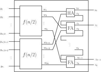
Figure 2: Recursive definition of an adder network.

Example 5.

Consider the constraint $y_{1}+y_{2}+y_{3}+y_{4}+y_{5}\leqslant 2$. The adder encoding introduces variables $w_{1},w_{2},w_{3},w_{4},c_{2},z_{0},z_{1},z_{2}$ defined as:

$$\begin{array}[]{lll}(w_{1},w_{2})=\operatorname{FA}(y_{1},y_{2},y_{3})&&(z_{0},c_{2})=\operatorname{HA}(w_{1},w_{3})\\ (w_{3},w_{4})=\operatorname{HA}(y_{4},y_{5})&&(z_{1},z_{2})=\operatorname{FA}(c_{2},w_{2},w_{4})\\ \end{array}$$

In addition, it enforces that $z_{0}+2z_{1}+4z_{2}\leqslant 2$, so it produces clauses $\{\neg z_{2},\neg z_{0}\vee\neg z_{1}\}$.

All in all, the encoding consists of the following clauses:

$$\begin{array}[]{lllll}\neg y_{1}\vee\neg y_{2}\vee\neg y_{3}\vee w_{1},&&\neg y_{1}\vee\neg y_{2}\vee y_{3}\vee\neg w_{1},&&\neg y_{1}\vee y_{2}\vee\neg y_{3}\vee\neg w_{1},\\ \neg y_{1}\vee y_{2}\vee y_{3}\vee w_{1},&&y_{1}\vee\neg y_{2}\vee\neg y_{3}\vee\neg w_{1},&&y_{1}\vee\neg y_{2}\vee y_{3}\vee w_{1},\\ y_{1}\vee y_{2}\vee\neg y_{3}\vee w_{1},&&y_{1}\vee y_{2}\vee y_{3}\vee\neg w_{1}&&\neg y_{1}\vee\neg y_{2}\vee w_{2},\\ \neg y_{1}\vee\neg y_{3}\vee w_{2},&&\neg y_{2}\vee\neg y_{3}\vee w_{2},&&y_{1}\vee y_{2}\vee\neg w_{2},\\ y_{1}\vee y_{3}\vee\neg w_{2},&&y_{2}\vee y_{3}\vee\neg w_{2},&&\neg y_{4}\vee\neg y_{5}\vee\neg w_{3},\\ \neg y_{4}\vee y_{5}\vee w_{3},&&y_{4}\vee\neg y_{5}\vee w_{3},&&y_{4}\vee y_{5}\vee\neg w_{3},\\ \neg y_{4}\vee\neg y_{5}\vee w_{4},&&y_{4}\vee\neg w_{4},&&y_{5}\vee\neg w_{4},\\ \neg w_{1}\vee\neg w_{3}\vee\neg z_{0},&&\neg w_{1}\vee w_{3}\vee z_{0},&&w_{1}\vee\neg w_{3}\vee z_{0},\\ w_{1}\vee w_{3}\vee\neg z_{0},&&\neg w_{1}\vee\neg w_{3}\vee c_{2},&&w_{1}\vee\neg c_{2},\\ w_{3}\vee\neg c_{2},&&\neg c_{2}\vee\neg w_{2}\vee\neg w_{4}\vee z_{1},&&\neg c_{2}\vee\neg w_{2}\vee w_{4}\vee\neg z_{1},\\ \neg c_{2}\vee w_{2}\vee\neg w_{4}\vee\neg z_{1},&&\neg c_{2}\vee w_{2}\vee w_{4}\vee z_{1},&&c_{2}\vee\neg w_{2}\vee\neg w_{4}\vee\neg z_{1},\\ c_{2}\vee\neg w_{2}\vee w_{4}\vee z_{1},&&c_{2}\vee w_{2}\vee\neg w_{4}\vee z_{1},&&c_{2}\vee w_{2}\vee w_{4}\vee\neg z_{1}\\ \neg c_{2}\vee\neg w_{2}\vee z_{2},&&\neg c_{2}\vee\neg w_{4}\vee z_{2},&&\neg c_{2}\vee\neg w_{4}\vee z_{2},\\ c_{2}\vee w_{2}\vee\neg z_{2},&&c_{2}\vee w_{4}\vee\neg z_{2},&&w_{2}\vee w_{4}\vee\neg z_{2},\\ \neg z_{2},&&\neg z_{0}\vee\neg z_{1}\\ \end{array}$$

Consider now the partial assignment $\{y_{1},y_{3},y_{4}\}$. Unit propagation just enforces $w_{2}$, but it does not detect any conflict. Therefore, the encoding is not consistent.

Theorem 6.

The adder encoding defined in this section encodes cardinality constraints with $O(n)$ variables and clauses. The encoding does not maintain consistency.

Proof.

The encoding does not maintain consistency due to the previous example. That the encoding needs $O(n)$ clauses and variables is shown by ? (?) in Lemma 2. ∎

3.2 Encoding Cardinality Constraints by Sorting the Input Variables

As before, let us consider the cardinality constraint $C:y_{1}+y_{2}+\cdots+y_{n}\leqslant a_{0}$. Let $s$ be the integer variable $s=y_{1}+y_{2}+\ldots+y_{n}$. The adder encoding introduced the Boolean variables $\operatorname{Logarithmic-Encoding}(s)$, and then easily encoded $s\leqslant a_{0}$. Here, the idea is introduce the Boolean variables $\operatorname{Order-Encoding}(s)$ and then encode $s\leqslant a_{0}$.

The way to introduce $\operatorname{Order-Encoding}(s)$ is by sorting the input variables: this is, given $y_{1},y_{2},\ldots,y_{n}$, we want to generate $z_{1},z_{2},\ldots,z_{n}$ such that $z_{1}\leqslant z_{2}\leqslant\cdots\leqslant z_{n}$ and $\{y_{1},y_{2},\ldots,y_{n}\}=\{z_{1},z_{2},\ldots,z_{n}\}$ as a multiset (i.e., there are the same number of true and false variables in both sides). There are different ways to construct encodings that perform such sorting. We present two ways, first totalizers and secondly odd-even sorters as an example for a comparator based sorting networks.

3.2.1 Sorting Variables with Totalizers

An encoding for cardinality constraints through totalizers was given by ? (?). The idea of the encoding is simple: given the input variables $y_{1},y_{2},\ldots,y_{n}$, the method splits the variables in two halves and recursively sorts both halves. Then, with a quadratic number of clauses, the method produces the sorted output. More specifically $(z_{1},z_{2},\ldots,z_{n})=\operatorname{Sort_{TOT}}(y_{1},y_{2},\ldots,y_{n})$ is defined by:

If $n=1$:

$z_{1}=y_{1}$.

If $n>1$:

Let us define

$$(w_{1},w_{2},\ldots,w_{n/2})=\operatorname{Sort_{TOT}}(y_{1},y_{2},\ldots,y_{n/2})$$

and

$$(w^{\prime}_{1},w^{\prime}_{2},\ldots,w^{\prime}_{n/2})=\operatorname{Sort_{TOT}}(y_{n/2+1},y_{n/2+2},\ldots,y_{n}).$$

Then:

$$z_{i}=\bigvee\{w_{j}\wedge w^{\prime}_{k}\ |\ j+k=i\},$$

where $w_{0}$ and $w^{\prime}_{0}$ are dummy true variables.

Example 7.

Let us consider again the constraint $y_{1}+y_{2}+y_{3}+y_{4}+y_{5}\leqslant 2$. The method of ? (?) introduces the following variables:

$$\begin{array}[]{lll}w_{1}=y_{1}\vee y_{2}&&w_{2}=y_{1}\wedge y_{2}\\ w_{3}=w_{1}\vee y_{3}&&w_{4}=y_{2}\vee(w_{1}\wedge y_{3})\\ w_{5}=w_{2}\wedge y_{3}&&w_{6}=y_{4}\vee y_{5}\\ w_{7}=y_{4}\wedge y_{5}&&z_{1}=w_{3}\vee w_{6}\\ z_{2}=w_{4}\vee(w_{3}\wedge w_{6})\vee w_{7}&&z_{3}=w_{5}\vee(w_{4}\wedge w_{6})\vee(w_{3}\wedge w_{7})\\ z_{4}=(w_{5}\wedge w_{6})\vee(w_{4}\wedge w_{7})&&z_{5}=w_{5}\wedge w_{7}\end{array}$$

Finally, the method adds the clause $\neg z_{3}$. All in all, the method produces the following set of clauses:

$$\begin{array}[]{lllll}\neg y_{1}\vee w_{1},&&\neg y_{2}\vee w_{1},&&y_{1}\vee y_{2}\vee\neg w_{1},\\ \neg y_{1}\vee\neg y_{2}\vee w_{2},&&y_{1}\vee\neg w_{2},&&y_{2}\vee\neg w_{2},\\ \neg w_{1}\vee w_{3},&&\neg y_{3}\vee w_{3},&&w_{1}\vee y_{3}\vee\neg w_{3},\\ \neg y_{2}\vee w_{4},&&\neg w_{1}\vee\neg y_{3}\vee w_{4},&&y_{2}\vee w_{1}\vee\neg w_{4},\\ y_{2}\vee y_{3}\vee\neg w_{4},&&\neg w_{2}\vee\neg y_{3}\vee w_{5},&&w_{2}\vee\neg w_{5},\\ y_{3}\vee\neg w_{5},&&\neg y_{4}\vee w_{6},&&\neg y_{5}\vee w_{6},\\ y_{4}\vee y_{5}\vee\neg w_{6},&&\neg y_{4}\vee\neg y_{5}\vee w_{7},&&y_{4}\vee\neg w_{7},\\ y_{5}\vee\neg w_{7},&&\neg w_{3}\vee z_{1},&&\neg w_{6}\vee z_{1},\\ w_{3}\vee w_{6}\vee\neg z_{1},&&\neg w_{4}\vee z_{2},&&\neg w_{3}\vee\neg w_{6}\vee z_{2},\\ \neg w_{7}\vee z_{2},&&w_{4}\vee w_{3}\vee w_{7}\vee\neg z_{2},&&w_{4}\vee w_{6}\vee w_{7}\vee\neg z_{2},\\ \neg w_{5}\vee z_{3},&&\neg w_{4}\vee\neg w_{6}\vee z_{3},&&\neg w_{3}\vee\neg w_{7}\vee z_{3},\\ w_{5}\vee w_{4}\vee w_{3}\vee\neg z_{3},&&w_{5}\vee w_{4}\vee w_{7}\vee\neg z_{3},&&w_{5}\vee w_{6}\vee w_{3}\vee\neg z_{3},\\ w_{5}\vee w_{6}\vee w_{7}\vee\neg z_{3},&&\neg w_{5}\vee\neg w_{6}\vee z_{4},&&\neg w_{4}\vee\neg w_{7}\vee z_{4},\\ w_{5}\vee w_{4}\vee\neg z_{4},&&w_{5}\vee w_{7}\vee\neg z_{4},&&w_{6}\vee w_{4}\vee\neg z_{4},\\ w_{6}\vee w_{7}\vee\neg z_{4},&&\neg w_{5}\vee\neg w_{7}\vee z_{5},&&w_{5}\vee\neg z_{5},\\ w_{5}\vee\neg w_{7},&&\neg z_{3}\end{array}$$

and maintains domain consistency. For instance, given the partial assignment $\{y_{1},y_{3}\}$ unit propagation enforces that $\neg w_{5},\neg w_{2},\neg y_{2},w_{1},w_{3},w_{4},\neg w_{6},\neg w_{7},\neg y_{4},\neg y_{5}$.

Theorem 8 (?).

The totalizer encoding defined in this section encode cardinality constraints with $O(n\log n)$ variables and $O(n^{2})$ clauses. The encoding maintains domain consistency.

3.2.2 Sorting Variables with Sorting Networks

An improved version of the previous encoding was given by  ? (?) by using a odd-even sorting network. To sort $n$ Boolean variables Odd-Even Sorting networks split the variables in two halves and recursively sort them. The merge of these two already sorted sets of variables is also done recursively. This is, $(z_{1},z_{2},\ldots,z_{n})=\operatorname{Sort_{OE}}(y_{1},y_{2},\ldots,y_{n})$ is defined by

If $n=1$:

$z_{1}=y_{1}$.

If $n>1$:

Let us define

$$(w_{1},w_{2},\ldots,w_{n/2})=\operatorname{Sort_{OE}}(y_{1},y_{2},\ldots,y_{n/2})$$

and

$$(w^{\prime}_{1},w^{\prime}_{2},\ldots,w^{\prime}_{n/2})=\operatorname{Sort_{OE}}(y_{n/2+1},y_{n/2+2},\ldots,y_{n}).$$

Then:

$$(z_{1},z_{2},\ldots,z_{n})=\operatorname{Merge_{OE}}(w_{1},w_{2},\ldots,w_{n/2};w^{\prime}_{1},w^{\prime}_{2},\ldots,w^{\prime}_{n/2}),$$

where

$$(z_{1},z_{2},\dots,z_{2n})=\operatorname{Merge_{OE}}(y_{1},y_{2},\ldots,y_{n};y^{\prime}_{1},y^{\prime}_{2},\ldots,y^{\prime}_{n})$$

is recursively defined as

If $n=1$:

$(z_{1},z_{2})=(y_{1}\vee y^{\prime}_{1},y_{1}\wedge y^{\prime}_{1})$.

If $n>1$:

Let us define

$$(w_{1},w_{3},\ldots,w_{2n-1})=\operatorname{Merge_{OE}}(y_{1},y_{3},\ldots,y_{n-1};y^{\prime}_{1},y^{\prime}_{3},\ldots,y^{\prime}_{n-1})$$

and

$$(w_{2},w_{4},\ldots,w_{2n})=\operatorname{Merge_{OE}}(y_{2},y_{4},\ldots,y_{2n};y^{\prime}_{2},y^{\prime}_{4},\ldots,y^{\prime}_{2n}).$$

Then:

$$\begin{array}[]{rcl}z_{1}&=&w_{1},\\ (z_{2},z_{3})&=&\operatorname{Merge_{OE}}(w_{2},w_{3}),\\ &\ldots\\ (z_{2n-2},z_{2n-1})&=&\operatorname{Merge_{OE}}(w_{2n-2},w_{2n-1}),\\ z_{2n}&=&w_{2n}.\end{array}$$

Figure 3 shows the recursive construction of sorting networks.

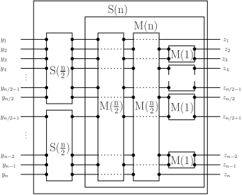
Figure 3: A sorting network and a merge of size $n$.

Theorem 9 (?).

The sorting network encoding defined in this section encodes cardinality constraints with $O(n\log^{2}n)$ variables and clauses. The encoding maintains domain consistency.

This method was improved first by ? (?) and then at by ? (?). In the first paper the authors reduce the size of the network by computing only the $a_{0}+1$ most significant bits. In this case, the encoding needs $O(n\log^{2}a_{0})$ variables and clauses without losing any propagation strength. Sorting Networks with fewer outputs than inputs are called cardinality Networks (which we denote by $\operatorname{CardinalityNetwork}$), and merge networks with fewer outputs than inputs are called simplified Merges (which we denote by $\operatorname{SimplifiedMerge}$).

The authors also change the base case of the definition of Merge from $z_{1}=y_{1}\vee y_{1}^{\prime}$ and $z_{2}=y_{1}\wedge y_{1}^{\prime}$ to $y_{1}\vee y_{1}^{\prime}\rightarrow z_{1}$ and $y_{1}\wedge y_{1}^{\prime}\rightarrow z_{2}$, halving the number of clauses needed. Note that this means that the outputs $z_{1},z_{2}$ are no longer functionally defined by the inputs $y_{1},y_{1}^{\prime}$.

In the second paper, the authors combine the recursive definitions of Sorting Network and Merge with naive ones (this is, without auxiliary variables). The naive encoding needs an exponential number of clauses, but it is more compact than the recursive one for small input sizes: therefore, the naive encoding can be used in some recursive calls. Using a dynamic programming approach, the authors achieve a much more compact encoding. The asymptotic size or propagation strength is the same that of ? (?), but in practice the encoding has better size and performance.

Example 10.

Let us consider again the constraint $y_{1}+y_{2}+y_{3}+y_{4}+y_{5}\leqslant 2$. The encoding of this section defines 10 variables

$$\begin{array}[]{rcl}(w_{1},w_{2},w_{3})&=&\operatorname{Order-Encoding}(y_{1}+y_{2}+y_{3})\\ (w_{4},w_{5})&=&\operatorname{Order-Encoding}(y_{4}+y_{5})\\ (z_{1},z_{2},z_{3},z_{4},z_{5})&=&\operatorname{Merge}(w_{1},w_{2},w_{3};w_{4},w_{5})\\ \end{array}$$

The encoding of ? (?) defines just 8 variables

$$\begin{array}[]{rcl}(w_{1},w_{2},w_{3})&=&\operatorname{CardinalityNetwork}(y_{1},y_{2},y_{3})\\ (w_{4},w_{5})&=&\operatorname{CardinalityNetwork}(y_{4},y_{5})\\ (z_{1},z_{2},z_{3})&=&\operatorname{SimplifiedMerge}(w_{1},w_{2},w_{3};w_{4},w_{5})\end{array}$$

and clauses

$$\begin{array}[]{lllll}\neg y_{1}\vee w_{1},&&\neg y_{2}\vee w_{1},&&\neg y_{3}\vee w_{1},\\ \neg y_{1}\vee\neg y_{2}\vee w_{2},&&\neg y_{1}\vee\neg y_{3}\vee w_{2},&&\neg y_{2}\vee\neg y_{3}\vee w_{2},\\ \neg y_{1}\vee\neg y_{2}\vee\neg y_{3}\vee w_{3},&&\neg y_{4}\vee w_{4},&&\neg y_{5}\vee w_{4},\\ \neg y_{4}\vee\neg y_{5}\vee w_{5},&&\neg w_{1}\vee z_{1},&&\neg w_{4}\vee z_{1},\\ \neg w_{2}\vee z_{2},&&\neg w_{1}\vee\neg w_{4}\vee z_{2},&&\neg w_{5}\vee z_{2},\\ \neg w_{3}\vee z_{3},&&\neg w_{2}\vee\neg w_{4}\vee z_{3},&&\neg w_{1}\vee\neg w_{5}\vee z_{3},\\ \neg z_{3}\\ \end{array}$$

The method is domain consistent: for instance, given the partial assignment $\{y_{1},y_{3}\}$ unit propagation enforces that $\neg z_{3},\neg w_{3},\neg y_{2},w_{1},w_{2},\neg w_{4},\neg w_{5},\neg y_{4},\neg y_{5}$.

A very similar encoding were given by ? (?) and ? (?). In this case the authors used a different definition of Sorting Networks, called Pairwise Sorting Networks by ? (?). By means of partial evaluation, this method also achieves $O(n\log^{2}a_{0})$ variables and clauses, and produce a similar encoding to those of ? (?) in terms of size and propagation strength.

4 Encoding Pseudo-Boolean Constraints into SAT

Pseudo-Boolean constraints are a well-studied topic in the SAT community. In this section we review the literature and provide a survey of the existing translations. PB constraints are a natural extension to cardinality constraints. As in the previous section, notice that the variables of these constraints are already propositional, so we do not have to encode them.

Let us fix the pseudo-Boolean constraint $a_{1}y_{1}+a_{2}y_{2}+\ldots+a_{n}y_{n}\leqslant a_{0}$. The direct translation without auxiliary variables generates one clause for each minimal subset of $\{y_{1}\ldots y_{n}\}$ such that the sum of the respective $a_{i}$ exceeds $a_{0}$. This translation is unique, but not practical since even simple PBs require $O(2^{n})$ clauses, as shown by  ? (?).

All the remaining methods in the literature introduce the integer variable $s=a_{1}y_{1}+a_{2}y_{2}+\ldots+a_{n}y_{n}$ and then simply encode $s\leqslant a_{0}$. The main differences between the encodings are the way to represent $s$ (either the order or the logarithmic encoding) and the way to enforce the definition of $s$.

We classify the encodings of PB constraints into three groups: the ones using binary adders to obtain the logarithmic encoding of $s$; the ones that use some sorting method to obtain the logarithmic encoding of $s$; and the ones that, incrementally, define the order encoding of the partial sums, obtaining finally the order encoding of $s$.

4.1 Encoding Pseudo-Boolean Constraints with Adders

Given positive integer numbers $a_{1},a_{2},\ldots,a_{n}$, an adder encoding for PB constraints defines propositional variables $z_{0},z_{1},\ldots,z_{m}$ such that

$$a_{1}y_{1}+a_{2}y_{2}+\ldots+a_{n}y_{n}=z_{0}+2z_{1}+2^{2}z_{2}+\ldots+2^{m}z_{m},$$

where $m=\left\lfloor\log(a_{1}+a_{2}+\ldots+a_{n})\right\rfloor$. In Section 3.1 we showed a method to accomplish this when $a_{1}=a_{2}=\cdots=a_{n}=1$. Here we extend this method for arbitrary positive coefficients.

First of all, for all $i$ in $\{1,2,\ldots,n\}$ let $(A_{i}^{0},A_{i}^{1},\ldots,A_{i}^{m})$ be the binary representation of $a_{i}$; this is, $A_{i}^{j}\in\{0,1\}$ and $a_{i}=A_{i}^{0}+2A_{i}^{1}+\cdots+2^{m}A_{i}^{m}$

Therefore, we obtain that

$$a_{1}y_{1}+a_{2}y_{2}+\ldots+a_{n}y_{n}=\\ =(A_{1}^{0}y_{1}+A_{2}^{0}y_{2}+\cdots+A_{n}^{0}y_{n})+\cdots+2^{m}(A_{1}^{m}y_{1}+\cdots+A_{n}^{m}y_{n}).$$

The goal of the encoding is to obtain the logarithmic encoding of that sum. This can be easily done by repeatedly using the Adder encoding for cardinality constraints explained in Section 3.1.

More specifically, let $z_{0}^{0},z_{0}^{1},\ldots,z_{0}^{m_{0}}$ be the logarithmic encoding of $A_{1}^{0}y_{1}+A_{2}^{0}y_{2}+\cdots+A_{n}^{0}y_{n}$, obtained as shown in Section 3.1. This means that

$$z_{0}^{0}+2z_{0}^{1}+\ldots+2^{m_{0}}z_{0}^{m_{0}}=A_{1}^{0}y_{1}+A_{2}^{0}y_{2}+\cdots+A_{n}^{0}y_{n}.$$

Let us define $z_{0}=z_{0}^{0}$. Therefore,

$$(A_{1}^{0}y_{1}+\cdots+A_{n}^{0}y_{n})+2(A_{1}^{1}y_{1}+\cdots+A_{n}^{1}y_{n})+2^{2}(A_{1}^{2}y_{1}+\cdots+A_{n}^{2}y_{n})+\cdots=\\ =z_{0}^{0}+2z_{0}^{1}+2^{2}z_{0}^{2}+\cdots+2(A_{1}^{1}y_{1}+\cdots+A_{n}^{1}y_{n})+2^{2}(A_{1}^{2}y_{1}+\cdots+A_{n}^{2}y_{n})+\cdots=\\ =z_{0}+2(A_{1}^{1}y_{1}+\cdots+A_{n}^{1}y_{n}+z_{0}^{1})+2^{2}(A_{1}^{2}y_{1}+\cdots+A_{n}^{2}y_{n}+z_{0}^{2})+\cdots$$

Again, let $z_{1}^{0},z_{1}^{1},\ldots,z_{1}^{m_{1}}$ be the logarithmic encoding of $A_{1}^{1}y_{1}+\cdots+A_{n}^{1}y_{n}+z_{0}^{1}$. Then, if we define $z_{1}=z_{1}^{0}$,

$$(A_{1}^{0}y_{1}+\cdots+A_{n}^{0}y_{n})+2(A_{1}^{1}y_{1}+\cdots+A_{n}^{1}y_{n})+2^{2}(A_{1}^{2}y_{1}+\cdots+A_{n}^{2}y_{n})+\cdots=\\ =z_{0}+2z_{1}+2^{2}(A_{1}^{2}y_{1}+\cdots+A_{n}^{2}y_{n}+z_{0}^{2}+z_{1}^{1})+\cdots$$

And so on and so forth until we obtain

$$(A_{1}^{0}y_{1}+A_{2}^{0}y_{2}+\cdots+A_{n}^{0}y_{n})+\cdots+2^{m}(A_{1}^{m}y_{1}+\cdots+A_{n}^{m}y_{n})=z_{0}+2z_{1}+\cdots+2^{m}z_{m}.$$

Example 11.

Let us consider the constraint $2y_{1}+3y_{2}+5y_{3}+6y_{4}\leqslant 9$. The Adder encoding first transforms the constraint into $y_{2}+y_{3}+2y_{1}+2y_{2}+2y_{4}+4y_{3}+4y_{4}\leqslant 9$. Then, using the circuit from Figure 4, defines the propositional variables $z_{0}^{0},z_{1}^{0},\ldots,z_{4}^{0}$. Finally, it enforces $z_{0}^{0}+2z_{1}^{0}+\cdots+16z_{4}^{0}\leqslant 9$ by adding clauses $\neg z_{4}^{0},\neg z_{3}^{0}\vee\neg z_{2}^{0},\neg z_{3}^{0}\vee\neg z_{1}^{0}$.

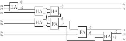
Figure 4: Adder circuit to encode $2y_{1}+3y_{2}+5y_{3}+6y_{4}\leqslant 9$.

The first encoding of PB constraints using some form of carry-adders was given by ? (?). ? (?) implemented a similar encoding in Minisat+, a PB extension to the award winning SAT solver Minisat.

Theorem 12 (Lemma 2 of ?).

The Adder encoding for PB presented in this section needs $O(\log(a_{0})n)$ variables and clauses, but does not maintain consistency.

4.2 Encoding Pseudo-Boolean Constraints with Sorting Methods

In this section we give the basic idea of encodings of Pseudo-Boolean constraints based on sorting methods (?, ?, ?). These encodings are extended to LI constraints in Section 5.4, so a more detailed explanation can be found there.

As in the previous section, given a PB constraint $a_{1}y_{1}+\ldots,+a_{n}y_{n}\leqslant a_{0}$, let $(A_{i}^{0},A_{i}^{1},\ldots,A_{i}^{m})$ be the binary representation of $a_{i}$. Then, the PB constraint can be written as

$$(A_{1}^{0}y_{1}+A_{2}^{0}y_{2}+\cdots+A_{n}^{0}y_{n})+\cdots+2^{m}(A_{1}^{m}y_{1}+\cdots+A_{n}^{m}y_{n})\leqslant a_{0}.$$

We can define Boolean variables

$$(z_{0}^{1},z_{0}^{2},\ldots,z_{0}^{k_{0}})=\operatorname{Sort}(A_{1}^{0}y_{1},A_{2}^{0}y_{2},\ldots,A_{n}^{0}y_{n}),$$

in a similar way as we did in Section 3.2. In this case, $z_{0}^{1}\leqslant z_{0}^{1}\leqslant\cdots\leqslant z_{0}^{k_{0}}$ and

$$A_{1}^{0}y_{1}+A_{2}^{0}y_{2}+\cdots+A_{n}^{0}y_{n}=z_{0}^{1}+z_{0}^{2}+\cdots+z_{0}^{k_{0}}.$$

Notice that given any $j>1$,

$$z_{0}^{j-1}\leqslant z_{0}^{j}\quad\Rightarrow\quad z_{0}^{j-1}+z_{0}^{j}=(\neg z_{0}^{j-1}\wedge z_{0}^{j})+2z_{0}^{j-1}.$$

So, if we define $w_{0}^{j}=\neg z_{0}^{j-1}\wedge z_{0}^{j}$,

$$A_{1}^{0}y_{1}+A_{2}^{0}y_{2}+\cdots+A_{n}^{0}y_{n}=z_{0}^{1}+z_{0}^{2}+\cdots+z_{0}^{k_{0}}=\\ =(w_{0}^{k_{0}}+w_{0}^{k_{0}-2}+\cdots)+2(z_{0}^{k_{0}-1}+z_{0}^{k_{0}-3}+\cdots)$$

Also notice that, by construction, $w_{0}^{k_{0}}+w_{0}^{k_{0}-2}+\cdots\leqslant 1$, so $w_{0}^{k_{0}}+w_{0}^{k_{0}-2}+\cdots=w_{0}^{k_{0}}\vee w_{0}^{k_{0}-2}\vee\cdots$ Let us define $z_{0}=w_{0}^{k_{0}}\vee w_{0}^{k_{0}-2}\vee\cdots$.

Then, we have that

$$a_{1}y_{1}+\ldots,+a_{n}y_{n}=(A_{1}^{0}y_{1}+\cdots+A_{n}^{0}y_{n})+2(A_{1}^{1}y_{1}+\cdots+A_{n}^{1}y_{n})+\cdots=\\ =z_{0}+2(A_{1}^{1}y_{1}+\cdots+A_{n}^{1}y_{n}+z_{0}^{k_{0}-1}+z_{0}^{k_{0}-3}+\cdots)+2^{2}(A_{1}^{2}y_{1}+\cdots$$

Repeating this process, we can define $z_{1},z_{2},\ldots,z_{l}$ so $a_{1}y_{1}+\cdots+a_{n}y_{n}=z_{0}+2z_{1}+\cdots+2^{l}z_{l}$. With these variables it is easy to enforce $z_{0}+2z_{1}+\cdots+2^{l}z_{l}\leqslant a_{0}$.

In summary, the method defines the variables:

$$\begin{array}[]{rcl}(z_{0}^{1},z_{0}^{2},\ldots,z_{0}^{k_{0}})&=&\operatorname{Sort}(A_{1}^{0}y_{1},A_{2}^{0}y_{2},\ldots,A_{n+1}^{0}y_{n+1})\\ (z_{1}^{1},z_{1}^{2},\ldots,z_{1}^{k_{1}})&=&\operatorname{Sort}(A_{1}^{1}y_{1},A_{2}^{1}y_{2},\ldots,A_{n+1}^{1}y_{n+1},z_{0}^{k_{0}-1},z_{0}^{k_{0}-3},\ldots)\\ &\cdots\\ (z_{l}^{1},z_{l}^{2},\ldots,z_{l}^{k_{l}})&=&\operatorname{Sort}(A_{1}^{l}y_{1},A_{2}^{l}y_{2},\ldots,A_{n+1}^{l}y_{n+1},z_{l-1}^{k_{l-1}-1},z_{l-1}^{k_{l-1}-3},\ldots)\\ \end{array}$$

$$w_{i}^{j}=\neg z_{i}^{j-1}\wedge z_{i}^{j}$$

$$z_{i}=w_{i}^{k_{i}}\vee w_{i}^{k_{i}-2}\vee\cdots$$

and then encodes $z_{0}+2z_{1}+\cdots+2^{l}z_{l}\leqslant a_{0}$.

Example 13.

Let us consider again the constraint $2y_{1}+3y_{2}+5y_{3}+6y_{4}\leqslant 9$. As before, the constraint is rewritten as $y_{2}+y_{3}+2y_{1}+2y_{2}+2y_{4}+4y_{3}+4y_{4}\leqslant 9$. Then, using the circuit from Figure 5, the encoding defines the propositional variables $z_{0},z_{1},\ldots,z_{4}$. Finally, it enforces $z_{0}+2z_{1}+\cdots+16z_{4}\leqslant 9$ by adding clauses $\neg z_{4},\neg z_{3}\vee\neg z_{2},\neg z_{3}\vee\neg z_{1}$.

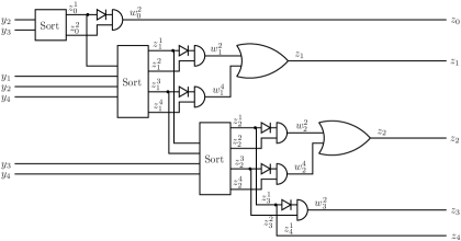
Figure 5: Circuit to encode $2y_{1}+3y_{2}+5y_{3}+6y_{4}\leqslant 9$ with sorting methods without tare.

An alternative method starts by introducing the so-called tare. This is, let $k$ be the minimal positive integer such that $2^{k}>a_{0}$. We can introduce a dummy true variable $y_{n+1}$ and encode the constraint $a_{1}y_{1}+\cdots+a_{n}y_{n}+(2^{k}-a_{0}-1)y_{n+1}\leqslant 2^{k}-1$. As before, we introduce the variables

$$\begin{array}[]{rcl}(z_{0}^{1},z_{0}^{2},\ldots,z_{0}^{l_{0}})&=&\operatorname{Sort}(A_{1}^{0}y_{1},A_{2}^{0}y_{2},\ldots,A_{n+1}^{0}y_{n+1})\\ (z_{1}^{1},z_{1}^{2},\ldots,z_{1}^{l_{1}})&=&\operatorname{Sort}(A_{1}^{1}y_{1},A_{2}^{1}y_{2},\ldots,A_{n+1}^{1}y_{n+1},z_{0}^{1},z_{0}^{3},\ldots)\\ \cdots\\ (z_{k}^{1},z_{k}^{2},\ldots,z_{k}^{l_{k}})&=&\operatorname{Sort}(A_{1}^{k}y_{1},A_{2}^{k}y_{2},\ldots,A_{n+1}^{k}y_{n+1},z_{k-1}^{1},z_{k-1}^{3},\ldots)\\ \end{array}$$

Now the original constraint can be enforced by simply adding the clause $\neg z_{k}$. Notice that in this case we do not have to introduce the variables $w_{i}^{j}$ and $z_{i}$, so the encoding is more compact. However, the encoding is not incremental: this is, if we encoded a PB constraint with bound $a_{0}$ and now we want to encode the same constraint with a new bound $a_{0}^{\prime}<a_{0}$, we have to re-encode the constraint from scratch. In the non-tare case, we would only need to enforce $z_{0}+2z_{1}+\cdots+2^{l}z_{l}\leqslant a_{0}^{\prime}$ for the new value $a_{0}^{\prime}$.

Example 14.

Again, let us consider the constraint $2y_{1}+3y_{2}+5y_{3}+6y_{4}\leqslant 9$. The tare is $15-9=6$, so we rewrite the constraint as $y_{2}+y_{3}+2y_{1}+2y_{2}+2y_{4}+2+4y_{3}+4y_{4}+4\leqslant 15$. Then, using the circuit from Figure 6, the encoding defines the propositional variable $z_{4}$. Now the constraint can be enforced by simply adding the clause $\neg z_{4}$.

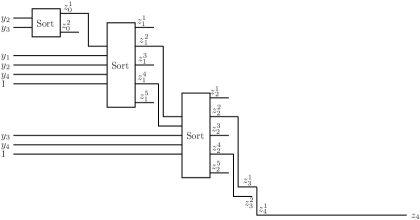
Figure 6: Circuit to encode $2y_{1}+3y_{2}+5y_{3}+6y_{4}\leqslant 9$ with sorting methods with tare.

? (?) designed and implemented this method in MiniSAT+. The coefficients are decomposed in a mixed radix form and Odd-Even sorting networks are used as the sorting method. They prove that their method maintains domain consistency on cardinality constraints, but it is not known what consistency is maintained in the pseudo-Boolean case. To our knowledge, this is still an open question. In Section 5.4 we answer this question: the encoding is consistent but not domain consistent. The method generates $O(N\log^{2}(N))$ variables and clauses, where $N=n\log(\max\{a_{i}\})$.

Another version of this encoding is presented by  ? (?). Their method, called global polynomial watchdog (GPW), adds the tare, decomposes the coefficients in binary and uses totalizers (see Section 3.2.1) as sorting method. The number of clauses of this encoding is $O(n^{2}\log(n)\log(a_{0}))$. It is proven that GPW detects inconsistencies and that through increasing the encoding by a factor of $n$, it also maintains domain consistency. The extended form is referred to as local polynomial watchdog (LPW).

? (?) improve the encoding of  ? (?) by using sorting networks instead of totalizers. Both constructions have the same consistency but Manthey’s save a factor of $n$ in size.

4.3 Encoding Pseudo-Boolean Constraints by Incremental Partial Sums

In this section we describe the encodings of PB constraints that introduce the order encoding of the partial sums.

The underlying idea of these encodings is simple. Given a PB constraint and $i\in\{0,1,\ldots,n\}$, let us define the integer variable $s_{i}=a_{1}y_{1}+\cdots+a_{i}y_{i}$. Since $s_{i}=s_{i-1}+a_{i}y_{i}$, where $s_{0}=0$, we can enforce the order encoding of these variables with the following clauses:

$$\begin{array}[]{ll}(s_{i-1}\geqslant j)\wedge y_{i}\rightarrow(s_{i}\geqslant j+a_{i}),&(s_{i-1}\geqslant j)\rightarrow(s_{i}\geqslant j,)\\ (s_{i-1}<j)\wedge\neg y_{i}\rightarrow(s_{i}<j),&(s_{i-1}<j)\rightarrow(s_{i}<j+a_{i}),\\ \end{array}$$ (1)

and then simply enforce $s_{n}\leqslant a_{0}$.

Notice, however, that the encoding contains some redundant variables. For instance, the variables $s_{1}\geqslant 1$, $s_{1}\geqslant 2$, $\ldots$ and $s_{1}\geqslant a_{1}$ are all equivalent. In fact, $s_{i}\geqslant j-1$ and $s_{i}\geqslant j$ are equivalent if there is no value of $y_{1},y_{2},\ldots,y_{i-1}$ with $a_{1}y_{1}+a_{2}y_{2}+\cdots+a_{i-1}y_{i-1}=j$. Therefore, we can just consider variables

$$\{s_{i}\geqslant j\ |\ \exists\ y_{1},y_{2},\ldots,y_{i-1}\in\{0,1\},\text{ with }a_{1}y_{1}+a_{2}y_{2}+\cdots+a_{i-1}y_{i-1}=j\}$$

and obtain an equivalent and more compact encoding.

The encoding of ? (?) computes all the possible values of the partial sums with diagrams like that shown in Figure 7.

Figure 7: A representation of partial sums calculated by the method of ? (?).

The method then adds a Boolean variable and the clauses of Equation (1) for each of these values. The encoding maintains domain consistency, but it is exponential in the worst case.

Notice that this diagram is a non-reduced BDD (see Section 5.3.1), and, therefore, the encoding of  ? (?) still contains redundant variables. The encoding is improved by ? (?), where the BDD is reduced before encoding it. The authors then encode the BDD with the Tseytin transformation by  ? (?), which requires one variable and six clauses per node. The method is domain consistent if the PB was sorted by the coefficients size.

Several improvements were made by ? (?). First, a faster algorithm for constructing the reduced BDD is presented. The authors can directly generate the reduced BDD, rather than constructing first the non-reduced one. The authors also introduce a CNF encoding for monotone BDDs that uses two clauses per BDD node and still maintains domain consistency via unit propagation. This encoding is more compact than the encodings used for general BDDs by previous work (?, ?) and shows improvement for practical SAT solving. The paper has also a deep analysis on the conditions under which the size of the BDD is polynomial in the number of literals.

Finally, the work by ? (?) generalizes the method of ? (?) for optimization functions: the authors study how to efficiently encode one PB constraint if the constraint with a different bound was already encoded.

Section 5.3 contains a detailed explanation of the generalization of PB encodings to LI constraints.

5 Encoding Linear Integer Constraints into SAT

In this section we study several translations of general LI constraints into CNF. One way to translate LI constraints is to encode the integer variables and uses PB translations from the previous Section. A different way extends the encodings from the previous section to integer variables. Following this path we introduce two new encodings, MDD in Section 5.3 and the family SN of encodings in Section 5.4.

Surprisingly, there are few publications that study the direct translations of non-pseudo-Boolean Linear Constraints to CNF.

In context of bounded model checking, ? (?) study the translation of LI constraints to BDDs via reformulating as PBs. We generalize and discuss this method in Section 5.6.

A different method by ? (?) using an order encoding of integers, and referred to as the Support encoding, is explained in detail in Section 5.5.

Many approaches to encoding linear constraints break the constraint into component, additions and multiplication by a constant. Hence $a_{1}x_{1}+\cdots+a_{n}x_{n}\leq a_{0}$ is encoded as $y_{i}=a_{i}x_{i},1\leq i\leq n$ and $y_{1}+\cdots+y_{n}\leq a_{0}$. Hence they effectively encode a summation constraint and multiplication by a constant. The systems below all follow this approach.

FznTini by  ? (?) uses a logarithmic encoding of signed integers. It uses ripple carry adders to encode summation, and shift and add to encode multiplication by a constant. FznTini uses an extra bit to check for overflow of arithmetic operations

BEE by ? (?) use an order encoding of integers. It encodes summation using odd-even sorting networks, and multiplication by a constant using repeated addition. BEE uses a equi-propagation to reason about relations amongst the Boolean variables created during encoding, and hence improve the encoding.

Picat SAT by ? (?) use a sign plus logarithmic encoding of magnitude to encode integers. Like Fzntini it uses ripple carry adders, and shift plus add to encode multiplication by a constant. Picat SAT applies equivalence optimization to remove duplicate Booleans that occur during the encoding procedure.

5.1 Encoding Linear Integer Constraints through the Order Encoding

In this section, we describe the encodings of LI constraints that use the order encoding.

Let $x$ be an integer variable with domain $[0,d]$, and let $\operatorname{Order-Encoding}(x)=[y^{1},y^{2},\ldots,y^{d}]$ be its order encoding. Notice that $x=y^{1}+y^{2}+\cdots+y^{d}$, since if $x=v$, then $y^{1}=y^{2}=\cdots=y^{v}=1$ and $y^{v+1}=y^{v+1}=\cdots=y^{d}=0$. Therefore, given a LI constraint $C:a_{1}x_{1}+\cdots+a_{n}x_{n}\leqslant a_{0}$, we can replace $C$ for the PB constraint

$$C^{\prime}:a_{1}(y_{1}^{1}+y_{1}^{2}+\cdots+y_{1}^{d_{1}})+\cdots+a_{n}(y_{n}^{1}+y_{n}^{2}+\cdots+y_{n}^{d_{n}})\leqslant a_{0}$$

If we now encode $C^{\prime}$ with a standard domain consistent PB encoding, the resulting encoding of $C$ will not be domain consistent. The reason for the loss of domain consistency can be seen in the next example:

Example 15.

Let us consider the constraint $C:x_{1}+x_{2}\leqslant 2$, where $x_{i}\in[0,2]$. Let $y_{i}^{1},y_{i}^{2}$ be the order encoding of $x_{i}$, and let us rewrite the constraint as $C^{\prime}:y_{1}^{1}+y_{1}^{2}+y_{2}^{1}+y_{2}^{2}\leqslant 2$.

Let us consider the naive encoding of $C^{\prime}$ with no auxiliary variables:

$$\begin{array}[]{l}\neg y_{1}^{1}\vee\neg y_{1}^{2}\vee\neg y_{2}^{1}\\ \neg y_{1}^{1}\vee\neg y_{1}^{2}\vee\neg y_{2}^{2}\\ \neg y_{1}^{1}\vee\neg y_{2}^{1}\vee\neg y_{2}^{2}\\ \neg y_{1}^{2}\vee\neg y_{2}^{1}\vee\neg y_{2}^{2}\\ \end{array}$$

This is obviously a domain consistent encoding of $C^{\prime}$: when two variables are set to true, unit propagation sets the other two to false. However, the resulting encoding is not a domain consistent encoding of $C$: if $y_{1}^{1}$ is set to true, unit propagation does not propagate anything; however, $y_{2}^{2}$ should be set to false (this is, if $x_{1}\geqslant 1$, then $x_{2}\leqslant 1$).

The reason is that we generated the encoding of $C^{\prime}$ without considering the relations on the variables of the constraint. Notice that, since $y_{i}^{j}$ are the order encoding of integer variables, they satisfy $y_{i}^{2}\rightarrow y_{i}^{1}$. If we use these clauses to simplify the previous encoding, we obtain:

$$\begin{array}[]{l}\neg y_{1}^{2}\vee\neg y_{2}^{1}\\ \neg y_{1}^{2}\vee\neg y_{2}^{2}\\ \neg y_{1}^{1}\vee\neg y_{2}^{2}\\ \end{array}$$

which is a domain consistent encoding of $C$.

This example shows that if we want to obtain an encoding with good properties, we have to consider the clauses from the order encoding of the integer variables. As we have seen in Section 4, there are basically two different approaches to domain consistent encodings of PB: using BDDs or using SNs. In this paper we adapt both of them to LI constraints: the BDD based approach is defined in Section 5.3, and the SN based approaches are defined in Section 5.4.

5.2 Preprocessing PB and LI constraints

Before describing the different approaches, there is an easy preprocessing step that reduces the encoding size without compromising the propagation strength:

Let us fix an LI constraint $C:a_{1}x_{1}+\cdots+a_{n}x_{n}\leqslant a_{0}$. Assume that some coefficients are equal; for simplicity, let us assume $a_{1}=a_{2}=\cdots=a_{r}$. In this case, we can define the integer variable $s=x_{1}+\cdots+x_{r}$ and decompose the constraint $C^{\prime}:a_{1}s+a_{r+1}x_{r+1}+\cdots+a_{n}x_{n}\leqslant a_{0}$ instead of $C$. The domain of $s$ is $[0,d_{s}]$ with $d_{s}=\min\{a_{0}/a_{1},d_{1}+\cdots+d_{r}\}$.

Notice that we do not need to encode the constraint $s=x_{1}+\cdots+x_{r}$ defining the integer variables $s$, instead we can encode $D\equiv s\geqslant x_{1}+\cdots+x_{r}$ since we are only interested in lower bounds. The encoding of $D$ can be done with sorting networks, which usually gives a more compact encoding than encoding $D$ as a LI constraint.

In our implementation we use the sorting networks defined by ? (?). However, any other methods based on computing the order encoding of $x_{1}+x_{2}+\ldots+x_{n}$, (e.g (?, ?)), could be used instead.

In industrial problems where constraints are not randomly generated, the coefficients have some meaning. Hence it is likely that a large LI constraint has only a few different coefficients. In this case this technique can be very effective.

Notice that this method can be used when $C$ is a pseudo-Boolean: however, $C^{\prime}$ is still a linear integer constraint. This technique can be used as a preprocessing method for pseudo-Boolean and linear constraints. After it, any method for encoding linear integer constraints, like the ones explained in the following sections, can be used.

5.3 Encoding Linear Integer Constraints through MDDs

In this section we will adapt the BDD construction of PB constraints of ? (?) to LI constraints, giving the encoding MDD. First, we develop the key notion for the MDD construction algorithm, the interval of a node. We then explain how to construct the MDD and present the encoding of MDDs in this context. Finally, we extend the method to optimization problems.

In the following, let us fix an LI constraint

$$C:a_{1}x_{1}+a_{2}x_{2}+\cdots+a_{n}x_{n}\leqslant a_{0}.$$

Let us define the Boolean variables $y_{i}^{j}$ such that

$$x_{i}=\operatorname{Order-Encoding}([y_{i}^{1},y_{i}^{2},\ldots,y_{i}^{d_{i}}]),\quad 1\leqslant i\leqslant n.$$

5.3.1 Multi-valued Decision Diagrams

A directed acyclic graph is called an ordered Multi-valued Decision Diagram if it satisfies the following properties:

• It has two terminal nodes, namely $\cal T$ (true) and $\cal F$ (false).

• Each non-terminal node is labeled by an integer variable $\{x_{1},x_{2},\cdots,x_{n}\}$. This variable is called selector variable.

• Every node labeled by $x_{i}$ has the same number of outgoing edges, namely $d_{i}+1$, each labeled by a distinct number in $\{0,1,\ldots,d_{i}\}$.

• If an edge connects a node with a selector variable $x_{i}$ and a node with a selector variable $x_{j}$, then $j>i$.

The MDD is quasi-reduced if no isomorphic subgraphs exist. It is reduced if, moreover, no nodes with only one child exist. A long edge is an edge connecting two nodes with selector variables $x_{i}$ and $x_{j}$ such that $j>i+1$. In the following we only consider quasi-reduced ordered MDDs without long edges, and we just refer to them as MDDs for simplicity.

An MDD represents a function

$$f:\{0,1,\ldots,d_{1}\}\times\{0,1,\ldots,d_{2}\}\times\cdots\times\{0,1,\ldots,d_{n}\}\rightarrow\{0,1\}$$

in the obvious way. Moreover, given the variable ordering, there is only one MDD representing that function. For further details about MDDs see e.g. ? (?).

An MDD where all the non-terminal nodes have exactly two edges is called Binary Decision Diagram or simply BDD. This is, BDDs are MDDs that non-terminal nodes are labeled by Boolean variables.

5.3.2 Motivation for using MDDs

As seen in Section 5.1, using the order encoding of integer variables, an LI constraint can be replaced by a PB constraint. This PB could be encoded as in  (?), but this is not a good idea since the resulting encoding does not consider the binary clauses of the order encoding. The next example shows that MDDs are the natural way to generalize BDDs:

Example 16.

Let us consider $n=2$, $a_{1}=1$, $d_{1}=3$, $a_{2}=2$, $d_{2}=2$ and $a_{0}=4$. Notice that $y_{1}^{1}+y_{1}^{2}+y_{1}^{3}=x_{1}$ and $y_{2}^{1}+y_{2}^{2}=x_{2}$. Therefore, we can rewrite the LI constraint as the pseudo-Boolean

$$C^{\prime}:y_{1}^{1}+y_{1}^{2}+y_{1}^{3}+2(y_{2}^{1}+y_{2}^{2})\leqslant 4.$$

The BDD of $C^{\prime}$ defined by ? (?) is shown in the upper leftmost diagram of Figure 8. Notice that some paths are incompatible with the binary clauses of the order encoding: for instance, $y_{1}^{1}=0,y_{1}^{2}=1$ is not possible. If we remove all the incompatible paths, we obtain the diagram shown at the upper rightmost diagram of Figure 8. This is, in fact, equivalent to the MDD of $C:x_{1}+2x_{2}\leqslant 4$ shown in the lowest diagram of Figure 8.

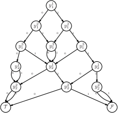
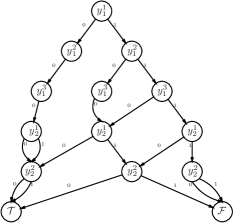
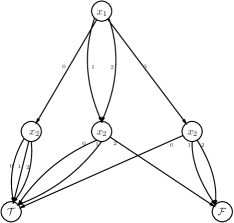
Figure 8: Decision Diagrams of $C^{\prime}:x_{1}+2x_{2}\leqslant 4$.

The previous example motivates the use of the MDD for LI constraints.

5.3.3 Interval of an MDD Node

In this section we define the interval of an MDD node. The definition is very similar to the BDD interval defined by ? (?); in fact, they coincide if the MDD is a BDD (i.e., $d_{i}=1$ for all $i$).

Let $\mathcal{M}$ be the MDD of $C$ and let $\nu$ be a node of $\mathcal{M}$ with selector variable $x_{i}$. We define the interval of $\nu$ as the set of values $\alpha$ such that the MDD rooted at $\nu$ represents the LI constraint $a_{i}x_{i}+\cdots+a_{n}x_{n}\leqslant\alpha$. It is easy to see that this definition corresponds in fact to an interval.

Example 17.

Figure 9 contains the MDD of $3x_{1}+2x_{2}+5x_{3}\leqslant 15$, where $x_{1}\in[0,4]$, $x_{2}\in[0,2]$ and $x_{3}\in[0,3]$. The root interval is $[15,15]$: this means that the root does not correspond to any constraint $3x_{1}+2x_{2}+5x_{3}\leqslant\alpha$, apart from $\alpha=15$. In particular, it means that this constraint is not equivalent to $3x_{1}+2x_{2}+5x_{3}\leqslant 14$ or $3x_{1}+2x_{2}+5x_{3}\leqslant 16$. However, the left node with selector variable $x_{2}$ has interval $[15,16]$. This means that $2x_{2}+5x_{3}\leqslant 15$ and $2x_{2}+5x_{3}\leqslant 16$ are both represented by the MDD rooted at that node. In particular, that means that $2x_{2}+5x_{3}\leqslant 15$ and $2x_{2}+5x_{3}\leqslant 16$ are two equivalent constraints.

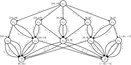
Figure 9: MDD of $3x_{1}+2x_{2}+5x_{3}\leqslant 15$.

The next proposition shows how to compute the intervals of every node:

Proposition 18.

Let $\mathcal{M}$ be the MDD of a LI constraint $a_{1}x_{1}+\cdots+a_{n}x_{n}\leqslant a_{0}$. Then, the following holds:

1. The interval of the true node ${\cal T}$ is $[0,\infty)$.

2. The interval of the false node ${\cal F}$ is $(-\infty,-1]$.

3. Let $\nu$ be a node with selector variable $x_{i}$ and children $\{\nu_{0},\nu_{1},\ldots,\nu_{d_{i}}\}$. Let $[\beta_{j},\gamma_{j}]$ be the interval of $\nu_{j}$. Then, the interval of $\nu$ is $[\beta,\gamma]$, with

   $$\beta=\max\{\beta_{r}+ra_{i}\ |\ 0\leqslant r\leqslant d_{i}\},\qquad\gamma=\min\{\gamma_{r}+ra_{i}\ |\ 0\leqslant r\leqslant d_{i}\}.$$

Example 19.

Again, let us consider the constraint $3x_{1}+2x_{2}+5x_{3}\leqslant 15$, whose MDD is represented at Figure 9. By the previous Proposition, ${\cal T}$ and ${\cal F}$ have, respectively, intervals $[0,\infty)$ and $(-\infty,-1]$. Applying again the same proposition, we can compute the intervals of the nodes having $x_{3}$ as selector variable. For instance, the interval from the left node is

$$[0,\infty)\cap[5,\infty)\cap[10,\infty)\cap[15,\infty)=[15,\infty),$$

and the interval from the node having selector variable $x_{3}$ in the middle is

$$[0,\infty)\cap[5,\infty)\cap(-\infty,9]\cap(-\infty,14]=[5,9].$$

After computing all the intervals from the nodes with selector variable $x_{3}$, we can compute the intervals of the nodes with selector variables $x_{2}$ in the same way, and, after that, we can compute the interval of the root.

5.3.4 Construction of the MDD

In this section we describe an efficient algorithm for building MDDs given an LI constraint $C$.

The key point of the MDDCreate algorithm, detailed in Algorithm 1 and Algorithm 2, is to label each node of the MDD with its interval $[\beta,\gamma]$.

In the following, for every $i\in\{1,2,\ldots,n+1\}$, we use a set $L_{i}$ consisting of pairs $([\beta,\gamma],\mathcal{M})$, where $\mathcal{M}$ is the MDD of the constraint $a_{i}x_{i}+\cdots+a_{n}x_{n}\leqslant a_{0}^{\prime}$ for every $a_{0}^{\prime}\in[\beta,\gamma]$ (i.e., $[\beta,\gamma]$ is the interval of $\mathcal{M}$). All these sets are kept in a tuple $\mathcal{L}=(L_{1},L_{2},\ldots,L_{n+1})$.

Note that by definition of the MDD’s intervals, if both $([\beta_{1},\gamma_{1}],\mathcal{M}_{1})$ and $([\beta_{2},\gamma_{2}],\mathcal{M}_{2})$ belong to $L_{i}$ then either $[\beta_{1},\gamma_{1}]=[\beta_{2},\gamma_{2}]$ or $[\beta_{1},\gamma_{1}]\cap[\beta_{2},\gamma_{2}]=\emptyset$. Moreover, the first case holds if and only if $\mathcal{M}_{1}=\mathcal{M}_{2}$. Therefore, $L_{i}$ can be represented with a binary search tree-like data structure, where insertions and searches can be done in logarithmic time. The function $\operatorname{\mathbf{search}}(K,L_{i})$ searches whether there exists a pair $([\beta,\gamma],\mathcal{M})\in L_{i}$ with $K\in[\beta,\gamma]$. Such a tuple is returned if it exists, otherwise an empty interval is returned in the first component of the pair. Similarly, we also use function $\operatorname{\mathbf{insert}}(([\beta,\gamma],\mathcal{M}),L_{i})$ for insertions. The size of the MDD in the worst case is $O(na_{0})$ (exponential in the size of the rhs coefficient) and algorithm complexity is $O(nw\log w)$ where $w$ is the maximum width of the MDD ($w\leq a_{0}$).

Algorithm 1 Procedure MDDCreate

0:  Constraint $C:a_{1}x_{1}+\cdots+a_{n}x_{n}\leqslant a_{0}$

0:  returns $\mathcal{M}$ the MDD of $C$.

1:  for all $i$ such that $1\leq i\leq n$ do

2:     $L_{i}\leftarrow\emptyset$.

3:  end for

4:  $L_{n+1}\leftarrow\Big{\{}\;\big{(}(-\infty,-1],{\cal F}\big{)},\;\;\big{(}[0,\infty),{\cal T}\big{)}\;\Big{\}}\Big{\}}$.

5:  $\mathcal{L}\leftarrow(L_{1},\ldots,L_{n+1})$.

6:  $([\beta,\gamma],\mathcal{M})\leftarrow\operatorname{\mathbf{MDDConstruction}}(1,a_{1}x_{1}+\cdots+a_{n}x_{n}\leqslant a_{0},\mathcal{L})$.

7:  return  $\mathcal{M}$.

Algorithm 2 Procedure MDDConstruction

0:  $i\in\{1,2,\ldots,n+1\}$, constraint $\tilde{C}:a_{i}x_{i}+\cdots+a_{n}x_{n}\leqslant a_{0}^{\prime}$ and tuple $\mathcal{L}$

0:  returns $[\beta,\gamma]$ interval of $\tilde{C}$ and $\mathcal{M}$ its MDD

1:  $([\beta,\gamma],\mathcal{M})\leftarrow\operatorname{\mathbf{search}}(a_{0}^{\prime},L_{i})$.

2:  if $[\beta,\gamma]\neq\emptyset$ then

3:     return  $([\beta,\gamma],\mathcal{M})$.

4:  else

5:     for all $j$ such that $0\leq j\leq d_{i}$ do

6:        $([\beta_{j},\gamma_{j}],\mathcal{M}_{j})\leftarrow\operatorname{\mathbf{MDDConstruction}}(i+1,a_{i+1}x_{i+1}+\cdots+a_{n}x_{n}\leqslant a_{0}^{\prime}-ja_{i},\mathcal{L})$.

7:     end for

8:     $\mathcal{M}\leftarrow$ mdd$(x_{i},[{\mathcal{M}}_{0},\ldots,{\mathcal{M}}_{d_{i}}])$.

9:     $[\beta,\gamma]\leftarrow[\beta_{0},\gamma_{0}]\cap[\beta_{1}+a_{1},\gamma_{1}+a_{1}]\cap\cdots\cap[\beta_{d_{i}}+d_{i}a_{i},\gamma_{d_{i}}+d_{i}a_{1}]$.

10:     $\operatorname{\mathbf{insert}}(([\beta,\gamma],\mathcal{M}),L_{i})$.

11:     return  $([\beta,\gamma],\mathcal{M})$.

12:  end if

The MDD creation works by initializing the $\mathcal{L}$ data structure for the terminal nodes ${\cal T}$ and ${\cal F}$, and the calling the MDD construction function. This checks if the MDD requires is already in the $\mathcal{L}$ structure in which case it is returned, otherwise if recursively builds the child MDDs for this node (adjusting the rhs of the constraint appropriately), and then constructs the MDD for this call using the function mdd to construct and nodes labelled by $x_{i}$ and the child MDDs. It calculates the interval for this MDD and returns the interval and MDD.

5.3.5 Encoding MDDs into CNF

In this section we generalize the encoding for monotonic BDDs described by ? (?) to monotonic MDDs. The encoding assumes that the selector variables are encoded with the order encoding.

Let $\mathcal{M}$ be an MDD with the variable ordering $[x_{1},\ldots,x_{n}]$. Let $[0,d_{i}]$ be the domain of the $i$-th variable, and let $\{y_{i}^{1},\ldots,y_{i}^{d_{i}}\}$ be the variables of the order encoding of $x_{i}$ (i.e., $y_{i}^{j}$ is true iff $x_{i}\geqslant j$). Let $\mu$ be the root of $\mathcal{M}$, and let ${\cal T}$ and ${\cal F}$ be respectively the true and false terminal nodes. In the following, given a non-terminal node $\nu$ of $\mathcal{M}$, we define $\operatorname{SelVar}(\nu)$ as the selector variable of $\nu$, and $\operatorname{Child}(\nu,j)$ as the $j$-th child of $\nu$, i.e., the child of $\nu$ defined by $\{\operatorname{SelVar}(\nu)=j\}$.

The encoding introduces the variables $\{z_{\nu}\ |\ \nu\in\mathcal{M}\}$; and the clauses

$$\{z_{\tau},\ \neg z_{{\cal F}}\}\cup\Big{\{}\ \neg z_{\nu}\lor\neg y_{i}^{j}\lor z_{\nu^{\prime}}\ |\ \nu\in{\mathcal{M}}\setminus\{{\cal T},{\cal F}\},\\ \operatorname{SelVar}(\nu)=x_{i},\ 0\leqslant j\leqslant d_{i},\ \nu^{\prime}=\operatorname{Child}(\nu,j)\Big{\}},$$

where $y_{i}^{0}$ is a dummy true variable ($x_{i}\geqslant 0$ since $x_{i}\in[0,d_{i}]$). This encoding will be denoted by $\operatorname{MDD-Enc}(\mu)$.

Notice that this encoding coincides with the BDD encoding of ? (?) if the MDD is a BDD.

Lemma 20.

Let $A=\{x_{j}\geqslant v_{j}\}_{j=i}^{n}$ be a partial assignment on the last variables. Let $\nu$ be a node of $\mathcal{M}$ with selector variable $x_{i}$.

Then, $\operatorname{MDD-Enc}(\mu)$ and $A$ propagates (by unit propagation) $\neg z_{\nu}$ if and only if $A$ is incompatible with $\nu$ (this is, the constraint defined by an MDD rooted at $\nu$ does not have any solution satisfying $A$).

Notice that the Lemma implies that $\operatorname{MDD-Enc}(\mu)$ is consistent.

Theorem 21.

Unit propagation on $\operatorname{MDD-Enc}(\mu)$ is domain consistent.

Proofs are in the Appendix.

Example 22.

Let us consider the MDD represented in Figure 9. The encoding introduces the variables $z_{1},z_{2},\ldots,z_{11},z_{{\cal T}},z_{{\cal F}}$, one for each node of the MDD; and the following clauses:

$${\begin{array}[]{l @{\hskip 15pt} l @{\hskip 15pt} l @{\hskip 15pt} l}z_{1},\hfil\hskip 15.0&z_{{\cal T}},\hfil\hskip 15.0&\neg z_{{\cal F}},\hfil\hskip 15.0&\neg z_{1}\lor z_{2},\\ \neg z_{1}\lor x_{1}\leqslant 0\lor z_{3},\hfil\hskip 15.0&\neg z_{1}\lor x_{1}\leqslant 1\lor z_{4},\hfil\hskip 15.0&\neg z_{1}\lor x_{1}\leqslant 2\lor z_{5},\hfil\hskip 15.0&\neg z_{1}\lor x_{1}\leqslant 3\lor z_{6},\\ \neg z_{2}\lor z_{7},\hfil\hskip 15.0&\neg z_{2}\lor x_{2}\leqslant 0\lor z_{8},\hfil\hskip 15.0&\neg z_{2}\lor x_{2}\leqslant 1\lor z_{8},\hfil\hskip 15.0&\neg z_{3}\lor z_{8},\\ \neg z_{3}\lor x_{2}\leqslant 0\lor z_{8},\hfil\hskip 15.0&\neg z_{3}\lor x_{2}\leqslant 1\lor z_{9},\hfil\hskip 15.0&\neg z_{4}\lor z_{9},\hfil\hskip 15.0&\neg z_{4}\lor x_{2}\leqslant 0\lor z_{9},\\ \neg z_{4}\lor x_{2}\leqslant 1\lor z_{9},\hfil\hskip 15.0&\neg z_{5}\lor z_{9},\hfil\hskip 15.0&\neg z_{5}\lor x_{2}\leqslant 0\lor z_{10},\hfil\hskip 15.0&\neg z_{5}\lor x_{2}\leqslant 1\lor z_{10},\\ \neg z_{6}\lor z_{10},\hfil\hskip 15.0&\neg z_{6}\lor x_{2}\leqslant 0\lor z_{10},\hfil\hskip 15.0&\neg z_{6}\lor x_{2}\leqslant 1\lor z_{11},\hfil\hskip 15.0&\neg z_{7}\lor z_{{\cal T}},\\ \neg z_{7}\lor x_{3}\leqslant 0\lor z_{{\cal T}},\hfil\hskip 15.0&\neg z_{7}\lor x_{3}\leqslant 1\lor z_{{\cal T}},\hfil\hskip 15.0&\neg z_{7}\lor x_{3}\leqslant 2\lor z_{{\cal T}},\hfil\hskip 15.0&\neg z_{8}\lor z_{{\cal T}},\\ \neg z_{8}\lor x_{3}\leqslant 0\lor z_{{\cal T}},\hfil\hskip 15.0&\neg z_{8}\lor x_{3}\leqslant 1\lor z_{{\cal T}},\hfil\hskip 15.0&\neg z_{8}\lor x_{3}\leqslant 2\lor z_{{\cal F}},\hfil\hskip 15.0&\neg z_{9}\lor z_{{\cal T}},\\ \neg z_{9}\lor x_{3}\leqslant 0\lor z_{{\cal T}},\hfil\hskip 15.0&\neg z_{9}\lor x_{3}\leqslant 1\lor z_{{\cal F}},\hfil\hskip 15.0&\neg z_{9}\lor x_{3}\leqslant 2\lor z_{{\cal F}},\hfil\hskip 15.0&\neg z_{10}\lor z_{{\cal T}},\\ \neg z_{10}\lor x_{3}\leqslant 0\lor z_{{\cal F}},\hfil\hskip 15.0&\neg z_{10}\lor x_{3}\leqslant 1\lor z_{{\cal F}},\hfil\hskip 15.0&\neg z_{10}\lor x_{3}\leqslant 2\lor z_{{\cal F}},\hfil\hskip 15.0&\neg z_{11}\lor z_{{\cal F}},\\ \neg z_{11}\lor x_{3}\leqslant 0\lor z_{{\cal F}},\hfil\hskip 15.0&\neg z_{11}\lor x_{3}\leqslant 1\lor z_{{\cal F}},\hfil\hskip 15.0&\neg z_{11}\lor x_{3}\leqslant 2\lor z_{{\cal F}}.\hfil\hskip 15.0\\ \end{array}}$$

In essence, for every node an auxiliary variable is introduced and for each edge a clause. Notice that some clauses are redundant. This issue is handled in the following Section.

Removing Subsumed Clauses

The MDD encoding explained here can easily be improved by removing some unnecessary clauses. We apply the following rule when producing the encoding:

Given a non-terminal node $\nu$ with $\operatorname{SelVar}(\nu)=x_{i}$, if $\operatorname{Child}(\nu,j)=\operatorname{Child}(\nu,j-1)$, then the clause $\neg z_{z}\nu\lor y_{i}^{j-1}\lor z_{\nu^{\prime}}$ is subsumed by the clause $\neg z_{\nu}\lor y_{i}^{j-2}\lor z_{\nu^{\prime}}$; therefore, we can remove it.

Additionally, we also improve the encoding by reinstating long edges (since the dummy nodes used to eliminate long edges do not provide any information); that is, we encode the reduced MDD instead of the quasi-reduced MDD.

Example 23.

Let us consider again the MDD represented in Figure 9. The encoding introduces the variables $z_{1},z_{2},z_{3},z_{5},z_{6},z_{8},z_{9},z_{10},z_{{\cal T}},z_{{\cal F}}$, one for each non-dummy node of the MDD; and the following clauses:

$${\begin{array}[]{l @{\hskip 15pt} l @{\hskip 15pt} l @{\hskip 15pt} l}z_{1},\hfil\hskip 15.0&z_{{\cal T}},\hfil\hskip 15.0&\neg z_{{\cal F}},\hfil\hskip 15.0&\neg z_{1}\lor z_{2},\\ \neg z_{1}\lor x_{1}\leqslant 0\lor z_{3},\hfil\hskip 15.0&\neg z_{1}\lor x_{1}\leqslant 1\lor z_{9},\hfil\hskip 15.0&\neg z_{1}\lor x_{1}\leqslant 2\lor z_{5},\hfil\hskip 15.0&\neg z_{1}\lor x_{1}\leqslant 3\lor z_{6},\\ \neg z_{2}\lor z_{{\cal T}},\hfil\hskip 15.0&\neg z_{2}\lor x_{2}\leqslant 0\lor z_{8},\hfil\hskip 15.0&\neg z_{3}\lor z_{8},\hfil\hskip 15.0&\neg z_{3}\lor x_{2}\leqslant 1\lor z_{9},\\ \neg z_{5}\lor z_{9},\hfil\hskip 15.0&\neg z_{5}\lor x_{2}\leqslant 0\lor z_{10},\hfil\hskip 15.0&\neg z_{6}\lor z_{10},\hfil\hskip 15.0&\neg z_{6}\lor x_{2}\leqslant 1\lor z_{{\cal F}},\\ \neg z_{8}\lor z_{{\cal T}},\hfil\hskip 15.0&\neg z_{8}\lor x_{3}\leqslant 2\lor z_{{\cal F}},\hfil\hskip 15.0&\neg z_{9}\lor z_{{\cal T}},\hfil\hskip 15.0&\neg z_{9}\lor x_{3}\leqslant 1\lor z_{{\cal F}},\\ \neg z_{10}\lor z_{{\cal T}},\hfil\hskip 15.0&\neg z_{10}\lor x_{3}\leqslant 0\lor z_{{\cal F}},\hfil\hskip 15.0\\ \end{array}}$$

5.3.6 Encoding Objective Functions with MDDs

In this section we describe how to deal with combinatorial problems where we minimize a linear integer objective function. A similar idea is used by ? (?), where the authors use BDDs for encoding problems with pseudo-Boolean objectives. Combinatorial optimization problems can be efficiently solved with a branch-and-bound strategy. In this way, all the lemmas learned in the previous steps are reused for finding the next solutions or proving the optimality. For implementing branch-and-bound, we need to be able to create a decomposition of the constraint $a_{1}x_{1}+\cdots+a_{n}x_{n}\leqslant a_{0}^{\prime}$ from the decomposition of $a_{1}x_{1}+\cdots+a_{n}x_{n}\leqslant a_{0}$ where $a^{\prime}_{0}<a_{0}$.

This is easy for cardinality constraints, since, when we have encoded a constraint $x_{1}+\cdots+x_{n}\leqslant a_{0}$ with a sorting network, we can encode $x_{1}+\cdots+x_{n}\leqslant a_{0}^{\prime}$ by adding a single clause see  (see ?).

Example 24.

Let us consider the easier case of a cardinality constraint objective. Assume we want to find a solution of a formula $F$ that minimizes the function $x_{1}+\cdots+x_{n}$, where $x_{i}$ are Boolean variables.

First, we launch a SAT solver with the input formula $F$. After finding a solution of cost $K$, the constraint $x_{1}+\cdots+x_{n}\leqslant K-1$ must be added. The encodings of cardinality constraints based on sorting networks introduce some variables $y_{1},\ldots,y_{K}$, where $y_{i}\equiv x_{1}+\cdots+x_{n}\geqslant i$. Let $S$ be such an encoding. We then launch the SAT solver with $F\cup S\cup\{\neg y_{K}\}$.

If now the SAT solver finds a solution of cost $K^{\prime}$, we just have to add the clause $\neg y_{K^{\prime}}$.

Example 24 shows that in optimization problems we do not have to re-encode the new constraints from scratch: we should reuse as much as the previous encodings as possible. In this way, not only do we generate fewer clauses and variables, but, more importantly, all the learned clauses about the previous encodings can be reused.

In order to reuse the previous encodings for the MDD encoding of an LI constraint, we have to save the tuple $\mathcal{L}$ used in Algorithm 1. When a new solution of cost $a^{\prime}_{0}+1$ is found, Algorithm 3 is called.

Algorithm 3 MDD Construction: Optimization version

0:  Constraint $C:a_{1}x_{1}+\cdots+a_{n}x_{n}\leqslant a^{\prime}_{0}$ and tuple $\mathcal{L}$.

0:  returns $\mathcal{M}$ the MDD of $C$.

1:  $([\beta,\gamma],\mathcal{M})\leftarrow\operatorname{\mathbf{MDDConstruction}}(1,a_{1}x_{1}+\cdots+a_{n}x_{n}\leqslant a^{\prime}_{0},\mathcal{L})$.

2:  return  $\mathcal{M}$.

Theorem 25.

Algorithm 3 provides a domain consistent encoding of the LI constraint $C$. The sum of all variables created by any call of Algorithm 3 is bound by $na_{0}$, and the number of clauses is bound by $na_{0}d$, where $d=\max\{d_{i}\}$ and $a_{0}$ is the cost of the first solution found.

Proof.

The encoding is domain consistent due to Theorem 21. Notice that the encoding creates at most one variable for every element of $L_{i}\in\mathcal{L}$, $1\leqslant i\leqslant n$. Therefore, after finding optimality, the encoding has generated at most $na_{0}$ variables in total. In the same way, the number of clauses generated can be bounded by $na_{0}d$. ∎

In practice the optimization version is very useful. The new MDD construction typically only adds a few nodes near the top of the MDD, and then reuses nodes below.

5.4 Encoding Linear Integer Constraints through Sorting Networks

In this section we introduce the methods SN-Tare and SN-Opt to encode LI constraints using Sorting Networks. We prove that they maintain consistency and discuss their size.

5.4.1 Background

The encodings in this section are a generalization of previous work encoding threshold functions to monotone circuits as in ? (?) and PB constraints to SAT (?, ?), that use different types of sorting networks to encode pseudo-Boolean constraints, explained in Section 4.2.

All these encodings work more or less in the same way: given a pseudo-Boolean constraint

$$a_{1}x_{1}+a_{2}x_{2}+\cdots+a_{n}x_{n}\leqslant a_{0}$$

and an integer number $b>1$, let $y_{0},y_{1},\ldots,y_{m}$ be the digits of $s=a_{1}x_{1}+a_{2}x_{2}+\cdots+a_{n}x_{n}$ in base $b$ (or, in fact, with a fixed mixed radix). The methods introduce the Boolean variables $y_{j}^{i}$ corresponding to the order encoding of $y_{j}$, and then encode $y_{0}+by_{1}+\cdots+b^{m}y_{m}\leqslant a_{0}$.

As we have seen in Section 4.2, there are two ways to encode PB constraints with sorting networks: either adding the tare or not.

When using a tare the methods add a dummy true variable $x_{n+1}$ with coefficient $a_{n+1}=b^{m+1}-a_{0}-1$ such that the bound in the constraint is $b^{m+1}-1$. In this case, the encoding is more compact, but it is not incremental. We generalize the tare case to LI constraints in Sections 5.4.2 and 5.4.3 and introduce encoding SN-Tare. The non-tare case, needed to encode objective functions, is studied in Section 5.4.5 and referred to as SN-Opt.

These methods are consistent but not domain consistent. Our implementation uses merge and simplified-merge networks (?), but any domain-consistent encoding of sorting networks can be used instead.

5.4.2 Encoding LI Constraints with Logarithmic Coefficients.

First, let us consider the simpler case where all the coefficients have a single digit in a fixed base $b>1$, and the bound is $a_{0}=b^{m+1}-1$ for some integer value $m$. In the next section we show that a general LI constraint can be reduced to this case.

Let us consider the constraint

$$\begin{array}[]{lccccccccc}C:&b^{0}\Big{(}A_{1,0}x_{1,0}&+&A_{2,0}x_{2,0}&+&\cdots&+&A_{n,0}x_{n,0}\Big{)}&+&\\ &b^{1}\Big{(}A_{1,1}x_{1,1}&+&A_{2,1}x_{2,1}&+&\cdots&+&A_{n,1}x_{n,1}\Big{)}&+&\\ &\lx@intercol\hfil\ldots\hfil\lx@intercol&+&\\ &b^{m}\Big{(}A_{1,m}x_{1,m}&+&A_{2,m}x_{2,m}&+&\cdots&+&A_{n,m}x_{n,m}\Big{)}&\leqslant&b^{m+1}-1,\end{array}$$

where the variables $x_{i,j}$ are integer with domain $[0,d_{i,j}]$ and $0\leqslant A_{i,j}<b.$

Given such a constraint, let us define

$$y_{j}=\begin{cases}A_{1,0}x_{1,0}+A_{2,0}x_{2,0}+\cdots+A_{n,0}x_{n,0}&\text{if }j=0\\ \left\lfloor{\frac{y_{j-1}}{b}}\right\rfloor+A_{1,j}x_{1,j}+A_{2,j}x_{2,j}+\cdots+A_{n,j}x_{n,j}&\text{if }j>0\\ \end{cases}$$

Proposition 26.

1. Given an integer $z$ with $\operatorname{Order-Encoding}(z)=[z^{1},z^{2},\ldots,z^{d}]$, then

   $$\operatorname{Order-Encoding}(\left\lfloor{\frac{z}{b}}\right\rfloor)=[z^{b},z^{2b},\ldots,z^{b\left\lfloor{\frac{d}{b}}\right\rfloor}]$$

   is a domain consistent encoding of $\left\lfloor{\frac{z}{b}}\right\rfloor$.

2. Given integers $z$ and $a$ with $\operatorname{Order-Encoding}(z)=[z^{1},z^{2},\ldots,z^{d}]$ and $a>0$,

   $$\operatorname{Order-Encoding}(az)=[\overbrace{z^{1},z^{1},\ldots,z^{1}}^{(a)},\overbrace{z^{2},z^{2},\ldots,z^{2}}^{(a)},\ldots,\overbrace{z^{d},z^{d},\ldots,z^{d}}^{(a)}]$$

   is a domain consistent encoding of $az$.

3. Given $n$ integer variables $z_{1},z_{2},\ldots,z_{n}$ with $\operatorname{Order-Encoding}(z_{i})=[z_{i}^{1},z_{i}^{2},\ldots,z_{i}^{d_{i}}]$,

   $$\operatorname{Order-Encoding}(z_{1}+z_{2}+\cdots+z_{n})=\\ =\operatorname{SortingNetwork}(z_{1}^{1},z_{1}^{2},\ldots,z_{1}^{d_{1}},z_{2}^{1},z_{2}^{2},\ldots,z_{2}^{d_{2}},\ldots,z_{n}^{d_{n}})$$

   is a domain consistent encoding of $z_{1}+z_{2}+\cdots+z_{n}$.

The proof of this proposition is trivial using the definitions of order encoding and sorting networks.

Now, given $(i,j)\in[1,n]\times[0,m]$, let us define the tuple $X_{i,j}$ as

$$X_{i,j}=\left(\overbrace{x_{i,j}^{1},x_{i,j}^{1},\ldots,x_{i,j}^{1}}^{(A_{i,j})},\overbrace{x_{i,j}^{2},x_{i,j}^{2},\ldots,x_{i,j}^{2}}^{(A_{i,j})},\ldots,\overbrace{x_{i,j}^{d_{i,j}},x_{i,j}^{d_{i,j}},\ldots,x_{i,j}^{d_{i,j}}}^{(A_{i,j})}\right),$$

where $(x_{i,j}^{1},\ldots,x_{i,j}^{d_{i,j}})=\operatorname{Order-Encoding}(x_{i,j})$.

The encoding of this section introduces Boolean variables $y_{i}^{j}$ defined as

$$\begin{array}[]{l}(y_{0}^{1},y_{0}^{2},\ldots)=\operatorname{SortingNetwork}(X_{1,0},X_{2,0},\ldots,X_{n,0})\\ (y_{1}^{1},y_{1}^{2},\ldots)=\operatorname{SortingNetwork}(y_{0}^{b},y_{0}^{2b},\ldots,X_{1,1},X_{2,1},\ldots,X_{n,1})\\ \cdots\\ (y_{m}^{1},y_{m}^{2},\ldots)=\operatorname{SortingNetwork}(y_{m-1}^{b},y_{m-1}^{2b},\ldots,X_{1,m},X_{2,m},\ldots,X_{n,m})\\ \end{array}$$

Lemma 27.

Let $A=\{x_{i,j}\geqslant v_{i,j}\}_{1\leqslant i\leqslant n,0\leqslant j\leqslant m}$ be an assignment. Then,

$$\sum\limits_{j=0}^{m}b^{j}\Big{(}A_{1,j}v_{1,j}+A_{2,j}v_{2,j}+\cdots+A_{n,j}v_{n,j}\Big{)}>b^{m+1}-1$$

if and only if $y_{m}^{b}$ is propagated to true.

Finally, the encoding introduces the clause $\neg y_{m}^{b}$. By the previous lemma, the encoding is consistent.

Example 28.

Let us fix $b=3$, and consider the constraint

$$C:2x_{1,0}+2x_{2,0}+2x_{3,0}+3x_{1,1}+3x_{2,1}+9x_{1,2}\leqslant 26,$$

where $x_{1,0}\in[0,2]$, $x_{2,0}\in[0,3]$, $x_{3,0}\in[0,1]$, $x_{1,1}\in[0,4]$, $x_{2,1}\in[0,3]$ and $x_{1,2}\in[0,1]$. Notice that $A_{3,1}=A_{2,2}=A_{3,2}=0$. Let us denote $(x_{i,j}^{1},x_{i,j}^{2},\ldots,x_{i,j}^{d_{i,j}})=\operatorname{Order-Encoding}(x_{i,j})$ as usual.

The encoding of this section defines Boolean variables

$$\{y_{0}^{j}\ |\ 1\leqslant j\leqslant 12\}\cup\{y_{1}^{j}\ |\ 1\leqslant j\leqslant 11\}\cup\{y_{2}^{j}\ |\ 1\leqslant j\leqslant 4\}$$

as

$$(y_{0}^{1},y_{0}^{2},\ldots,y_{0}^{12})=\\ =\operatorname{SortingNetwork}(x_{1,0}^{1},x_{1,0}^{1},x_{1,0}^{2},x_{1,0}^{2},x_{2,0}^{1},x_{2,0}^{1},x_{2,0}^{2},x_{2,0}^{2},x_{2,0}^{3},x_{2,0}^{3},x_{3,0}^{1},x_{3,0}^{1}),$$

$$(y_{1}^{1},y_{1}^{2},\ldots,y_{1}^{11})=\operatorname{SortingNetwork}(y_{0}^{3},y_{0}^{6},y_{0}^{9},y_{0}^{12},x_{1,1}^{1},x_{1,1}^{2},x_{1,1}^{3},x_{1,1}^{4},x_{2,1}^{1},x_{2,1}^{2},x_{2,1}^{3}),$$

$$(y_{2}^{1},y_{2}^{2},y_{2}^{3},y_{2}^{4})=\operatorname{SortingNetwork}(y_{1}^{3},y_{1}^{6},y_{1}^{9},x_{1,2}^{1}),$$

and the clause $\neg y_{2}^{3}$.

Figure 10 shows the definition of these variables. Notice that, by Proposition 26, $(y_{i}^{1},y_{i}^{2},\ldots,)=\operatorname{Order-Encoding}(y_{i})$.

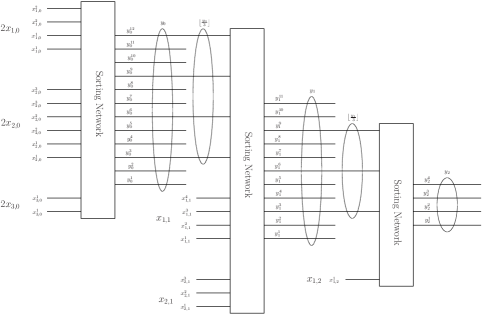
Figure 10: Network of the constraint $2x_{1,0}+2x_{2,0}+2x_{3,0}+3x_{1,1}+3x_{2,1}+9x_{1,2}\leqslant 26$.

The encoding maintains consistency: for instance, given the partial assignment

$$\{x_{1,0}=1,x_{2,0}\geqslant 1,x_{1,1}\geqslant 3,x_{2,1}=3,x_{3,1}=1\}$$

the first sorting network has 4 true inputs (two copies of $x_{1,0}^{1}$ and two copies of $x_{2,0}^{1}$): therefore, $y_{0}^{1},y_{0}^{2},y_{0}^{3}$ and $y_{0}^{4}$ are propagated to true (indeed, $y_{0}\geqslant 4$).

Now, the second sorting network has 7 true inputs: $y_{0}^{3},x_{1,1}^{1},x_{1,1}^{2},x_{1,1}^{3},x_{2,1}^{1},x_{2,1}^{2}$ and $x_{2,1}^{3}$. Therefore, $y_{1}^{j}$ is propagated to true for $1\leqslant j\leqslant 7$.

Finally, the last sorting network has 3 true inputs: $y_{1}^{3},y_{1}^{6}$ and $x_{1,2}^{1}$. Therefore, $y_{2}^{1}$, $y_{2}^{2}$ and $y_{2}^{3}$ are propagated. That conflicts with clause $\neg y_{2}^{3}$.

5.4.3 The SN-Tare Encoding for Linear Integer Constraints

In this section we transform a general LI constraint into a constraint where all the coefficients have a single digit in base $b$ and the bound is $b^{m+1}-1$. Then, the new constraint is encoded as in the previous section. We finally show that consistency is not lost.

Given a constraint $C:a_{1}x_{1}+\cdots+a_{n-1}x_{n-1}\leqslant a_{0}$, let $b$ be a fixed integer larger than 1. We define $m$ as the integer such that $b^{m}<a_{0}\leqslant b^{m+1}$, and $a_{n}=b^{m+1}-1-a_{0}$. Let $x_{n}$ be a dummy variable which is fixed to 1, i.e. $x_{n}=1$, called the tare. Then, the constraint is equivalent to

$$\begin{array}[]{lccccccccc}C^{\prime}:&b^{0}\Big{(}A_{1,0}x_{1}&+&A_{2,0}x_{2}&+&\cdots&+&A_{n,0}x_{n}\Big{)}&+&\\ &b^{1}\Big{(}A_{1,1}x_{1}&+&A_{2,1}x_{2}&+&\cdots&+&A_{n,1}x_{n}\Big{)}&+&\\ &\lx@intercol\hfil\ldots\hfil\lx@intercol&+&\\ &b^{m}\Big{(}A_{1,m}x_{1}&+&A_{2,m}x_{2}&+&\cdots&+&A_{n,m}x_{n}\Big{)}&\leqslant&b^{m+1}-1,\end{array}$$

where $(A_{i,0},A_{i,1},\ldots,A_{i,m})$ is the representation of $a_{i}$ in base $b$; this is,

$$a_{i}=\sum_{j=0}^{m}b^{j}A_{i,j},\text{ with }0\leqslant A_{i,j}<b.$$

Constraint $C^{\prime}$ can be encoded as in the previous section. We refer to this encoding as SN-Tare.

Example 29.

Consider the constraint $C:3x_{1}+2x_{2}+5x_{3}\leqslant 15$, where $x_{1}\in[0,4]$, $x_{2}\in[0,2]$ and $x_{3}\in[0,3]$. For base $b=3$, $m=2$ and the tare is $a_{4}=27-1-15=11$.

$C$ is therefore rewritten as $C^{\prime}:2x_{2}+2x_{3}+2x_{4}+3x_{1}+3x_{3}+9x_{4}\leqslant 26$.

SN-Tare introduces Boolean variables $y_{i}^{j}$ as shown in Figure 11. Then, it adds the clauses $\neg y_{2}^{3}\wedge x_{4}^{1}$.

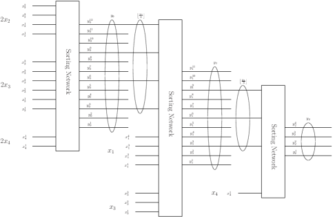
Figure 11: Network of the constraint $C:3x_{1}+2x_{2}+5x_{3}\leqslant 15$ with base $b=3$ using a tare as $x_{4}$.

The encoding is consistent. For example, if we take the assignment $\{x_{1}\geqslant 3,x_{3}\geqslant 2\}$, the first sorting network has 6 true input variables (two copies of $x_{3}^{1}$, two copies of $x_{3}^{2}$ and two copies of $x_{4}^{1}$). Therefore, $y_{0}^{j}$ will be propagated for $j\leqslant 6$.

Now, the second sorting network has 7 true input variables: $y_{0}^{3},y_{0}^{6},x_{1}^{1},x_{1}^{2},x_{1}^{3},x_{3}^{1}$ and $x_{3}^{2}$. Therefore, $y_{1}^{j}$ is propagated for $j\leqslant 7$.

Finally, the third network has 3 true inputs: $y_{1}^{3},y_{1}^{6}$ and $x_{4}^{1}$. This causes a conflict with clause $\neg y_{2}^{3}$.

However, the encoding is not domain consistent. If we take the assignment $\{x_{2}\geqslant 1\}$, the encoding propagates $x_{4}^{1},y_{0}^{1},y_{0}^{2},y_{0}^{3},y_{0}^{4},y_{1}^{1},y_{2}^{1},\neg y_{2}^{3}$. However, $\neg x_{3}^{3}$ is not propagated.

As shown in the previous example, domain consistency is lost due to the duplication of variables. The encoding, however, is consistent:

Theorem 30.

Let

$$C=C(x_{1,1},x_{1,2},\ldots,x_{1,m_{1}},x_{2,1},\ldots,x_{2,m_{2}},\ldots,x_{n,m_{n}})$$

be a monotonic constraint. Let

$$P=P(x_{1,1},x_{1,2},\ldots,x_{1,m_{1}},x_{2,1},\ldots,x_{2,m_{2}},\ldots,x_{n,m_{n}})$$

be a consistent propagator of $C$; i.e., given a partial assignment $A$ on the variables $\{x_{i,j}\}$, the propagator $P$ finds an inconsistency iff $A$ is inconsistent with $C$. Then,

$$P^{\prime}=P(x_{1},x_{1},\ldots,x_{1},x_{2},\ldots,x_{2},\ldots,x_{n})$$

is a consistent propagator of

$$C^{\prime}=C^{\prime}(x_{1},x_{2},\ldots,x_{n})=C(x_{1},x_{1},\ldots,x_{1},x_{2},\ldots,x_{2},\ldots,x_{n}).$$

Proof.

The key point in the proof is that, given the monotonicity of $C$, a partial assignment $\{x_{i,j}\geqslant v_{i,j}\}$ is inconsistent with $C$ if and only if $C(v_{1,1},\ldots,v_{n,m_{n}})$ is false.

Let $A=\{x_{i}\geqslant v_{i}\}_{i=1}^{n}$ be a partial assignment on the variables $x_{1},x_{2},\ldots,x_{n}$ inconsistent with $C^{\prime}$. That means that

$$C^{\prime}(v_{1},\ldots,v_{n})=C(v_{1},v_{1},\ldots,v_{1},v_{2},\ldots,v_{2},\ldots,v_{n})$$

is false. Therefore, $P(v_{1},v_{1},\ldots,v_{n})=P^{\prime}$ will find a conflict. ∎

Notice that the result does not extend to non-monotonic constraints:

Example 31.

Let us consider a constraint $C:x_{1}+x_{2}=1$, where $x_{i}$ are Boolean variables. Let $P$ be a propagator that, given a complete assignment of the variables, return a conflict if $C$ does not hold. Notice that $P$ is consistent. However, constraint $C^{\prime}:x+x=1$ is unsatisfiable. $P^{\prime}$ cannot find a conflict until $x$ is given a value and, therefore, is not a consistent propagator for $C^{\prime}$.

Also, notice that the result cannot be extended to domain consistency:

Example 32.

Consider the constraint $C:x_{1}+x_{2}\leqslant 1$, where $x_{i}$ are Boolean variables. Let $P$ be domain consistent encoding of $C$ created by the method of ? (?): it includes the auxiliary variable $y$ and the clauses

$$\neg x_{1}\vee y,\qquad\neg y\vee\neg x_{2}$$

Notice that $P$ is domain-consistent: if $x_{1}$ is assigned to true, the first clause propagates $y$ and the second one propagates $\neg x_{2}$. If $x_{2}$ is propagated to true, the second clause propagates $\neg y$ and the first one propagates $\neg x_{1}$.

If the constraint is replaced by $C^{\prime}:x+x\leqslant 1$, a domain consistent propagator would propagate $\neg x$. However, $P^{\prime}$ does not: clauses are $\{\neg x\vee y,\neg y\vee\neg x\}$, so unit propagation cannot propagate $\neg x$.

Theorem 33.

The encoding SN-Tare is consistent.

In SN-Tare variables are duplicated in the construction that consistency is shown for by Lemma 27. Thus by Theorem 30 consistency is maintained.

In the following Section we show an alternative proof that uses the fact that the underlying circuit only consist of AND and OR gates.

5.4.4 Monotone Circuits and Sorting Networks

The encoding SN-Tare is the CNF translation of a network of sorting networks. A sorting network is a network of comparators and a comparator computes the AND and OR of its inputs.

A circuit of AND and OR gates is called a monotone circuit. By introducing the tare in SN-Tare the underlying structure becomes a monotone circuit. The output variable of this circuit $y^{b}_{m}$ ( meaning $y_{m}\geq b$) is true if the partial assignment to the linear is greater than $b^{m+1}-1$, i.e. $\sum a_{i}x_{i}>b^{m+1}-1$, and otherwise undefined (see previous section).

We can take advantage of the fact that the circuit is monotone to show consistency of the translation to CNF. The key insight comes from the connection between CNF encodings of constraint propagators and monotone circuits as established by Bessiere et al in  (?). A partial assignment to the encoding of a monotone circuit can be interpreted as an assignment to the input of the circuit. Input variables to the circuit are set to true if they are true in the partial assignment, and false otherwise.

Using this connection, we show an alternative proof to Theorem 33, that is more compact than the proof in the previous Section or the similar result in context of PBs (?, ?) :

Theorem 33.

The encoding SN-Tare is consistent.

Proof.

By contradiction: Assume UP does not detect an inconsistency, i.e. assume a partial assignment $A$ such that the sum of the linear constraint exceeds $b^{m+1}-1$ and there is no conflict. The conflict can only occur between the unit clause $\neg y^{b}_{m}$ introduced by the encoding and a clause containing the literal $y^{b}_{m}$ that is propagated to true by UP under $A$ (see Lemma 27). Since there is no conflict, $y^{b}_{m}$ is unassigned and not forced to true by unit propagation . Consider now the total assignment $A^{\prime}$ which extends $A$ in a way that all unassigned variables are set to false, i.e. the remaining inputs of the circuit are set to false. The sum of the linear expression under $A^{\prime}$ and $A$ is the same.

It follows that all auxiliary variables introduced by the Tseytin encoding corresponding to output of gates that were unassigned, will also be forced to false by UP. There can be no inversion from false to true since the circuit does not contain negation. It follows that also the output gate of the circuit will be false. However, since all complete extensions of the partial assignment of $A$ must set the output gate of the circuit to true, there is a contradiction to the assumption. ∎

5.4.5 Encoding Objective Functions with Sorting Networks

The encoding of the previous section works for any LI constraint, but it is not incremental: this is, we cannot use the encoding of an LI constraint $C:\sum a_{i}x_{i}\leqslant a_{0}$ to construct the encoding of $C^{\prime}:\sum a_{i}x_{i}\leqslant a_{0}^{\prime}$. This is an issue in optimization problems, where a single constraint with different bounds is encoded.

In this section, we adapt our method to deal with optimization problems. As explained in Section 5.3.6, once we find a solution we do not want to encode the new constraint from scratch: we want to reuse the encoding of the previous constraint. As far as we know, this result is novel even for PB: there is no incremental encoding for pseudo-Booleans (or LI) through sorting networks.

The main difference between the encoding proposed here and the one for LI constraints described in the previous section is that here the tare cannot be used: the right hand side bound on the constraint is not a fixed value. Instead, we compute the value of the sum in the left side and compare it with the right side bound.

As in the previous sections, given a linear integer constraint

$$\sum_{i=0}^{n}a_{i}x_{i}\leqslant a_{0},$$

let us rewrite it as

$$\sum_{j=0}^{m}\sum_{i=1}^{n}b^{j}A_{ij}x_{i}\leqslant\sum_{j=0}^{m}b^{j}\varepsilon_{j},$$

where $b>1$ is the chosen base, $0\leqslant A_{ij}<b$, $0\leqslant\varepsilon_{j}<b$ and $m$ is large enough such that $\sum a_{i}d_{i}<b^{m+1}$ (i.e., the computed value $y_{m}<b$ for any input value of the variables $x_{i}$).

As in the previous sections, given $0\leqslant j\leqslant m$, we define

$$y_{j}=\begin{cases}\sum\limits_{i=1}^{n}A_{i,0}x_{i}&\text{if }j=0\\ \left\lfloor{\frac{y_{j-1}}{b}}\right\rfloor+\sum\limits_{i=1}^{n}A_{i,j}x_{i}&\text{if }j>0\\ \end{cases}$$

Variables $y_{j}$ are encoded as before with sorting networks; the input of these networks represents the order encoding of $y_{j}$. In the following, we denote

$$\operatorname{Order-Encoding}(y_{j})=[y_{j}^{1},y_{j}^{2},\ldots,y_{j}^{e_{j}}]$$

the output variables of these networks.

To encode the optimization function, besides these variables $y_{j}$, we also encode the following variables:

$$o_{j}^{k}:=\bigvee_{\begin{subarray}{c}1\leqslant l\leqslant e_{j}\\ l\equiv k\ (\text{mod }b)\end{subarray}}\Big{(}y_{j}^{l}\wedge\neg y_{j}^{l+b-k}\Big{)}\qquad 0\leqslant j\leqslant m,\ 1\leqslant k<b,$$ (2)

where $y_{j}^{l+b-k}$ is false if the domain of $y_{j}<l+b-k$. These variables $o_{j}^{k}$ can be easily defined through Tseytin transformation (?).

Finally, when we want to encode the constraint with a new bound $\sum\limits_{j=0}^{m}b^{j}\varepsilon_{j}$, the method just adds the following clauses:

$$\bigwedge_{\begin{subarray}{c}0\leqslant j_{1}\leqslant m\\ \varepsilon_{j_{1}}<b-1\end{subarray}}\Big{(}\neg o_{j_{1}}^{\varepsilon_{j_{1}}+1}\vee\bigvee_{\begin{subarray}{c}j_{1}<j_{2}\leqslant m\\ \varepsilon_{j_{2}}>0\end{subarray}}\neg o_{j_{2}}^{\varepsilon_{j_{2}}}\Big{)}$$ (3)

SN-Opt consists of the clauses encoding the sorting networks computing $y_{j}$ for $j=1\ldots m$, together with clauses (2) and (3).

Before proving that this encoding is consistent, we need the following result:

Lemma 34.

Given a partial assignment $A=\{x_{i}\geqslant v_{i}\}$ such that

$$\sum_{j=0}^{m}\sum_{i=1}^{n}b^{j}A_{ij}v_{i}=\sum_{j=0}^{m}b^{j}\varepsilon_{j},$$

the following variables are assigned due to unit propagation:

1. $o_{j}^{\varepsilon_{j}}$ for all $0\leqslant j\leqslant m$ with $\varepsilon_{j}>0$.

2. $\neg o_{j}^{\varepsilon_{j}+1}$ for all $0\leqslant j\leqslant m$ with $\varepsilon_{j}<b-1$.

3. $\neg x_{i}^{v_{i}+1}$ for all $1\leqslant i\leqslant n$ with some $A_{ij}\neq 0$ (i.e., $x_{i}\leqslant v_{i}$).

Theorem 35.

The encoding SN-Opt is consistent.

This Theorem answers an open question of ? (?) for the PB case, see appendix for the full proof of the general case for LI.

Example 36.

Consider again the constraint $C:3x_{1}+2x_{2}+5x_{3}\leqslant 15$, where $x_{1}\in[0,4]$, $x_{2}\in[0,2]$ and $x_{3}\in[0,3]$. Let us fix $b=3$. Since $\sum a_{i}d_{i}=31$, we can take $m=3$ ($31<b^{m+1}=81$).

The encoding introduces Boolean variables $y_{i}^{j}$ and $o_{i}^{j}$ as follows (see Figure 12):

$$\begin{array}[]{rcl}(y_{0}^{1},y_{0}^{2},\ldots,y_{0}^{10})&=&\operatorname{SortingNetwork}(x_{2}^{1},x_{2}^{1},x_{2}^{2},x_{2}^{2},x_{3}^{1},x_{3}^{1},x_{3}^{2},x_{3}^{2},x_{3}^{3},x_{3}^{3}),\\ (y_{1}^{1},y_{1}^{2},\ldots,y_{1}^{10})&=&\operatorname{SortingNetwork}(y_{0}^{3},y_{0}^{6},y_{0}^{9},x_{1}^{1},x_{1}^{2},x_{1}^{3},x_{1}^{4},x_{3}^{1},x_{3}^{2},x_{3}^{3}),\\ (y_{2}^{1},y_{2}^{2},y_{2}^{3})&=&\operatorname{SortingNetwork}(y_{1}^{3},y_{1}^{6},y_{1}^{9}),\\ y_{3}^{1}&=&y_{2}^{3}.\\ \end{array}$$

$$\begin{array}[]{rcl}o_{0}^{1}&=&(y_{0}^{1}\wedge\neg y_{0}^{3})\vee(y_{0}^{4}\wedge\neg y_{0}^{6})\vee(y_{0}^{7}\wedge\neg y_{0}^{9})\vee y_{0}^{10},\\ o_{0}^{2}&=&(y_{0}^{2}\wedge\neg y_{0}^{3})\vee(y_{0}^{5}\wedge\neg y_{0}^{6})\vee(y_{0}^{8}\wedge\neg y_{0}^{9}),\\ o_{1}^{1}&=&(y_{1}^{1}\wedge\neg y_{1}^{3})\vee(y_{1}^{4}\wedge\neg y_{1}^{6})\vee(y_{1}^{7}\wedge\neg y_{1}^{9})\vee y_{1}^{10},\\ o_{1}^{2}&=&(y_{1}^{2}\wedge\neg y_{1}^{3})\vee(y_{1}^{5}\wedge\neg y_{1}^{6})\vee(y_{1}^{8}\wedge\neg y_{1}^{9}),\\ o_{2}^{1}&=&y_{2}^{1}\wedge\neg y_{2}^{3},\\ o_{2}^{2}&=&y_{2}^{2}\wedge\neg y_{2}^{3}),\\ o_{3}^{1}&=&y_{3}^{1},\\ o_{3}^{2}&=&0.\\ \end{array}$$

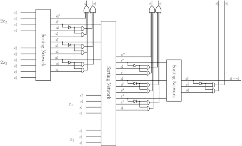
Figure 12: Network of the constraint $C:3x_{1}+2x_{2}+5x_{3}\leqslant 15$ with base $b=3$ without tare.

Since $15=0\cdot 3^{0}+2\cdot 3^{1}+1\cdot 3^{2}+0\cdot 3^{3}$, in this case $\varepsilon_{0}=0,\varepsilon_{1}=2,\varepsilon_{2}=1,\varepsilon_{3}=0$. Therefore, the method introduces the clauses

$$(\neg o_{0}^{1}\vee\neg o_{1}^{2}\vee\neg o_{2}^{1})\wedge\neg o_{2}^{2}\wedge\neg o_{3}^{1}$$

(see Equation (3)).

The encoding is consistent. For example, if we take the assignment $\{x_{1}\geqslant 3,x_{3}\geqslant 2\}$, the first sorting network has 4 true input variables (two copies of $x_{3}^{1}$ and two copies of $x_{3}^{2}$). Therefore, $y_{0}^{j}$ will be propagated for $j\leqslant 4$.

Now, the second sorting network has 6 true input variables: $y_{0}^{3},x_{1}^{1},x_{1}^{2},x_{1}^{3},x_{3}^{1}$ and $x_{3}^{2}$. Therefore, $y_{1}^{j}$ is propagated for $j\leqslant 6$.

Finally, the third network has 2 true inputs: $y_{1}^{3}$ and $y_{1}^{6}$: therefore, $y_{2}^{1}$ and $y_{2}^{2}$ are propagated.

By Equation (3), $\neg o_{3}^{1}$ is propagated: therefore, $y_{2}^{3}$ is set to false. Since $y_{2}^{2}$ is true, $o_{2}^{2}$ is propagated. That causes a conflict in Equation (3).

However, the encoding is not domain consistent. If we take the assignment $\{x_{2}\geqslant 1\}$, the encoding propagates $y_{0}^{1},y_{0}^{2},\neg o_{3}^{1},\neg o_{3}^{2},\neg o_{2}^{2},\neg y_{2}^{3}$ and $\neg y_{2}^{2}$. However, the encoding cannot propagate $\neg x_{3}^{3}$.

If now we wish to encode the constraint $C^{\prime}:3x_{1}+2x_{2}+5x_{3}\leqslant 10$ we only have to add the clauses

$$(\neg o_{0}^{2}\vee\neg o_{2}^{1})\wedge(\neg o_{1}^{1}\vee\neg o_{2}^{1})\wedge\neg o_{2}^{2}\wedge\neg o_{3}^{1}.$$

5.4.6 Practical Improvements and Size

In this section we describe improvements that can be applied to both SN-Tare and SN-Opt. We then prove the asymptotic size for both encodings using these improvements.

Notice that these encodings can use any domain consistent implementation of sorting networks; the concrete implementation or properties have not been used in any result. Our implementation uses the networks defined by ? (?), but this method can be replicated with any other implementation of sorting networks.

First of all, note that we do not have to encode all the bits of $y_{m}$: we only need the $b$ last bits. We can therefore replace the sorting networks by cardinality networks: when computing $y_{j}$, we need a $b^{m-j+1}$ cardinality network. For the lowest values of $j$, this value is larger than the input sizes of the network: in that case, the cardinality network is a usual sorting network. However, for the largest values of $j$, cardinality networks produce a more compact encoding.

Another important improvement is that we do not have to sort all the variables: some of them are already sorted. For instance , if we are computing $z_{1}+z_{2}$, then $z_{1}^{1}\leqslant z_{1}^{2}\leqslant\ldots\leqslant z_{1}^{d_{1}}$; and $z_{2}^{1}\leqslant z_{2}^{2}\leqslant\ldots\leqslant z_{2}^{d_{2}}$. Therefore, we can replace $\operatorname{CardinalityNetwork}(z_{1}^{1},z_{1}^{2},\ldots,z_{1}^{d_{1}},z_{2}^{1},z_{2}^{2},\ldots,z_{2}^{d_{2}})$ by $\operatorname{SimplifiedMerge}(z_{1},z_{2})$.

Also notice that if $x_{n}$ is the tare variable, $x_{n}=1$ by construction. Therefore, $\operatorname{SimplifiedMerge}(X;x_{n},\ldots,x_{n})=(X,x_{n},\ldots,x_{n})$: that is, we can remove the simplified merges involving the tare variable.

Furthermore, notice that the sum $y_{j}=\left\lfloor{\frac{y_{j-1}}{b}}\right\rfloor+A_{1,j}x_{1,j}+A_{2,j}x_{2,j}+\cdots+A_{n,j}x_{n,j}$ can be computed in several ways (using the associativity and commutativity properties of the sum). While the result is the same, the encoding size is not, since each way uses simplified merge networks of different sizes. (see Example 37). Finding the optimal order with respect to the size is hard; however, a greedy algorithm, where in each step we compute the sum of the two smallest terms, in practice gives good results.

Example 37.

Consider again constraint $C:3x_{1}+2x_{2}+5x_{3}\leqslant 15$, where $x_{1}\in[0,4]$, $x_{2}\in[0,2]$ and $x_{3}\in[0,3]$. Consider the tare case. Figures 13 and 14 contain the implementations of the method with different term orders in the computation of $y_{j}$. In Figure 13, we compute the values $y_{j}$ without reordering the terms, whereas in Figure 14 we reorder them to generate smaller networks.

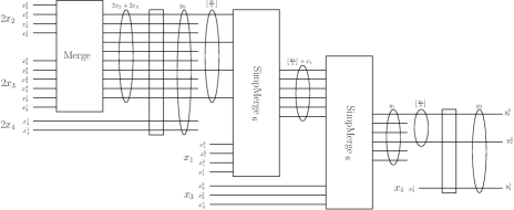
Figure 13: Network of the constraint $3x_{1}+2x_{2}+5x_{3}+11x_{4}\leqslant 26$, with $x_{4}=1$ without reordering the terms.

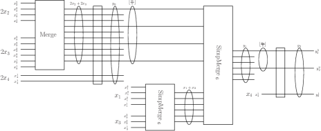
Figure 14: Network of the constraint $3x_{1}+2x_{2}+5x_{3}+11x_{4}\leqslant 26$, with $x_{4}=1$, after reordering the terms.

If we directly apply some method for encoding the sorting networks, some of the clauses would be subsumed by other ones. This happens because we have duplicated inputs in the network. The formula can be easily simplified once obtained. Alternatively, the use of $b=2$ produces simplified formulae directly.

Finally, we can omit redundant merge networks in the last layers. Let $a_{\max}=\max\{a_{i}~{}|~{}i\in 1..n\}$, the largest coefficient. We observe that the sorting networks after the $\log(a_{\max})$th level only merge already sorted output with the tare. Thus, they can be omitted. This effectively gives a better size. For instance, in Example 37 in both networks the last sorter is unnecessary as it merges the tare $x^{1}_{4}$ with an already sorted output. In fact, the output setting $\neg y^{3}_{2}$ is equivalent to $\neg y^{6}_{1}$. This discussion reduces the number of layers of sorters to $\log(a_{\max})$, which is fewer than $\log(a_{0})$.

Our implementation encodes each constraint with all the values of $b$ between 2 and 10, and it selects the most compact encoding. Almost always it is $b=2$, but the cost of trying other bases is negligible.

Theorem 38.

The encodings SN-Tare and SN-Opt using the improvements in this Section require $O(nd\log n\log d\log a_{\max})$ variables and clauses, where $d=\max\{d_{i}\}$.

5.5 Encoding Linear Integer Constraints through Partial Sums

In this section we explain the encoding of LI constraints of ? (?). Basically, the encoding introduces integer variables representing the partial sums $s_{i}=a_{i}x_{i}+a_{2}x_{2}+\cdots+a_{i}x_{i}$, which are encoded with the order encoding, and then simply encodes $s_{n}\leqslant a_{0}$. This encoding is called Support Encoding, since it encodes the support of the partial sums.

These partial sums can be easily encoded in a recursive way, this is, using that $s_{i}=s_{i-1}+a_{i}x_{i}$. Since, we are only interested in the positive polarity of $\operatorname{Order-Encoding}(s_{i})$ (only the lower bounds of the variables $x_{i}$ propagate), we can simply encode these equalities with the clauses

$$s_{i-1}\geqslant b\wedge x_{i}\geqslant c\rightarrow s_{i}\geqslant b+a_{i}c.$$

The encoding can be simplified as in  (?) since some of these clauses can be subsumed. All in all, the encoding needs $O(na_{0})$ variables and $O(nda_{0})$ clauses in the worst case, where $d$ is the size of the largest domain of the variables $x_{i}$.

The encoding is very similar to the MDD, MDD, encoding defined in Section 5.3. In fact, the clauses it introduces are identical to the MDD encoding from Section 5.3.5. Since this encoding does not check if two bounds of a partial sum are equivalent, the encoding is indeed equivalent to the MDD encoding when a non-reduced MDD is used.

In general, however, Support creates redundant clauses and variables which are not created using MDD. For instance, if $a_{i+1},a_{i+2},\ldots,a_{n}$ and $a_{0}$ are even, $s_{i}\geqslant 3$ and $s_{i}\geqslant 4$ are equivalent in the constraint. A reduced MDD will merge these two variables into a single node, while Support creates two different variables. In that aspect, our encoding MDD from Section 5.3 is an improved version of Support.

5.6 Encoding Linear Integer Constraints through the Logarithmic Encoding

In the previous sections we have seen some methods to handle LI constraints when integer variables are encoded with the order encoding. Here, we explain the different encodings when the logarithmic encoding is used. First, we explain the different possibilities described in the literature as well as some generalizations of PB encodings that work as well with LI constraints. Finally, we introduce a new method, BDD-Dec, more compact than most of the state-of-the-art encodings, but with a reasonable propagation strength.

Given a linear constraint

$$C:a_{1}x_{1}+a_{2}x_{2}+\cdots+a_{n}x_{n}\leqslant a_{0},$$

let $[y_{b,i}^{0},y_{b,i}^{1},\ldots,y_{b,i}^{\delta_{i}}]$ be $\operatorname{Logarithmic-Encoding}(x_{i})$ for $1\leqslant i\leqslant n$. In other words,

$$x_{i}=y_{b,i}^{0}+2y_{b,i}^{1}+\cdots+2^{\delta_{i}}y_{b,i}^{\delta_{i}},\text{ where }\delta_{i}=\log d_{i}\ \forall i\in\{1,2,\ldots,n\}.$$

5.6.1 Linear constraints as multiplication by a constant and summation

Perhaps the most obvious way to encode linear constraints is using a binary encoding of integers and using ripple carry adders to encode both addition and multiplication by a constant. This is the method used by both FznTini (?) and Picat SAT by  ? (?). Interestingly more complex adder circuits like carry look ahead adders, or parallel prefix adders, introduced by circuit designers to make addition circuits faster, appear to be worse for encoding arithmetic in SAT

In these methods the linear inequality $C$ is broken into $z_{i}=a_{i}x_{i},1\leq i\leq n$ and $z_{1}+\cdots+z_{n}\leq a_{0}$, and additions and multiplication by a constant are encoded using adder circuits.

A ripple carry adder encoding the addition of two non-negative $n$-bit logarithmic integers $u$ and $v$, $w=u+v$, where $\operatorname{Logarithmic-Encoding}(u)=[u_{b}^{0},u_{b}^{1},\ldots,u_{b}^{n-1}]$, $\operatorname{Logarithmic-Encoding}(v)=[v_{b}^{0},v_{b}^{1},\ldots,v_{b}^{n-1}]$ and $\operatorname{Logarithmic-Encoding}(w)=[w_{b}^{0},w_{b}^{1},\ldots,w_{b}^{n-1}]$ is simply

$$\begin{array}[]{rcl}(w_{b}^{0},c_{1})&=&HA(u_{b}^{0},v_{b}^{0})\\ (w_{b}^{1},c_{2})&=&FA(u_{b}^{1},v_{b}^{1},c_{1})\\ &\vdots\\ (w_{b}^{n-1},c_{n})&=&FA(u_{b}^{n-1},v_{b}^{n-1},c_{n-1})\\ \end{array}$$

where $c_{n}$ represents the overflow bit. It can be ignored (to implement fixed width arithmetic), or set to 0 (to force no overflow to occur). Repeated addition is achieved by recursively breaking the term $z_{1}+\cdots+z_{n}$ into two almost equal halves and summing the results of the addition of the halves.

Multiplication by a constant is implemented by binary addition of shifted inputs. Let $w=au$ where $a$ is a constant. The encoding is $w=\sum_{i=0..n-1,bit(i,a)=1}2^{i}u$ where $2^{i}u$ is calculated by right shifting the encoding for $u$ $i$ times, and the summation is encoded as above.

5.6.2 Linear constraints transformed to psuedo-Boolean constraints

In the remaning methods, the constraint is encoded in two steps: first, it is transformed into a PB constraint using logarithmic encodings of the integer variables. The PB constraint can subsequently be translated to CNF yielding a complete method, with one of the methods explained in Section 4.

Give the logarithmic encoding above the linear term is equivalent to

$$a_{1}x_{1}+a_{2}x_{2}+\cdots+a_{n}x_{n}=a_{1}(y_{b,1}^{0}+2y_{b,1}^{1}+\cdots+2^{\delta_{1}}y_{b,1}^{\delta_{1}})+\cdots+a_{n}(y_{b,n}^{0}+2y_{b,n}^{1}+\cdots+2^{\delta_{n}}y_{b,n}^{\delta_{n}}),$$

so $C$ is equivalent to

$$C^{\prime}:\sum_{i=0}^{n}\sum_{j=0}^{\delta_{i}}2^{j}a_{i}y_{b,i}^{j}\leqslant a_{0}.$$

Notice that $C^{\prime}$ is a pseudo-Boolean constraint, and it can be encoded with any pseudo-Boolean encoding. The size of $C^{\prime}$ is $O(n\log d)$, where $d=\max\{d_{i}\}.$ However, the method is not consistent, as it is shown in the following example:

Example 39.

Consider the constraint

$$C:4x_{1}+5x_{2}+6x_{3}\leqslant 14,\text{ where }x_{1},x_{2},x_{3}\in[0,2].$$

Using the method explained above, the constraint is transformed into

$$C^{\prime}:4y_{b,1}^{0}+8y_{b,1}^{1}+5y_{b,2}^{0}+10y_{b,2}^{1}+6y_{b,3}^{0}+12y_{b,3}^{1}\leqslant 14.$$

Notice that $C^{\prime}$ is equivalent to the following set of clauses

$$\begin{array}[]{lllllll}\{&\neg y_{b,1}^{0}\lor\neg y_{b,1}^{1}\lor\neg y_{b,2}^{0},&&\neg y_{b,1}^{0}\lor\neg y_{b,1}^{1}\lor\neg y_{b,3}^{0},&&\neg y_{b,1}^{0}\lor\neg y_{b,2}^{0}\lor\neg y_{b,2}^{1},\\ &\neg y_{b,1}^{0}\lor\neg y_{b,2}^{0}\lor\neg y_{b,3}^{0},&&\neg y_{b,1}^{0}\lor\neg y_{b,2}^{1}\lor\neg y_{b,3}^{0},&&\neg y_{b,1}^{0}\lor\neg y_{b,3}^{1},\\ &\neg y_{b,1}^{1}\lor\neg y_{b,2}^{1},&&\neg y_{b,1}^{1}\lor\neg y_{b,2}^{0}\lor\neg y_{b,3}^{0},&&\neg y_{b,1}^{1}\lor\neg y_{b,3}^{1},\\ &\neg y_{b,2}^{0}\lor\neg y_{b,2}^{1},&&\neg y_{b,2}^{0}\lor\neg y_{b,3}^{1},&&\neg y_{b,2}^{1}\lor\neg y_{b,3}^{0},\\ &\neg y_{b,2}^{1}\lor\neg y_{b,3}^{1},&&\neg y_{b,3}^{0}\lor\neg y_{b,3}^{1}&&&\}\end{array}$$

The constraint is unsatisfiable if $x_{1},x_{2},x_{3}\geqslant 1$. However, the logarithmic encoding of $x_{1},x_{2},x_{3}\geqslant 1$ is the empty assignment, so unit propagation cannot find any inconsistency.

The resulting PB constraint can be encoded with any method explained in Section 4. Let us consider the two main approaches for encoding PB constraints: SNs and BDDs.

Since the resulting method is not consistent, instead of an SN we can use adders: the propagation strength is similar but the resulting encoding is much smaller. The resulting encoding, Adder, is the most compact encoding, since it only needs $O(n\log d\log a_{\max})$ variables and clauses where $d=\max\{d_{i}\}$ and $a_{\max}=\max\{a_{i}~{}|~{}i\geq 1\}$, but it is also the worst encoding in terms of propagation strength.

Regarding the BDDs methods,  ? (?) realized that the BDD size of $C^{\prime}$ can be reduced by reordering the constraint. The resulting method, BDD, requires $O(na_{0}\log d)$.

In this paper we improved Bartzis and Bultan’s method by also decomposing the coefficients of $C^{\prime}$ before reordering. That generates a new encoding that we call BDD-Dec.

Example 40.

Consider the LI constraint $3x_{1}+2x_{2}+5x_{3}\leqslant 15$. After encoding the integer variables with the logarithmic encoding, the constraint becomes the pseudo-Boolean $3y_{b,1}^{0}+6y_{b,1}^{1}+12y_{b,1}^{2}+2y_{b,2}^{0}+4y_{b,2}^{1}+5x_{b,3}^{0}+10y_{b,3}^{1}\leqslant 15$. ? (?) construct the BDD of the pseudo-Boolean $2y_{b,2}^{0}+3y_{b,1}^{0}+4y_{b,2}^{1}+5y_{b,3}^{0}+6y_{b,1}^{1}+10y_{b,3}^{1}+12y_{b,1}^{2}\leqslant 15.$ Our method decomposes the coefficients (i.e., considers $y_{b,1}^{0}+2y_{b,1}^{0}$ instead of $3y_{b,1}^{0}$) and builds the resulting BDD; so we encode the constraint $y_{b,1}^{0}+y_{b,3}^{0}+2y_{b,2}^{0}+2y_{b,1}^{0}+2y_{b,1}^{1}+2y_{b,3}^{1}+4y_{b,2}^{1}+4y_{b,3}^{0}+4y_{b,1}^{1}+4y_{b,1}^{2}+8y_{b,3}^{1}+8y_{b,1}^{2}\leqslant 15.$

Formally, the BDD-Dec method encodes LI constraint $a_{1}x_{1}+\cdots+a_{n}x_{n}\leqslant a_{0}$ with $x_{i}\in[0,d_{i}],1\leq i\leq n$ by first creating the PB constraint

$$\sum_{i=1}^{n}\sum_{\begin{subarray}{c}0\leqslant j\leqslant\lfloor\log_{2}d_{i}\rfloor\\ (d_{i}\div 2^{j})\!\!\!\!\mod 2=1\end{subarray}}\sum_{\begin{subarray}{c}0\leqslant k\leqslant\lfloor\log_{2}a_{i}\rfloor\\ (a_{i}\div 2^{k})\!\!\!\!\mod 2=1\end{subarray}}2^{j+k}\times y_{b,i}^{j}\leqslant a_{0}$$

over the logarithmic encoding variables $y_{b}$ and encoding this using the state-of-the-art encoding for PB constraints given by ? (?).

Theorem 41.

Given a LI constraint $C:a_{1}x_{1}+a_{2}x_{2}+\cdots+a_{n}x_{n}\leqslant a_{0},$ BDD-Dec encodes $C$ with $O(n^{2}\log d\log a_{\max})$, where $a_{\max}$ is the largest coefficient and $d$ is the largest domain of the integer variables $x_{1},x_{2},\ldots,x_{n}$.

Notice that BDD-Dec encodes a PB with only power-of-two coefficients. Therefore, the theorem follows immediately from results of ? (?).

Notice that, since $n\log a_{\max}\ll a_{0}$, BDD-Dec is more compact than BDD.

6 Experimental Results

In this section we experimentally compare the main encodings of PB and LI constraints. We also want to check if our improvements work in practice: that is, if the preprocessing method explained in Section 5.2 improves some of the encodings, if MDD improves Support and if BDD-Dec improves BDD.

All experiments were performed in a 2x2GHz Intel Quad Core Xeon E5405, with 2x6MB of Cache and 16 GB of RAM. The Barcelogic SAT solver of ? (?) was used for all the SAT-based methods. We also compare against lazy clause generation (LCG)  (?) approaches which directly propagate linear constraints, and explain this propagation implemented in the Barcelogic SAT solver. We also compare against lazy decomposition (LD) (?, ?) methods, which use LCG propagation by default for all linear constraints, but during runtime decompose the most important linear constraints using some encoding, also implemented in the Barcelogic SAT solver.

Before commenting upon the results, let us explain the different families of benchmarks used. We use both PB benchmarks and general LI benchmarks.

6.1 Benchmarks

6.1.1 Pseudo-Boolean Benchmarks

RCPSP

Resource-constrained project scheduling problem (?) (RCPSP) is one of the most studied scheduling problem. It consists of tasks consuming one or more resources, precedences between some tasks, and resources. Here we consider the case of non-preemptive tasks and renewable resources with a constant resource capacity over the planning horizon. A solution is a schedule of all tasks so that all precedences and resource constraints are satisfied.

The objective of RCPSP is to find a solution minimizing the makespan. The problem is encoded the same way as by ? (?), resulting in one pseudo-Boolean constraints per resource and time slot. These PB constraints are then encoded with the different methods. Here we have considered the 2040 original RCPSP problems from PSPlib (?).

Pseudo-Boolean Competition 2015

Another set of problems we have considered is the benchmarks from the Pseudo-Boolean competition 2015 (http://pbeva.computational-logic.org/). We have considered the benchmarks from SMALL-INT optimization which contain Pseudo-Booleans (this is, we have removed benchmarks with only cardinality constraints or only clauses).

We have filtered some benchmarks that can be trivially solved by any method: from the 6266 benchmarks available, we have selected 3993 that cannot be solved by the PB solver Clasp (?) in 15 seconds. From these benchmarks, we have randomly selected 500.

Sport Leagues Scheduling

Another experiment considers scheduling a double round-robin sports league of $N$ teams. All teams meet each other once in the first $N-1$ weeks and again in the second $N-1$ weeks, with exactly one match per team each week. A given pair of teams must play at the home of one team in one half, and at the home of the other in the other half, and such matches must be spaced at least a certain minimal number of weeks apart. Additional constraints include, e.g., that no team ever plays at home (or away) three times in a row, other (public order, sportive, TV revenues) constraints, blocking given matches on given days, etc.

Additionally, the different teams can propose a set of constraints with some importance (low, medium or high). It is desired not only to maximize the number of these constraints satisfied, but also to assure that at least some of the constraints of every team are satisfied. More information can be found in the thesis of ? (?).

Low-importance constraints are given a weight of 1; medium-importance, 5, and high-importance, 10. For every constraint proposed by a team $i$, a new Boolean variable $x_{i,j}$ is created. This variable is set to true if the constraint is violated. For every team, a pseudo-Boolean constraint $\sum_{j}w_{i,j}x_{i,j}\leqslant K_{i}$ is imposed. The objective function to minimize is $\sum_{i}\sum_{j}w_{i,j}x_{i,j}$. The data is based on real-life instances.

We have considered 10 different problems with 20 random seeds. In all the problems, the optimal value was found around 30.

6.1.2 Linear Integer Benchmarks

Multiple Knapsack

Here we consider the classic multiple knapsack problem.

$$\begin{array}[]{lllllllllll}\text{Max }&a_{1}^{0}x_{1}&+&a_{2}^{0}x_{2}&+&\cdots&+&a_{n}^{0}x_{n}&&&\text{such that}\\ &a_{1}^{1}x_{1}&+&a_{2}^{1}x_{2}&+&\cdots&+&a_{n}^{1}x_{n}&\leqslant&a_{0}^{1}\\ &\ldots\\ &a_{1}^{m}x_{1}&+&a_{2}^{m}x_{2}&+&\cdots&+&a_{n}^{m}x_{n}&\leqslant&a_{0}^{m},\\ \end{array}$$

where $x_{i}$ are integer variables with domain $[0,d]$ and the coefficients belong to $[0,a_{\max}]$.

Since it only consists of linear integer constraints it is ideal for MIP solvers. We consider this problem since it is easy to modify the parameters of the constraints, and, therefore, we can easily compare the encodings in different situations. More precisely, we have considered different constraint sizes, coefficient sizes and domain sizes. In these problems, $n$ is the number of variables, $m=20$ is the number of LI constraints, $d+1$ is the domain size of the variables; and $a_{\max}$ is the bound of the coefficients.

For each parameter configuration, 100 benchmarks are considered. The experiments use $m=20$, $d=20$, $a_{\max}=10$ and $n=15$ unless stated otherwise.

Graph Coloring

The classical graph coloring problem consists in, given a graph, assign to each node a color $\{0,1,\ldots,c-1\}$ such that two nodes connected by an edge have different colors. Usually, the problem consists in finding a solution that minimizes the number of colors (i.e., $c$). Here we have considered a variant of this problem. Let us consider a graph that can be colored with $c$ colors: For each node $\nu$ of the graph, let us define an integer value $a_{\nu}$. Now, we want to color the graph with $c$ colors $\{0,1,\ldots,c-1\}$ minimizing the function $\sum a_{\nu}x_{\nu}$, where $x_{\nu}$ is the color of the node $\nu$.

We have considered the 80 graph coloring instances from http://mat.gsia.cmu.edu/COLOR08/ that have less than 500 nodes. For each graph problem, we have considered 4 different benchmarks: in the $i$-th one, $1\leqslant a_{\nu}\leqslant 3i-2$ for $i=1,2,3,4$.

MIPLib Benchmarks

Finally, we have considered the instances from MIPLib (?). These instances come from academia and industry.

Encoding methods perform well in problems with lots of Boolean variables and clauses and a small group of LI constraints; these problems mainly contain LI constraints, so we do not expect that our methods outperform MIP solvers. However, they are the standard tool to compare MIP solvers, and it is interesting to check how the different encodings perform in pure LI problems.

We have considered binary only problems and integer only problems with only integer coefficients and bounded domains. From them, we have selected the problems with domains ($d$) bounded by 100000, constraint size ($n$) bounded by 20000, coefficients ($a_{\max}$) bounded by 4000 and with less than 100000 constraints. We obtained 34 benchmarks, that have been run with 20 different random seeds.

6.2 Results Presentation

Multiple knapsack problems are very easy (Gurobi can solve any of them in less than one second), so results are reported using the average time for solving the instances. Timeouts are treated as a 300s response in computing average times.

In all the other problems we report the so-called pseudo-harmonic average distance from the solutions found and the best solutions known. Note that we do not use solving times but distances of solutions, and we do not compute the (arithmetic) average but the pseudo-harmonic one.

The usage of distances is motivated by the nature of the studied problems: they are much harder, most of the time they cannot be solved in 3600 seconds. Therefore, the solving time is not suitable: in most cases it would be 3600 seconds, and would give no information. For a method and a benchmark, we compute the distance from the best solution found by that method and the best solution known for the benchmark. If the method finds no solution, the distance is considered to be infinite. Notice that in this case we can compare two methods even if neither of them has found the optimal value.

Regarding the arithmetic mean, we do not use it for two reasons: first, since some distances are infinite, the mean will be infinite no matter the other values, making it impossible to compare methods. Second, the mean is highly affected for outliers, and we don’t wish the results to be so sensitive to them. For example, if we have 10 benchmarks and method 1 finds the optimal solution nine times and a solution at distance 1000 in the other one, and method 2 finds a solution at distance 100 in every case, both methods will have the same mean distance; but we want to conclude that method 1 is better than method 2.

The harmonic average solves these problems: it can be computed when some numbers are infinite, and it is more stable regarding outliers. However, the harmonic average cannot be computed if some value is 0. This is a problem in our case, since when a method finds the optimal solution, the distance of the solution found and the best solution is 0. For this reason, we have defined the pseudo-harmonic average as follows: given some non-negative numbers $x_{1},x_{2},\ldots,x_{n}$, let $H$ be the harmonic average of $x_{1}+1,x_{2}+1,\ldots,x_{n}+1$. Then, the pseudo-harmonic average of $x_{1},x_{2},\ldots,x_{n}$ is $H-1$.

More formally, the pseudo-harmonic average of $x_{1},x_{2},\ldots,x_{n}$ is

$$\frac{n}{\frac{1}{x_{1}+1}+\frac{1}{x_{2}+1}+\cdots+\frac{1}{x_{n}+1}}-1$$

When presenting some results, a value must be more than a $5\%$ better than another to be considered significantly better. If the difference of two values is less than $5\%$, we consider that there is no significant difference between them.

6.3 Grouping Variables with the Same Coefficient

In this section we test the impact of grouping variables with the same coefficient as a preprocessing technique in both Pseudo-Boolean and LI constraints, as explained in Section 5.2. This technique can be used with any consistent encoding or even with an LCG solver. Therefore, this technique is separately evaluated with the MDD encoding (MDD) explained in Section 5.3, the sorting network encoding (SN) explained in Section 5.4, with the support encoding (Support) from (?) explained in Section 5.5 and with an LCG approach (LCG).

Tables 2-7 contain the results of the different approaches. For each method, the best result is shown in bold (if it improves by more than 5%).

	15s	60s	300s	900s	3600s
MDD-Pre	0.616	0.462	0.284	0.201	0.16
MDD	0.639	0.541	0.351	0.253	0.189
SN-Pre	0.618	0.38	0.244	0.197	0.152
SN	0.692	0.439	0.263	0.228	0.18
Support-Pre	0.662	0.557	0.346	0.234	0.128
Support	0.674	0.544	0.326	0.244	0.173
LCG-Pre	0.655	0.535	0.325	0.21	0.118
LCG	0.335	0.166	0.117	0.124	0.13

Table 2: Grouping coefficients: pseudo-harmonic average distance from the 2040 original RCPSP benchmarks.

	15s	60s	300s	900s	3600s
MDD-Pre	27.2	15.8	9.12	6.86	4.67
MDD	17.6	10.1	6.13	4.45	3.08
SN-Pre	27.3	14.5	8.29	6.43	4.21
SN	23.7	9.75	6.3	4.48	3.36
Support-Pre	38.6	26.4	21.7	17.8	14.9
Support	38.2	30.4	21.9	15.8	13.9
LCG-Pre	19.4	8.37	4.99	3.88	2.91
LCG	15.1	7.24	4.96	3.90	3.00

Table 3: Grouping coefficients: pseudo-harmonic average distance from the 500 small-int PB optimization instances of the pseudo-Boolean competition 2015.

	15s	60s	300s	900s	3600s
MDD-Pre	917	331	38	7.84	5.56
MDD	1044	459	88.8	31.2	6.32
SN-Pre	27.9	12.1	2.5	1.28	0.748
SN	791	188	16.2	7.88	5.51
Support-Pre	951	364	33.6	8.21	5.88
Support	888	347	70.8	15.9	5.75
LCG-Pre	960	281	31.0	8.20	5.86
LCG	1517	342	47.4	13.0	7.51

Table 4: Grouping coefficients: pseudo-harmonic average distance from 200 sport scheduling league benchmarks.

	Different values of $n$						Different values of $a_{\max}$						Different values of $d$
	$5$	$10$	$20$	$40$	$80$	$160$	$1$	$2$	$4$	$8$	$16$	$32$	$1$	$2$	$4$	$10$	$25$	$100$
MDD-Pre	0.05	6.45	175	268	290	300	51.8	57.2	68.9	103	107	119	0.01	0.03	0.17	18.9	80.6	258
MDD	0.17	9.62	187	276	299	300	44.8	66.0	79.6	124	120	127	0.09	0.10	0.36	26.0	93.6	265
SN-Pre	0.24	10.4	181	267	289	300	56.0	65.5	67.6	122	118	122	0.14	0.23	0.47	20.3	93.8	261
SN	0.13	19.0	196	272	289	300	58.7	64.3	87.0	143	130	135	0.04	0.08	0.39	26.7	102	262
Support-Pre	0.24	17.2	196	277	300	300	108	99.4	98.3	142	134	147	0.05	0.17	0.60	30.7	110	279
Support	0.12	16.0	197	278	300	300	53.9	78.6	90.3	142	133	145	0.02	0.07	0.57	32.8	108	272
LCG-Pre	0.26	15.2	191	274	288	300	183	144	118	146	107	79.7	0.05	0.12	0.51	31.9	105	270
LCG	0.01	4.87	173	265	288	300	117	97.2	88.0	118	94.0	70.6	0.02	0.01	0.13	22.9	75.3	242

Table 5: Grouping coefficients: multiple knapsack average solving time.

	15s	60s	300s	900s	3600s
MDD-Pre	3.70	3.06	2.72	2.42	2.17
MDD	4.61	3.87	3.10	2.72	2.51
SN-Pre	3.50	2.99	2.64	2.45	2.45
SN	3.57	2.99	2.67	2.41	2.14
Support-Pre	3.24	2.45	2.06	1.82	1.54
Support	4.69	3.63	3.02	2.68	2.39
LCG-Pre	2.98	2.32	1.99	1.65	1.10
LCG	3.18	2.94	2.53	2.24	2.02

Table 6: Grouping coefficients: pseudo-harmonic average distance from 320 graph coloring benchmarks.

	15s	60s	300s	900s	3600s
MDD-Pre	3.43	2.47	1.76	1.31	0.767
MDD	2.40	2.03	1.42	1.15	0.981
SN-Pre	6.12	3.92	2.75	2.27	1.58
SN	6.32	4.30	2.71	2.42	1.82
Support-Pre	14.1	8.48	3.91	3.3	2.63
Support	6.69	3.54	2.42	1.72	1.12
LCG-Pre	11.5	5.49	3.33	1.98	1.62
LCG	1.85	1.39	1.19	1.01	0.90

Table 7: Grouping coefficients: pseudo-harmonic average distance from 680 MIPLib instances

Preprocessing clearly improves MDD results in Tables 2, 4, 5 and 6, and the basic method is better in Tables 3 and 7. It is worth noticing that SAT-based methods are not competitive method in Tables 3 and 7 (see Section 6.6), so MDD would not be the right choice anyway. Preprocessing helps MDD in all the cases where they are competitive, and, therefore, MDD should always be used with preprocessing. Accordingly, we will always use preprocessing on MDD in the following sections.

For SN, the basic method is only better than the method with preprocessing in Table 3; in the other cases, preprocessing is either better or both methods are roughly equal (Table 6). Again, it is worth noticing that for the problems of Table 3 SN is not a competitive choice. Preprocessing is helping SN in all the cases where encodings are competitive, and, therefore, SN should always be used with preprocessing. Accordingly, we will always use preprocessing on SN in the following sections.

Support-Pre is clearly better than Support in Table 6 and slightly better in Table 4, while the basic method is better in Tables 5 and 7. Again, the basic method is only better at cases where encodings should not be used: accordingly, we will always use preprocessing on Support in the following sections.

Preprocessing clearly improves LCG in Tables 4 and 6, and the basic method is better in the other cases. In this case, it is not clear if Preprocessing helps or not: accordingly, we will always use the method without preprocessing in the following sections.

6.4 BDDs with Logarithmic Encoding

As explained in Section 5.6, we can use the logarithmic encoding to transform an LI constraint into a PB. ? (?) realized that this PB can be reordered and then encoded into a BDD. This BDD can finally be encoded into SAT. We call BDD the resulting encoding. In Section 5.6 we propose an improvement of this method, called BDD-Dec, where the coefficients of the PB are also decomposed before producing the BDD: in this way, the BDD is smaller, so the resulting encoding generates fewer variables and clauses.

In this section we compare these two methods, to check if there is a significant improvement of our encoding BDD-Dec over BDD in practice.

Tables 8-10 contains the results of both methods in the different LI problems. Notice we have not compared these methods in the PB problems since they use the logarithmic encoding. In fact, the encoding BDD of a PB constraint would be equivalent to the encoding MDD.

	Different values of $n$						Different values of $a_{\max}$						Different values of $d$
	$5$	$10$	$20$	$40$	$80$	$160$	$1$	$2$	$4$	$8$	$16$	$32$	$1$	$2$	$4$	$10$	$25$	$100$
BDD	0.04	7.11	185	272	298	300	21.1	39.2	59.1	111	110	129	0.01	0.06	0.58	26.8	77.6	220
BDD-Dec	0.12	4.73	163	267	295	300	10.5	25.6	47.7	90.9	84.8	82.5	0.07	0.13	0.46	18.6	56.3	202

Table 8: BDDs methods: multiple knapsack average solving time.

	15s	60s	300s	900s	3600s
BDD	11.5	10.4	9.35	7.32	5.82
BDD-Dec	10.2	7.06	6.19	5.22	4.60

Table 9: BDDs methods: pseudo-harmonic average distance from 320 graph coloring benchmarks.

	15s	60s	300s	900s	3600s
BDD	6.59	4.53	2.89	2.49	2.20
BDD-Dec	9.88	8.86	5.77	4.78	3.56

Table 10: BDDs methods: pseudo-harmonic average distance from 680 MIPLib instances

BDD-Dec is clearly better at multiple knapsack and graph coloring, while BDD is the best choice for the MIPLib instances.

6.5 Domain consistent encodings for LI constraints.

In this section we compare the two domain consistent encodings for LI (and PB) constraints: Support, from ? (?) explained in Section 5.5, and our method MDD, explained in Section 5.3. As discussed in Section 5.5, both methods are basically equivalent except that Support generates a non-reduced MDD, and, therefore, produces redundant variables and clauses. We want to test here whether this redundancy makes MDD better than Support in practice.

Tables 11-16 contain the results of both methods in the different benchmarks. According to the results of the previous section, both methods use the preprocessing method described in Section 5.2.

	15s	60s	300s	900s	3600s
MDD	0.616	0.462	0.284	0.201	0.160
Support	0.662	0.557	0.346	0.234	0.128

Table 11: Domain consistent methods: pseudo-harmonic average distance from the 2040 original RCPSP benchmarks.

	15s	60s	300s	900s	3600s
MDD	27.2	15.8	9.12	6.86	4.67
Support	38.6	26.4	21.7	17.8	14.9

Table 12: Domain consistent methods: pseudo-harmonic average distance from the 500 small-int PB optimization instances of the pseudo-Boolean competition 2015.

	15s	60s	300s	900s	3600s
MDD	917	331	38	7.84	5.56
Support	951	364	33.6	8.21	5.88

Table 13: Domain consistent methods: pseudo-harmonic average distance from 200 sport scheduling league benchmarks.

	Different values of $n$						Different values of $a_{\max}$						Different values of $d$
	$5$	$10$	$20$	$40$	$80$	$160$	$1$	$2$	$4$	$8$	$16$	$32$	$1$	$2$	$4$	$10$	$25$	$100$
MDD	0.05	6.45	175	268	290	300	51.8	57.2	68.9	103	107	119	0.01	0.03	0.17	18.9	80.6	258
Support	0.12	16.0	197	278	300	300	53.9	78.6	90.3	142	133	145	0.02	0.07	0.57	32.8	108	272

Table 14: Domain consistent methods: multiple knapsack average solving time.

	15s	60s	300s	900s	3600s
MDD	3.70	3.06	2.72	2.42	2.17
Support	3.24	2.45	2.06	1.82	1.54

Table 15: Domain consistent methods: pseudo-harmonic average distance from 320 graph coloring benchmarks.

	15s	60s	300s	900s	3600s
MDD	3.43	2.47	1.76	1.31	0.767
Support	14.1	8.48	3.91	3.30	2.63

Table 16: Domain consistent methods: pseudo-harmonic average distance from 680 MIPLib instances

Support is better at graph coloring, but MDD is better at the other instances. The experimental results, then, prove that MDD improves Support. Accordingly, we will use MDD as the domain consistent encoding for LI constraints in the following experiments.

6.6 Comparison against Other Methods

In this section we compare the best encodings with other methods for solving MIP problems. The encodings selected are Adder, explained in Sections 4.1 and 5.6; BDD-Dec, explained in Section 5.6; SN, explained in Section 5.4; and MDD, explained in Section 5.3.

Other methods considered here are the LCG solver Barcelogic (?) for LI constraints (LCG); a lazy decomposition solver based on the SN encoding, LD-SN; a lazy decomposition solver based on the MDD encoding, LD-MDD; and the MIP solver Gurobi (?).

Methods MDD, SN, LD-SN and LD-MDD include the preprocessing technique described in Section 5.2. Results are given in Tables 17-22. For each family of benchmarks, the best encoding is underlined and the best method is shown in bold.

	15s	60s	300s	900s	3600s
Adder	16.7	11.1	2.99	2.37	1.43
SN	0.618	0.380	0.244	0.197	0.152
MDD	0.616	0.462	0.284	0.201	0.160
LD-SN	0.343	0.176	0.0655	0.0406	0.000
LD-MDD	0.337	0.169	0.0783	0.0626	0.0516
LCG	0.335	0.166	0.117	0.124	0.13
Gurobi	1.90	1.10	0.537	0.404	0.341

Table 17: Pseudo-harmonic average distance from the 2040 original RCPSP benchmarks.

	15s	60s	300s	900s	3600s
Adder	54.7	43.0	19.2	11.0	7.9
SN	27.3	14.5	8.29	6.43	4.21
MDD	27.2	15.8	9.12	6.86	4.67
LD-SN	14.6	7.23	3.87	3.16	2.46
LD-MDD	12.4	5.52	2.88	2.21	1.69
LCG	15.1	7.24	4.96	3.90	3.00
Gurobi	4.82	2.64	1.83	1.27	0.447

Table 18: Pseudo-harmonic average distance from the 500 small-int PB optimization instances of the pseudo-Boolean competition 2015.

	15s	60s	300s	900s	3600s
Adder	$\infty$	$\infty$	953	39.8	9.37
SN	27.9	12.1	2.50	1.28	0.748
MDD	917	331	38.0	7.84	5.56
LD-SN	753	198	14.2	7.40	4.42
LD-MDD	846	297	35.6	7.78	5.02
LCG	1517	342	47.4	13.0	7.51
Gurobi	$\infty$	$\infty$	$\infty$	$\infty$	$\infty$

Table 19: Pseudo-harmonic average distance from 200 sport scheduling league benchmarks.

	Different values of $n$						Different values of $a_{\max}$						Different values of $d$
	$5$	$10$	$20$	$40$	$80$	$160$	$1$	$2$	$4$	$8$	$16$	$32$	$1$	$2$	$4$	$10$	$25$	$100$
Adder	0.05	9.56	186	276	296	300	57.3	60.4	74.9	115	105	117	0.02	0.15	1.84	32.7	80.3	215
BDD-Dec	0.12	4.73	163	267	295	300	10.5	25.6	47.7	90.9	84.8	82.5	0.07	0.13	0.46	18.6	56.3	202
SN	0.24	10.4	181	267	289	300	56.0	65.5	67.6	122	118	122	0.14	0.23	0.47	20.3	93.8	261
MDD	0.05	6.45	175	268	290	300	51.8	57.2	68.9	103	107	119	0.01	0.03	0.17	18.9	80.6	258
LD-SN	0.28	9.77	182	266	288	300	43.9	56.4	70.0	111	108	106	69.0	0.11	0.40	21.7	82.0	244
LD-MDD	0.01	3.23	165	264	287	300	44.3	48.2	59.4	90.0	91.5	91.1	42.0	0.01	0.09	16.4	63.1	244
LCG	0.01	4.87	173	265	288	300	117	97.2	88.0	118	94.0	70.6	0.02	0.01	0.13	22.9	75.3	242
Gurobi	0.01	0.09	0.02	0.03	0.02	0.03	0.01	0.01	0.01	0.01	0.02	0.02	0.01	0.02	0.01	0.01	0.02	0.01

Table 20: Multiple knapsack average solving time.

	15s	60s	300s	900s	3600s
Adder	7.80	5.76	4.06	3.54	3.21
BDD-Dec	10.2	7.06	6.19	5.22	4.60
SN	3.50	2.99	2.64	2.45	2.45
MDD	3.7	3.06	2.72	2.42	2.17
LD-SN	2.98	2.88	2.51	2.28	2.28
LD-MDD	3.06	2.90	2.58	2.36	2.14
LCG	3.18	2.94	2.53	2.24	2.02
Gurobi	3.09	2.67	2.47	2.38	2.25

Table 21: Pseudo-harmonic average distance from 320 graph coloring benchmarks.

	15s	60s	300s	900s	3600s
Adder	13.28	12.76	10.3	7.86	7.64
BDD-Dec	9.88	8.86	5.77	4.78	3.56
SN	6.12	3.92	2.75	2.27	1.58
MDD	3.43	2.47	1.76	1.31	0.767
LD-MDD	1.73	1.09	1.01	0.773	0.614
LD-SN	1.59	1.11	1.02	0.703	0.577
LCG	11.5	5.49	3.33	1.98	1.62
Gurobi	1.32	0.77	0.568	0.513	0.365

Table 22: Pseudo-harmonic average distance from 680 MIPLib instances

Gurobi is clearly the best method in Tables 18, 20 and 22. In all the other cases, LD-SN improves or is not far from LCG. For Table 19, SN is clearly the best method.

7 Conclusion

In this paper we have investigated how to best encode a linear integer (LI) constraint into SAT. Since encoding methods for LI constraints are based on those for cardinality constraints and Pseudo-Boolean (PB) constraints, we also include a detailed survey of those methods. We introduce three new approaches for encoding LI constraints:

• MDD based on mapping an order encoding of the integers to an MDD,

• SN based on using sorting networks applied to a logarithmic encoding of the coefficients and order encoding of the integers, and

• BDD-Dec based on encoding both integers and coefficients using logarithmic encodings.

We have compared these approaches with existing methods, and found that MDD improves the state of the art for domain consistent encodings of LI constraints, SN provides a robust consistent encoding method for LI constraints which provided the best solution for challenging sports scheduling, and BDD-Dec provides a method for robustly encoding LI constraints with large coefficients and domains. The lazy decomposition versions of MDD and SN are also highly competitive.

8 Bibliography

A Proofs

Proposition 3.

Let $D$ be a domain on the variables $\cal X$, and let $c$ be a constraint on $\cal X$. Let $({\cal Y},F,e)$ be an encoding of $\cal X$ and $({\cal Y}_{c},F_{c})$ an encoding of $c$. Then $D_{1}\mapsto D_{1}\sqcap e^{-1}\circ\pi_{|{\cal Y}}\circ\textrm{up}_{F_{c}}\circ e(D_{1})$ is a correct propagator of $c$, where $\pi_{|{\cal Y}}$ is the projection from ${\cal Y}_{c}$ to $\cal Y$ and $\textrm{up}_{F_{c}}$ is the unit propagation on $F_{c}$.

Proof.

Let $D_{1},D_{2}$ be domains on $\cal X$. We have to see that

1. If $D_{1}\sqsubseteq D_{2}$, then $D_{1}\sqcap e^{-1}\circ\pi_{|{\cal Y}}\circ\textrm{up}_{F_{c}}\circ e(D_{1})\sqsubseteq D_{2}\sqcap e^{-1}\circ\pi_{|{\cal Y}}\circ\textrm{up}_{F_{c}}\circ e(D_{2})$.

2. $D_{1}\sqcap e^{-1}\circ\pi_{|{\cal Y}}\circ\textrm{up}_{F_{c}}\circ e(D_{1})\sqsubseteq D_{1}$.

3. $\{\text{solns}(c)\ |\ \text{solns}(c)\sqsubseteq D_{1}\}=\{\text{solns}(c)\ |\ \text{solns}(c)\sqsubseteq D_{1}\sqcap e^{-1}\circ\pi_{|{\cal Y}}\circ\textrm{up}_{F_{c}}\circ e(D_{1})\}$.

1. $e$ and $e^{-1}$ are monotonically decreasing functions by definition. Unit propagation is monotonically decreasing since it is a propagator, and $\pi_{|{\cal Y}}$ is monotonically decreasing since it is a projection. Therefore, $e^{-1}\circ\pi_{|{\cal Y}}\circ\textrm{up}_{F_{c}}\circ e$ is monotonically decreasing.

   Since $D_{1}\sqsubseteq D_{2}$ and $e^{-1}\circ\pi_{|{\cal Y}}\circ\textrm{up}_{F_{c}}\circ e(D_{1})\sqsubseteq e^{-1}\circ\pi_{|{\cal Y}}\circ\textrm{up}_{F_{c}}\circ e(D_{2})$, their intersection also satisfies the inequality.

2. The result is obvious.

3. Obviously,

   $$\{\text{solns}(c)\ |\ \text{solns}(c)\sqsubseteq D_{1}\}\supset\{\text{solns}(c)\ |\ \text{solns}(c)\sqsubseteq D_{1}\sqcap e^{-1}\circ\pi_{|{\cal Y}}\circ\textrm{up}_{F_{c}}\circ e(D_{1})\},$$

   so let us prove the other inequality. Let us take

   $$D^{\prime}\in\{\text{solns}(c)\ |\ \text{solns}(c)\sqsubseteq D_{1}\}.$$

   By definition of encoding, $e(D^{\prime})$ is a complete assignment of $\cal Y$ and $c$ is satisfiable on $e(D^{\prime})$: therefore, $\textrm{up}_{F_{c}}\circ e(D^{\prime})\neq\emptyset$.

   Since $e(D^{\prime})$ is a complete assignment of $\cal Y$,

   $$\pi_{|{\cal Y}}\circ\textrm{up}_{F_{c}}\circ e(D^{\prime})=e(D^{\prime}).$$

   So

   $$e^{-1}\circ\pi_{|{\cal Y}}\circ\textrm{up}_{F_{c}}\circ e(D^{\prime})=e^{-1}(e(D^{\prime}))=D^{\prime}.$$

   Therefore

   $$D^{\prime}=e^{-1}\circ\pi_{|{\cal Y}}\circ\textrm{up}_{F_{c}}\circ e(D^{\prime})\sqsubseteq e^{-1}\circ\pi_{|{\cal Y}}\circ\textrm{up}_{F_{c}}\circ e(D_{1}).$$

∎

Proposition 18.

Let $\mathcal{M}$ be the MDD of a LI constraint $a_{1}x_{1}+\cdots+a_{n}x_{n}\leqslant a_{0}$. Then, the following holds:

1. The interval of the true node ${\cal T}$ is $[0,\infty)$.

2. The interval of the false node ${\cal F}$ is $(-\infty,-1]$.

3. Let $\nu$ be a node with selector variable $x_{i}$ and children $\{\nu_{0},\nu_{1},\ldots,\nu_{d_{i}}\}$. Let $[\beta_{j},\gamma_{j}]$ be the interval of $\nu_{j}$. Then, the interval of $\nu$ is $[\beta,\gamma]$, with

   $$\beta=\max\{\beta_{r}+ra_{i}\ |\ 0\leqslant r\leqslant d_{i}\},\qquad\gamma=\min\{\gamma_{r}+ra_{i}\ |\ 0\leqslant r\leqslant d_{i}\}.$$

Proof.

1. $0\leqslant\alpha$ is true (i.e., represented by the MDD ${\cal T}$) if and only if $\alpha\in[0,\infty)$. Therefore, the interval of ${\cal T}$ is $[0,\infty)$.

2. Analogously, $0\leqslant\alpha$ is false if and only if $\alpha\in(-\infty,-1]$, so the interval of ${\cal F}$ is $(-\infty,-1]$.

3. $\mathbf{\subseteq:}$

   Given $h\in[\beta,\gamma]$ we have to show that $h$ belongs to the interval of $\nu$. Let $\{x_{j}=v_{j}\}_{j=i}^{n}$ be an assignment of the variables $x_{i},x_{i+1},\ldots,x_{n}$. We have to show that the assignment satisfies the constraint

   $$\sum_{j=i}^{n}a_{j}x_{j}\leqslant h$$

   if and only if the path defined by the assignment goes from the node $\nu$ to ${\cal T}$.

   Since $\beta\leqslant h\leqslant\gamma$, by definition of $\beta$ and $\gamma$,

   $$\beta_{v_{i}}+v_{i}a_{i}\leqslant\beta\leqslant h\leqslant\gamma\leqslant\gamma_{v_{i}}+v_{i}a_{i}$$

   So $h-v_{i}a_{i}\in[\beta_{v_{i}},\gamma_{v_{i}}]$.

   Since $[\beta_{v_{i}},\gamma_{v_{i}}]$ is the interval of $\nu_{v_{i}}$, the assignment $\{x_{j}=v_{j}\}_{j=i+1}^{n}$ goes from $\nu_{v_{i}}$ to ${\cal T}$ if and only if $\sum_{j=i+1}^{n}a_{j}v_{j}\leqslant h-v_{i}a_{i}$. Therefore, the assignment $\{x_{j}=v_{j}\}_{j=i}^{n}$ goes from $\nu$ to ${\cal T}$ if and only if $\sum_{j=i}^{n}a_{j}v_{j}\leqslant h$ as we wanted to prove.

   $\mathbf{\supseteq:}$

   Let $h$ be in the interval of $\nu$. We have to show that $h\in[\beta,\gamma]$, this is,

   $$\max\{\beta_{r}+ra_{i}\ |\ 0\leqslant r\leqslant d_{i}\}\leqslant h\leqslant\min\{\gamma_{r}+ra_{i}\ |\ 0\leqslant r\leqslant d_{i}\}.$$

   Take $r$ in $0\leqslant r\leqslant d_{i}$, we have to show that $\beta_{r}+ra_{i}\leqslant h\leqslant\gamma_{r}+ra_{i}$.

   Let $\{x_{j}=v_{j}\}_{j=i+1}^{n}$ be an assignment going from $\nu_{r}$ to ${\cal T}$. Then, $\{x_{i}=r\}\cup\{x_{j}=v_{j}\}_{j=i+1}^{n}$ goes from $\nu$ to ${\cal T}$. Since $h$ belongs to the interval of $\nu$,

   $$a_{i}r+\sum_{j=i+1}^{n}a_{j}v_{j}\leqslant h.$$

   Let $\{x_{j}=v_{j}\}_{j=i+1}^{n}$ be an assignment going from $\nu_{r}$ to ${\cal F}$. Then, $\{x_{i}=r\}\cup\{x_{j}=v_{j}\}_{j=i+1}^{n}$ goes from $\nu$ to ${\cal F}$. Since $h$ belongs to the interval of $\nu$,

   $$a_{i}r+\sum_{j=i+1}^{n}a_{j}v_{j}>h.$$

   Therefore, any assignment goes from $\nu_{r}$ to ${\cal T}$ if and only if $\sum_{j=i+1}^{n}a_{j}v_{j}>h-a_{i}r$. By definition, $h-a_{i}r$ belongs to the interval of $\nu_{r}$, so $\beta_{r}\leqslant h-a_{i}r\leqslant\gamma_{r}$ as we wanted to prove.

∎

Lemma 20.

Let $A=\{x_{j}\geqslant v_{j}\}_{j=i}^{n}$ be a partial assignment on the last variables. Let $\nu$ be a node of $\mathcal{M}$ with selector variable $x_{i}$.

Then, $\operatorname{MDD-Enc}(\mu)$ and $A$ propagates (by unit propagation) $\neg z_{\nu}$ if and only if $A$ is incompatible with $\nu$ (this is, the constraint defined by an MDD rooted at $\nu$ does not have any solution satisfying $A$).

Proof.

Let us prove the result by induction on $n+1-i$. If $i=n+1$, $\nu$ can only be ${\cal T}$ and ${\cal F}$, and the result is trivial.

Let us prove the inductive case. Let us denote $\nu_{k}=\operatorname{Child}(\nu,k)$, and let $r$ be $v_{i}$.

$\mathbf{\Rightarrow:}$

Let us assume that $A$ and $\nu$ are compatible, and let us prove that $\neg z_{\nu}$ is not propagated.

$z_{\nu}$ only appears with negative polarity in the clauses

$$\neg z_{\nu}\lor\neg y_{i}^{k}\lor z_{\nu_{k}},\ 0\leqslant k\leqslant d_{i}.$$

For $k>r$, $y_{i}^{k}$ is undefined so these clauses cannot propagate $\neg z_{\nu}$. For $j\leqslant r$, for monotonicity, $A\setminus\{x_{i}\geqslant r\}$ is compatible with $\nu_{j}$, so, by induction hypothesis, $z_{\nu_{j}}$ is not propagated to false. Therefore, these clauses cannot propagate $\neg z_{\nu}$.

$\mathbf{\Leftarrow:}$

$A\setminus\{x_{i}\geqslant r\}$ is incompatible with $\nu_{r}$ so, by induction hypothesis, $z_{\nu_{r}}$ is propagated to false. Then, the clause

$$\neg z_{\nu}\lor\neg y_{i}^{r}\lor z_{\nu_{r}}$$

propagates $\neg z_{\nu}$.

∎

Theorem 21.

Unit propagation on $\operatorname{MDD-Enc}(\mu)$ is domain consistent.

Proof.

We prove the result by induction on $n$. The case $n=0$ is trivial, so let us prove the inductive case. Let $A=\{x_{j}\geqslant v_{j}\}_{j=1}^{n}$ be a partial assignment which is compatible with $\mathcal{M}$ if and only if $x_{i}<r$. We have to prove that unit propagation on $A$ and $\operatorname{MDD-Enc}(\mu)$ propagates $\neg y_{i}^{r}$.

Let us denote $\nu_{k}=\operatorname{Child}(\mu,k)$.

$\mathbf{i>1:}$

For monotonicity of the MDD, $A^{\prime}=A\setminus\{x_{1}\geqslant v_{1}\}$ is compatible with $\nu_{v_{1}}$ if and only if $x_{i}<r$.

Notice that $z_{\nu_{v_{1}}}$ is propagated by the clauses $z_{\mu}$ and

$$\neg z_{\mu}\lor\neg y_{1}^{v_{1}}\lor z_{\nu_{v_{1}}}.$$

By induction hypothesis, $\neg y_{i}^{r}$ is propagated on $\operatorname{MDD-Enc}(\nu_{v_{1}})$.

$\mathbf{i=1:}$

The MDD rooted at $\nu_{r}$ is incompatible with $A\setminus\{x_{1}\geqslant v_{1}\}$. By the previous Lemma, $\neg z_{\nu_{r}}$ is propagated. Therefore, clauses $z_{\mu}$ and $\neg z_{\mu}\lor\neg y_{1}^{r}\lor z_{\nu_{r}}$ propagate $\neg y_{i}^{r}$.

∎

Lemma 27.

Let $A=\{x_{i,j}\geqslant v_{i,j}\}_{1\leqslant i\leqslant n,0\leqslant j\leqslant m}$ be an assignment. Then,

$$\sum\limits_{j=0}^{m}b^{j}\Big{(}A_{1,j}v_{1,j}+A_{2,j}v_{2,j}+\cdots+A_{n,j}v_{n,j}\Big{)}>b^{m+1}-1$$

if and only if $y_{m}^{b}$ is propagated to true.

Proof.

$\Rightarrow$

$$\begin{array}[]{lllll}b^{m+1}-1&<&&&\sum\limits_{j=0}^{m}b^{j}\Big{(}A_{1,j}v_{1,j}+A_{2,j}v_{2,j}+\cdots+A_{n,j}v_{n,j}\Big{)}\\ &=&&y_{0}+&\sum\limits_{j=1}^{m}b^{j}\Big{(}A_{1,j}v_{1,j}+A_{2,j}v_{2,j}+\cdots+A_{n,j}v_{n,j}\Big{)}\\ &\leqslant&b^{1}-b^{0}+&b\left\lfloor{\frac{y_{0}}{b}}\right\rfloor+&\sum\limits_{j=1}^{m}b^{j}\Big{(}A_{1,j}v_{1,j}+A_{2,j}v_{2,j}+\cdots+A_{n,j}v_{n,j}\Big{)}\\ &=&b^{1}-b^{0}+&by_{1}+&\sum\limits_{j=2}^{m}b^{j}\Big{(}A_{1,j}v_{1,j}+A_{2,j}v_{2,j}+\cdots+A_{n,j}v_{n,j}\Big{)}\\ &\leqslant&b^{2}-b^{0}+&b^{2}\left\lfloor{\frac{y_{1}}{b}}\right\rfloor+&\sum\limits_{j=2}^{m}b^{j}\Big{(}A_{1,j}v_{1,j}+A_{2,j}v_{2,j}+\cdots+A_{n,j}v_{n,j}\Big{)}\\ &=&b^{2}-b^{0}+&b^{2}y_{2}+&\sum\limits_{j=3}^{m}b^{j}\Big{(}A_{1,j}v_{1,j}+A_{2,j}v_{2,j}+\cdots+A_{n,j}v_{n,j}\Big{)}\\ &\leqslant&&\cdots\\ &\leqslant&b^{m}-b^{0}+&b^{m}y_{m}.\end{array}$$

Therefore, $b^{m+1}-b^{m}>b^{m}y_{m}$ so $y_{m}\geqslant b$. By the previous proposition, $(y_{m}^{1},\ldots)$ is a domain consistent encoding of the order encoding of $y_{m}$, so $y_{m}^{b}$ will be propagated.

$\Leftarrow$

By the previous proposition, $(y_{m}^{1},\ldots)$ is a domain consistent encoding of the order encoding of $y_{m}$. Therefore, if $y_{m}^{b}$ is propagated, $y_{m}\geqslant b$, so $b^{m+1}-1<b^{m}y_{m}$. Therefore:

$$\begin{array}[]{llll}b^{m+1}-1&<&b^{m}y_{m}\\ &=&b^{m}\left\lfloor{\frac{y_{m-1}}{b}}\right\rfloor+&\sum\limits_{j=m}^{m}b^{j}\Big{(}A_{1,j}v_{1,j}+A_{2,j}v_{2,j}+\cdots+A_{n,j}v_{n,j}\Big{)}\\ &\leqslant&b^{m-1}y_{m-1}&+\sum\limits_{j=m}^{m}b^{j}\Big{(}A_{1,j}v_{1,j}+A_{2,j}v_{2,j}+\cdots+A_{n,j}v_{n,j}\Big{)}\\ &=&b^{m-1}\left\lfloor{\frac{y_{m-2}}{b}}\right\rfloor+&\sum\limits_{j=m-1}^{m}b^{j}\Big{(}A_{1,j}v_{1,j}+A_{2,j}v_{2,j}+\cdots+A_{n,j}v_{n,j}\Big{)}\\ &\leqslant&\cdots\\ &\leqslant&b\left\lfloor{\frac{y_{0}}{b}}\right\rfloor+&\sum\limits_{j=1}^{m}b^{j}\Big{(}A_{1,j}v_{1,j}+A_{2,j}v_{2,j}+\cdots+A_{n,j}v_{n,j}\Big{)}\\ &\leqslant&y_{0}+&\sum\limits_{j=1}^{m}b^{j}\Big{(}A_{1,j}v_{1,j}+A_{2,j}v_{2,j}+\cdots+A_{n,j}v_{n,j}\Big{)}\\ &=&&\sum\limits_{j=0}^{m}b^{j}\Big{(}A_{1,j}v_{1,j}+A_{2,j}v_{2,j}+\cdots+A_{n,j}v_{n,j}\Big{)}\\ \end{array}$$

∎

Lemma 34.

Given a partial assignment $A=\{x_{i}\geqslant v_{i}\}$ such that

$$\sum_{j=0}^{m}\sum_{i=1}^{n}b^{j}A_{ij}v_{i}=\sum_{j=0}^{m}b^{j}\varepsilon_{j},$$

the following variables are assigned due to unit propagation:

1. $o_{j}^{\varepsilon_{j}}$ for all $0\leqslant j\leqslant m$ with $\varepsilon_{j}>0$.

2. $\neg o_{j}^{\varepsilon_{j}+1}$ for all $0\leqslant j\leqslant m$ with $\varepsilon_{j}<b-1$.

3. $\neg x_{i}^{v_{i}+1}$ for all $1\leqslant i\leqslant n$ with some $A_{ij}\neq 0$ (i.e., $x_{i}\leqslant v_{i}$).

Proof.

Let us prove the result by induction on $m$. If $m=0$ the results are obvious, so let us prove the general case.

Since

$$\sum_{j=0}^{m}\sum_{i=1}^{n}b^{j}A_{ij}v_{i}=\sum_{j=0}^{m}b^{j}\varepsilon_{j},$$

$\sum\limits_{i=1}^{n}A_{i0}v_{i}=\varepsilon_{0}+b\lambda$ for some integer $\lambda\geqslant 0$. Due to the properties of sorting networks, $y_{0}^{l}$ is propagated to true for all $1\leqslant l\leqslant\varepsilon_{0}+b\lambda$. Therefore, constraint

$$\sum_{l=0}^{\left\lfloor\frac{e_{0}}{b}\right\rfloor}y_{0}^{bl}+\sum_{j=0}^{m-1}\sum_{i=1}^{n}b^{j}A_{ij+1}x_{i}\leqslant\sum_{j=0}^{m-1}b^{j}\varepsilon_{j+1}$$

satisfies the hypothesis of the lemma. By induction hypothesis, the following literals are propagated:

1. $o_{j}^{\varepsilon_{j}}$ for all $0<j\leqslant m$ with $\varepsilon_{j}>0$.

2. $\neg o_{j}^{\varepsilon_{j}+1}$ for all $0<j\leqslant m$ with $\varepsilon_{j}<b-1$.

3. $\neg x_{i}^{v_{i}+1}$ for all $1\leqslant i\leqslant n$ with some $A_{ij}\neq 0$ with $j>0$.

   $\neg y_{0}^{bl}$ with $l>\lambda$.

Therefore, since $y_{0}^{\varepsilon_{0}+b\lambda}$ is true and $y_{0}^{b(\lambda+1)}$ is false, equation (2) propagates $o_{0}^{\varepsilon_{0}}$, and the point 1 is proved.

If $\varepsilon_{0}=b-1$, point 2 of the lemma is already proved. Besides, $y_{0}^{\varepsilon_{0}+b\lambda+1}$ is false, since $\varepsilon_{0}+b\lambda+1=b(\lambda+1)$.

If $\varepsilon_{0}<b-1$, equation (3) contain the clause

$$\neg o_{0}^{\varepsilon_{0}+1}\vee\bigvee_{\begin{subarray}{c}j>0\\ \varepsilon_{j}>0\end{subarray}}\neg o_{j}^{\varepsilon_{j}}.$$

Since $o_{j}^{\varepsilon_{j}}$ has been propagated to true for all $j>0$, then $o_{0}^{\varepsilon_{0}+1}$ is propagated to false, and 2 is proved. Besides, since $y_{0}^{b(\lambda+1)}$ is false, equation (2) propagates $y_{0}^{\varepsilon_{0}+b\lambda+1}$ to false.

Finally, since the sorting network with output $y_{0}$ has $\varepsilon_{0}+b\lambda$ true inputs and its $\varepsilon_{0}+b\lambda+1$-th output is false, all the other inputs are propagated to false. That proves the last point of the lemma. ∎

Theorem 35.

The SN-Opt encoding presented in Section 5.4.5 is consistent.

Proof.

Let $A=\{x_{i}\geqslant v_{i}\}$ be a partial assignment which cannot be extended to a full assignment satisfying $C$. In that case,

$$\sum_{j=0}^{m}\sum_{i=1}^{n}b^{j}A_{ij}v_{i}>\sum_{j=0}^{m}b^{j}\varepsilon_{j}.$$

We have to show that unit propagation finds an inconsistency. As before, we prove the result by induction on $m$. Case $m=0$ is a direct consequence of last Lemma, so let us prove the general case .

First of all, let us assume that

$$\left\lfloor\frac{1}{b}\sum_{j=0}^{m}\sum_{i=1}^{n}b^{j}A_{ij}v_{i}\right\rfloor>\left\lfloor\frac{1}{b}\sum_{j=0}^{m}b^{j}\varepsilon_{j}\right\rfloor.$$

Notice that

$$\left\lfloor\frac{1}{b}\sum_{j=0}^{m}b^{j}\varepsilon_{j}\right\rfloor=\sum_{j=0}^{m-1}b^{j}\varepsilon_{j+1},$$

and

$$\left\lfloor\frac{1}{b}\sum_{j=0}^{m}\sum_{i=1}^{n}b^{j}A_{ij}v_{i}\right\rfloor=\sum_{l=0}^{\left\lfloor\frac{e_{0}}{b}\right\rfloor}y_{0}^{bl}+\sum_{j=0}^{m-1}\sum_{i=1}^{n}b^{j}A_{ij+1}v_{i}.$$

Therefore,

$$\sum_{l=0}^{\left\lfloor\frac{e_{0}}{b}\right\rfloor}y_{0}^{bl}+\sum_{j=0}^{m-1}\sum_{i=1}^{n}b^{j}A_{ij+1}v_{i}>\sum_{j=0}^{m-1}b^{j}\varepsilon_{j+1},$$

and, by induction hypothesis, unit propagation finds a conflict.

Assume now that

$$\left\lfloor\frac{1}{b}\sum_{j=0}^{m}\sum_{i=1}^{n}b^{j}A_{ij}v_{i}\right\rfloor\leqslant\left\lfloor\frac{1}{b}\sum_{j=0}^{m}b^{j}\varepsilon_{j}\right\rfloor.$$

Let $\mu,\lambda$ be the two integers such that $\sum_{i=1}^{n}A_{i0}v_{i}=\mu+b\lambda$, with $0\leqslant\mu<b$.

We now have that

$$\left\lfloor\frac{1}{b}\sum_{j=0}^{m}\sum_{i=1}^{n}b^{j}A_{ij}v_{i}\right\rfloor=\left\lfloor\frac{1}{b}\sum_{j=0}^{m}b^{j}\varepsilon_{j}\right\rfloor$$

and

$$\sum_{j=0}^{m}\sum_{i=1}^{n}b^{j}A_{ij}v_{i}-b\left\lfloor\frac{1}{b}\sum_{j=0}^{m}\sum_{i=1}^{n}b^{j}A_{ij}v_{i}\right\rfloor>\sum_{j=0}^{m}b^{j}-b\left\lfloor\frac{1}{b}\sum_{j=0}^{m}b^{j}\varepsilon_{j}\right\rfloor.$$

As before, the first equality can be transformed into

$$\sum_{l=0}^{\left\lfloor\frac{e_{0}}{b}\right\rfloor}y_{0}^{bl}+\sum_{j=0}^{m-1}\sum_{i=1}^{n}b^{j}A_{ij+1}v_{i}=\sum_{j=0}^{m-1}b^{j}\varepsilon_{j+1},$$

so we can apply the previous Lemma:

1. $o_{j}^{\varepsilon_{j}}$ is propagated for all $0<j\leqslant m$ with $\varepsilon_{j}>0$.

2. $\neg o_{j}^{\varepsilon_{j}+1}$ is propagated for all $0<j\leqslant m$ with $\varepsilon_{j}<b-1$.

3. $\neg x_{i}^{v_{i}+1}$ is propagated for all $1\leqslant i\leqslant n$ with some $A_{ij}\neq 0$ with $j>0$.

   $\neg y_{0}^{bl}$ is propagated for all $l>\lambda$.

By hypothesis,

$$\mu=\sum_{j=0}^{m}\sum_{i=1}^{n}b^{j}A_{ij}v_{i}-b\left\lfloor\frac{1}{b}\sum_{j=0}^{m}\sum_{i=1}^{n}b^{j}A_{ij}v_{i}\right\rfloor>\sum_{j=0}^{m}b^{j}\varepsilon_{j}-b\left\lfloor\frac{1}{b}\sum_{j=0}^{m}b^{j}\varepsilon_{j}\right\rfloor=\varepsilon_{0}.$$

Notice also that $y_{0}^{l}$ is true for all $1\leqslant l\leqslant\mu+b\lambda$; therefore, $y_{0}^{\varepsilon_{0}+1+b\lambda}$ is true.

Equation (3) contains the clause

$$\neg o_{0}^{\varepsilon_{0}+1}\vee\bigvee_{\begin{subarray}{c}j>0\\ \varepsilon_{j}>0\end{subarray}}\neg o_{j}^{\varepsilon_{j}},$$

that propagates $\neg o_{0}^{\varepsilon_{0}+1}$.

On the other hand, since $y_{0}^{\varepsilon_{0}+1+b\lambda}$ is true and $y_{0}^{b(\lambda+1)}$ is false, equation (2) propagates $o_{0}^{\varepsilon_{0}+1}$, causing a conflict. ∎

Theorem 38.

Encoding SN-Tare and SN-Opt applying the improvements in Section 5.4.6 require $O(nd\log n\log d\log a_{\max})$ variables and clauses, where $d=\max\{d_{i}\}$.

Proof.

First, define $\operatorname{SM}(a,b)$ as the number of variables needed to encode a simplified merge with inputs of sizes $a$ and $b$. Notice that, from ? (?), $\operatorname{SM}(a,b)\leqslant O(\max\{a,b\}\log(\max\{a,b\}))$.

Let us prove that the encoding requires $O(nd\log n\log d\log a_{\max}$ Boolean variables in the non-tare case. The number of clauses can be computed in a similar way. The tare case is very similar.

First, the encoding defines

$$y_{0}=A_{1,0}x_{1}+A_{2,0}x_{2}+\cdots+A_{n,0}x_{n}.$$

Given $1\leqslant a<b\leqslant n$, let us define

$$z_{0}^{a,b}=x_{a}+x_{a+1}+\cdots+x_{b}.$$

Notice that the number of Boolean variables needed to define $y_{0}$ are bounded by the number of Boolean variables needed to define $z_{0}^{1,n}=x_{1}+x_{2}+\cdots+x_{n}$, which can be computed as

$$\begin{array}[]{lll}z_{0}^{1,2}&=&\operatorname{SimplifiedMerge}(\operatorname{Order-Encoding}(x_{1}),\operatorname{Order-Encoding}(x_{2}))\\ z_{0}^{3,4}&=&\operatorname{SimplifiedMerge}(\operatorname{Order-Encoding}(x_{3}),\operatorname{Order-Encoding}(x_{4}))\\ &\cdots&\\ z_{0}^{1,4}&=&\operatorname{SimplifiedMerge}(z_{0}^{1,2},z_{0}^{3,4})\\ z_{0}^{5,8}&=&\operatorname{SimplifiedMerge}(z_{0}^{5,6},z_{0}^{7,8})\\ &\cdots&\\ z_{0}^{1,8}&=&\operatorname{SimplifiedMerge}(z_{0}^{1,4},z_{0}^{5,8})\\ &\cdots&\\ \end{array}$$

So the number of variables to define $y_{0}$ is bounded by

$$\begin{array}[]{l}\operatorname{SM}(d_{1},d_{2})+\operatorname{SM}(d_{3},d_{4})+\cdots+\operatorname{SM}(d_{1}+d_{2},d_{3}+d_{4})+\cdots\leqslant\\ \frac{n}{2}\operatorname{SM}(d,d)+\frac{n}{4}\operatorname{SM}(2d,2d)+\cdots\leqslant\\ \frac{n}{2}O(d\log d)+\frac{n}{4}O(2d\log 2d)+\cdots=\\ \frac{n}{2}O(d\log d)+\frac{n}{2}O(d\log d)+\cdots=\\ O(nd\log d\log n)\end{array}$$

The encoding then defines

$$y_{1}=\left\lfloor{\frac{y_{0}}{b}}\right\rfloor+A_{1,1}x_{1}+A_{2,1}x_{2}+\cdots+A_{n,1}x_{n}$$

Again, we can bound the number of Boolean variables needed to define $y_{1}$ with the number of Boolean variables needed to define

$$\left\lfloor{\frac{y_{0}}{b}}\right\rfloor+x_{1}+x_{2}+\cdots+x_{n},$$

which can be computed as $\operatorname{SimplifiedMerge}(\left\lfloor{\frac{y_{0}}{b}}\right\rfloor,z_{0}^{1,n})$. We need $O(nd\log d\log n)+\operatorname{SM}(nd,nd)=O(nd\log d\log n)$ variables.

Analogously, we need $O(nd\log d\log n)$ variables for the definition of the other $y_{j}$ variables. Therefore, to introduce variables $y_{0},y_{1},\ldots,y_{m}$ we need $O(nd\log d\log n\log a_{0})$ Boolean variables, since $m=\log_{b}a_{0}$. Using the improvement to the construction, we can remove the merge networks from layer $(\log_{b}a_{\max})+1$ onwards, since they are redundant.

Finally, we need to introduce variables

$$o_{j}^{k}:=\bigvee_{\begin{subarray}{c}1\leqslant l\leqslant e_{j}\\ l\equiv k\ (\text{mod }b)\end{subarray}}\Big{(}y_{j}^{l}\wedge\neg y_{j}^{l+b-k}\Big{)}\qquad 0\leqslant j\leqslant m,\ 1\leqslant k<b.$$

We can introduce $o_{j}^{k}$ through Tseytin transformation; it needs $e_{j}$ extra variables. Since $e_{j}\leqslant nd$, and we have $(m+1)(b-1)$ variables $o_{j}^{k}$, we need $O(nd\log a_{\max})$.

All in all, the encoding needs

$$O(nd\log d\log n\log a_{\max}+O(nd\log a_{\max})=O(nd\log d\log n\log a_{\max})$$

Boolean variables. ∎

References

- Abío Abío, I. (2013). Solving hard industrial combinatorial problems with SAT. Ph.D. thesis, Technical University of Catalonia (UPC).
- Abío et al. Abío, I., Nieuwenhuis, R., Oliveras, A., and Rodríguez-Carbonell, E. (2013). A Parametric Approach for Smaller and Better Encodings of Cardinality Constraints. In Schulte, C. (Ed.), Proceedings of the 19th International Conference on Principles and Practice of Constraint Programming, Vol. 8124 of LNCS, pp. 80–96. Springer.
- Abío et al. Abío, I., Nieuwenhuis, R., Oliveras, A., Rodríguez-Carbonell, E., and Mayer-Eichberger, V. (2012). A New Look at BDDs for Pseudo-Boolean Constraints. Journal of Artificial Intelligence Research (JAIR), 45(1), 443–480.
- Abío et al. Abío, I., Nieuwenhuis, R., Oliveras, A., Rodríguez-Carbonell, E., and Stuckey, P. J. (2013). To Encode or to Propagate? The Best Choice for Each Constraint in SAT. In Schulte, C. (Ed.), Proceedings of the 19th International Conference on Principles and Practice of Constraint Programming, Vol. 8124 of LNCS, pp. 97–106. Springer.
- Abío and Stuckey Abío, I., and Stuckey, P. J. (2012a). Conflict-Directed Lazy Decomposition. In Milano, M. (Ed.), Proceedings of the 18th International Conference on Principles and Practice of Constraint Programming, No. 7514 in LNCS, pp. 70–85. Springer.
- Abío and Stuckey Abío, I., and Stuckey, P. J. (2012b). Conflict directed lazy decomposition. In Milano, M. (Ed.), Principles and Practice of Constraint Programming - 18th International Conference, CP 2012, Vol. 7514 of Lecture Notes in Computer Science, pp. 70–85. Springer.
- Ansótegui et al. Ansótegui, C., Bofill, M., Manyà, F., and Villaret, M. (2011). Extending Multiple-Valued Clausal Forms with Linear Integer Arithmetic. In ISMVL, pp. 230–235. IEEE.
- Ansótegui and Manyà Ansótegui, C., and Manyà, F. (2005). Mapping problems with finite-domain variables to problems with boolean variables. In Proceedings of the 7th international conference on Theory and Applications of Satisfiability Testing, SAT ’04, pp. 1–15, Berlin, Heidelberg. Springer-Verlag.
- Asín et al. Asín, R., Nieuwenhuis, R., Oliveras, A., and Rodríguez-Carbonell, E. (2011). Cardinality Networks: a theoretical and empirical study. Constraints, 16(2), 195–221.
- Bailleux and Boufkhad Bailleux, O., and Boufkhad, Y. (2003). Efficient CNF Encoding of Boolean Cardinality Constraints. In Rossi, F. (Ed.), 9th International Conference on Principles and Practice of Constraint Programming, Vol. 2833 of Lecture Notes in Computer Science, pp. 108–122. Springer.
- Bailleux et al. Bailleux, O., Boufkhad, Y., and Roussel, O. (2006). A translation of pseudo boolean constraints to sat. Journal of Satisfiability, Boolean Modeling and Computation, 2(1-4), 191–200.
- Bailleux et al. Bailleux, O., Boufkhad, Y., and Roussel, O. (2009). New Encodings of Pseudo-Boolean Constraints into CNF. In Kullmann, O. (Ed.), 12th International Conference on Theory and Applications of Satisfiability Testing, SAT ’09, Vol. 5584 of Lecture Notes in Computer Science, pp. 181–194. Springer.
- Bartzis and Bultan Bartzis, C., and Bultan, T. (2003). Construction of efficient bdds for bounded arithmetic constraints. In Proceedings of the 9th International Conference on Tools and Algorithms for the Construction and Analysis of Systems, TACAS ’03, pp. 394–408, Berlin, Heidelberg. Springer.
- Bartzis and Bultan Bartzis, C., and Bultan, T. (2006). Efficient BDDs for bounded arithmetic constraints. International Journal on Software Tools for Technology Transfer, 8(1), 26–36.
- Beimel and Weinreb Beimel, A., and Weinreb, E. (2006). Monotone Circuits for Monotone Weighted Threshold Functions. Information Processing Letters, 97(1), 12–18.
- Bessiere et al. Bessiere, C., Katsirelos, G., Narodytska, N., and Walsh, T. (2009). Circuit complexity and decompositions of global constraints. In Proceedings of the 21st International Joint Conference on Artifical Intelligence, IJCAI ’09, pp. 412–418, San Francisco, CA, USA. Morgan Kaufmann Publishers Inc.
- Blazewicz et al. Blazewicz, J., Lenstra, J., and Kan, A. (1983). Scheduling subject to resource constraints: classification and complexity. Discrete Applied Mathematics, 5(1), 11–24.
- Bofill et al. Bofill, M., Nieuwenhuis, R., Oliveras, A., Rodríguez-Carbonell, E., and Rubio, A. (2008). The Barcelogic SMT Solver. In Computer-aided Verification (CAV), Vol. 5123 of Lecture Notes in Computer Science, pp. 294–298. Springer.
- Bofill et al. Bofill, M., Palahí, M., Suy, J., and Villaret, M. (2013). Boosting Weighted CSP Resolution with Shared BDDs. In 12th International Workshop on Constraint Modelling and Reformulation (ModRef 2013), pp. 57–73.
- Codish and Zazon-Ivry Codish, M., and Zazon-Ivry, M. (2010). Pairwise cardinality networks. In Clarke, E. M., and Voronkov, A. (Eds.), LPAR (Dakar), Vol. 6355 of Lecture Notes in Computer Science, pp. 154–172. Springer.
- de Moura and Bjorner de Moura, L., and Bjorner, N. (2007). Z3: An Efficient SMT Solver. Tech. rep., Microsoft Research, Redmond. Available at http://research.microsoft.com/projects/z3.
- Dutertre and de Moura Dutertre, B., and de Moura, L. (2006). The YICES SMT Solver. Tech. rep., Computer Science Laboratory, SRI International. Available at http://yices.csl.sri.com.
- Eén and Sörensson Eén, N., and Sörensson, N. (2006). Translating Pseudo-Boolean Constraints into SAT. Journal on Satisfiability, Boolean Modeling and Computation, 2, 1–26.
- Gebser et al. Gebser, M., Kaufmann, B., and Schaub, T. (2012). Multi-threaded ASP solving with clasp. Theory and Practice of Logic Programming, 12(4-5), 525–545.
- Gent Gent, I. P. (2002). Arc consistency in SAT. In Proceedings of European Conference on Artificial Intelligence 2002, pp. 121–125. IOS Press.
- Gent and Nightingale Gent, I. P., and Nightingale, P. (2004). A new encoding of AllDifferent into SAT.. pp. 95–110.
- Harvey and Stuckey Harvey, W., and Stuckey, P. J. (2003). Improving linear constraint propagation by changing constraint representation. Constraints, 8(2), 173–207.
- Hölldobler and Nguyen Hölldobler, S., and Nguyen, V. H. (2013). On SAT-encodings of the at-most-one constraint. In Katsirelos, G., and Quimper, C.-G. (Eds.), Proc. The Twelfth International Workshop on Constraint Modelling and Reformulation, pp. 16–20.
- Huang Huang, J. (2008). Universal booleanization of constraint models. In Stuckey, P. J. (Ed.), Principles and Practice of Constraint Programming, 14th International Conference, CP 2008, Sydney, Australia, September 14-18, 2008. Proceedings, Vol. 5202, pp. 144–158. Springer.
- Inc. Inc., G. O. (2013). Gurobi optimizer reference manual..
- Koch et al. Koch, T., Achterberg, T., Andersen, E., Bastert, O., Berthold, T., Bixby, R. E., Danna, E., Gamrath, G., Gleixner, A. M., Heinz, S., Lodi, A., Mittelmann, H., Ralphs, T., Salvagnin, D., Steffy, D. E., and Wolter, K. (2011). MIPLIB 2010. Mathematical Programming Computation, 3(2), 103–163.
- Kolisch and Sprecher Kolisch, R., and Sprecher, A. (1996). PSPLIB – A project scheduling problem library.. http://129.187.106.231/psplib/.
- Manthey et al. Manthey, N., Philipp, T., and Steinke, P. (2014). A More Compact Translation of Pseudo-Boolean Constraints into CNF Such That Generalized Arc Consistency Is Maintained. In KI 2014: Advances in Artificial Intelligence, Vol. 8736 of Lecture Notes in Computer Science, pp. 123–134. Springer International Publishing.
- Metodi et al. Metodi, A., Codish, M., and Stuckey, P. J. (2013). Boolean equi-propagation for concise and efficient sat encodings of combinatorial problems. Journal of Artificial Intelligence Research (JAIR), 46, 303–341.
- Nguyen and Mai Nguyen, V.-H., and Mai, S. T. (2015). A new method to encode the at-most-one constraint into sat. In Proceedings of the Sixth International Symposium on Information and Communication Technology, SoICT 2015, pp. 46–53, New York, NY, USA. ACM.
- Nieuwenhuis et al. Nieuwenhuis, R., Oliveras, A., and Tinelli, C. (2006). Solving SAT and SAT Modulo Theories: From an abstract Davis–Putnam–Logemann–Loveland procedure to DPLL(T). Journal of the ACM, JACM, 53(6), 937–977.
- Ohrimenko et al. Ohrimenko, O., Stuckey, P. J., and Codish, M. (2009). Propagation via lazy clause generation. Constraints, 14(3), 357–391.
- Parberry Parberry, I. (1992). The pairwise sorting network. Parallel Processing Letters, 2, 205–211.
- Schulte and Stuckey Schulte, C., and Stuckey, P. J. (2008). Efficient constraint propagation engines. ACM Transactions on Programming Languages and Systems, 31(1), Article No. 2.
- Schutt et al. Schutt, A., Feydy, T., Stuckey, P. J., and Wallace, M. G. (2009). Why cumulative decomposition is not as bad as it sounds. In Proceedings of the 15th International Conference on Principles and Practice of Constraint Programming, CP’09, pp. 746–761, Berlin, Heidelberg. Springer-Verlag.
- Srinivasan et al. Srinivasan, A., Ham, T., Malik, S., and Brayton, R. (1990). Algorithms for discrete function manipulation. In Computer-Aided Design, 1990. ICCAD-90. Digest of Technical Papers., 1990 IEEE International Conference on, pp. 92–95.
- Tamura et al. Tamura, N., Taga, A., Kitagawa, S., and Banbara, M. (2009). Compiling finite linear CSP into SAT. Constraints, 14(2), 254–272.
- Tseytin Tseytin, G. S. (1968). On the Complexity of Derivation in the Propositional Calculus. Zapiski nauchnykh seminarov LOMI, 8, 234–259.
- Walsh Walsh, T. (2000). SAT v CSP. In Dechter, R. (Ed.), Proceedings of the 6th International Conference on Principles and Practice of Constraint Programming, Vol. 1894 of Lecture Notes in Computer Science, pp. 441–456. Springer.
- Warners Warners, J. P. (1998). A Linear-Time Transformation of Linear Inequalities into Conjunctive Normal Form. Information Processing Letters, 68(2), 63–69.
- Zha et al. Zha, A., Uemura, N., Koshimura, M., and Fujita, H. (2017). Mixed radix weight totalizer encoding for pseudo-boolean constraints. In 29th IEEE International Conference on Tools with Artificial Intelligence, ICTAI 2017, Boston, MA, USA, November 6-8, 2017, pp. 868–875. IEEE Computer Society.
- Zhou and Kjellerstrand Zhou, N.-F., and Kjellerstrand, H. (2017). Optimizing sat encodings for arithmetic constraints. In Beck, J. C. (Ed.), Principles and Practice of Constraint Programming: 23rd International Conference, CP 2017, Melbourne, VIC, Australia, August 28 – September 1, 2017, Proceedings, pp. 671–686, Cham. Springer International Publishing.