Quantum particle motion on the surface of a helicoid in the presence of harmonic oscillator
Abstract
The geometric potential in quantum mechanics has been attracted attention recently, providing a formalism to investigate the influence of curvature in the context of low-dimensional systems. In this paper, we study the consequences of a helicoidal geometry in the Schrödinger equation dealing with an anisotropic mass tensor. In particular, we solve the problem of an harmonic oscillator in this scenario. We determine the eigenfunctions in terms of Confluent Heun Functions and compute the respective energy levels. The system exhibit several different behaviors, depending on the adjustment on the mass components.
pacs:
03.65.Ge,03.65.-w,04.62.+vI Introduction
Currently, the development of a large number of new materials and technologies are possible due the tools provided by Quantum Theory [1, 2, 3, 4, 5]. For example, the study of the Physics of materials such as Graphene, Carbon Nanotubes and Topological Insulators [6] are very interesting. These materials have several physical properties that allows important applications. In fact, their optical, magnetic and transport properties has been an active and wide field of research in Condensed Matter Physics, experimentally and also at the theoretical level [7, 8, 9, 10, 11].
Graphene is an example of two-dimensional material. Low-dimensional systems have been attracted the interest of the scientific community because of their possibilities in applications such as more efficient electronic devices [12], medical applications [13] and water treatment [14], for example. Nowadays, the experimental fabrication of several types of low-dimensional materials is a reality in laboratories around the world [15]. Also, the current technology turns possible the creation of samples in very small scales possessing a single-atom width [16, 17, 18, 19].
On the other hand, the intersection between Physics and Geometry produces fruitful results. The description of a classical particle motion, for example, depends on which geometry the particle is immersed [20]. The Geometric Optics is another example of relevance of Geometry in describing physical phenomena. In the context of modern physics, the General Relativity Theory [21] requires geometrical quantities in its framework. Thus, Geometry plays a fundamental role in research areas such as Cosmology and Gravitation. Geometrical effects also are relevant in Quantum Mechanics, and in its applications in the investigation of systems in the domain of the Solid State Physics. It is possible, for instance, to investigate the geometrical influence in the dynamics of an electron in a given space [22, 23, 24]. Also, it is possible to study the influence of topological defects in quantum mechanics. In a remarkable work, Katanaev and Volovich [25] have showed that the same geometric tools employed in General Relativity could be successful applied to study defects in solids. It allows to establish bridges between quantum mechanics, condensed matter systems and other areas. For example, condensed matter systems can be used as laboratory for gravitation and cosmology [26].
In nonrelativistic quantum mechanics, the Schrödinger equation describes the dynamics of a particle in the presence of a given potential. Since this equation can be used in applications, an interesting theoretical development it is related to the inclusion of geometric effects into the equation, in order to describe a low-dimensional system in the presence of curvature, for example. In this context, important contributions were given by Jensen [27] and Da Costa [28, 29]. More specifically, they introduced a new approach to describe the dynamics of two-dimensional system in a curved surface, immersed in the Euclidean space . Da costa’s approach initially consider a particle in a three-dimensional space. Despite of that, if the particle is constrained to lie only on a two-dimensional region, it is demonstrated that a new kind of potential emerges: a geometric potential one presenting dependence on the mean and gaussian curvatures of the surface considered [28, 24]. This model is suitable in the context of thin-layers. The study of the geometrical potential and its implications in quantum phenomena are an active branch of research. The Schrödinger equation considering the geometric potential in the presence of electromagnetic potentials was derived in [30]. An experimental realization of a optical analogue of the geometric potential was reported in [31]. We give more details about Da Costa’s model in section 3. Quantum systems in curved spaces [32, 33] also are explored in the literature under other points of view. For instance, the problem of a hydrogen atom in a spacetime with a topological defect was considered in [34]. In [35], it is investigated how some quantum communications protocols are affected when they are performed in a curved spacetime.
An interesting aspect in Condensed Matter systems refers to the idea of effective mass: It is possible to describe the behavior of an electron in a periodic potentials by employing an effective Schr dinger equation using a effective mass instead of the usual electron mass [36]. The effective mass also can be different in different regions, presenting a anisotropic behaviour. In this context, a possibility of investigation refers to the study of the Schrödinger for a particle with a given effective mass considering a curved space, describing, for instance, electronic states of curved samples.
Some particular geometries are interesting since they occur in nature. The helicoidal geometry naturally occurs in Chiral Liquid Crystals [37], in macromolecules of DNA [38, 39] and in fibril structures in animals and plants [40]. The helicoidal geometry has been studied in several scenarios in physics, like in the context of branes and black-hole physics [41], for example. In Optics, it was demonstrated that linearly polarized light traveling in a helicoidal optic fiber can acquire a Berry’s geometric phase [42]. A study dealing with the electronic states near the Dirac points in helicoidal graphene was reported in [43]. In [44], it was proposed a nanospring consisting of a graphene nanoribbon-based helicoid structure. Also, an analog of the Hall effect can be induced by an effective electric field in the helicoidal geometry, making possible a charge splitting even in the absence of electromagnetic fields [45]. Recently, Souza et al. [46] have studied the behavior of a noninteracting two-dimensional electron gas with anisotropic mass considering several geometries, including the helicoidal one.
In this paper, we consider the problem of a quantum harmonic oscillator in the scenario of an helicoidal geometry and anisotropic mass. More specifically, we solve the Schrödinger equation for a particle in a curved space consisting of a helicoidal ribbon, taking into account the corresponding geometric potential and also an harmonic oscillator potential. Our interest in studying this subject is due the fact that the harmonic oscillator is one of most fundamental systems in physics, and a essential model in several applications. Thus, a relevant issue consists in studying this system on different geometries.
The paper is organized as the following: Section 2 is dedicated to the idea of anisotropic mass. In addition, we consider the main aspects of the Schrödinger equation with a generic geometric potential with anisotropic mass. Also on section 2, we deal with the problem of a quantum particle on a helicoid and anisotropic mass. Section 3 is dedicated to the problem of a quantum particle subjected to an harmonic oscillator potential, in a helicoidal geometry and anisotropic mass. We solve the corresponding wave equation and evaluate the eigenstates and determine the ground-state and the first excited state energies. The solution is given in terms of Confluent Heun Functions. In section 4, we make our concluding remarks.
II The anisotropic effective mass and Schrödinger equation in a curved space
In this section, we briefly discuss how we can incorporate anisotropic mass formalism in the Schrödinger equation. First of all, it is worth to note there are two possibilities in studying the Schrödinger equation in the context of anisotropic effective mass. We can consider that the effective mass is a tensor and their components are constants. The other possible approach consists of taking it as a position-dependent function [47]. In this paper, we consider the first one. We are not interested in considering a position-dependent mass at this point. Instead, we want to describe a two-dimensional structure considering two different effective masses: the first one is related to the surface itself, while the second one is related to the normal degrees of freedom. We will give more details in the next section. The non-relativistic Hamiltonian describing the dynamics of electrons in semiconductors structures, considering the approximation of effective mass, is given by
| (1) |
satisfying the eigenvalue equation for the energy levels The quantity is the effective mass tensor. We will take the following diagonal form [48]:
| (2) |
The elements , and can be different from each other.
Hereafter, we specialize in the case and . Now, we can generalize it, by including the information of a curved space into the Hamiltonian. In three dimensions, the Schrödinger equation (without electromagnetic potentials) in a curvilinear coordinate system is given by
| (3) |
Here, , being the metric tensor and is its inverse. In this equation, we are considering the Einstein summation convention whose index are . Then, we are ready to revise the Da Costa’s approach to describe the dynamics of a quantum particle confined in a two-dimensional surface. Imagine a two-dimensional surface S. We can use parametric equations given by to describe S. Here, is the vector that indicates the position of any point of S. Imagine the surface which is immersed in a three-dimensional space. If an arbitrary point it is in the neighborhood of the surface S, we can localize it by employing a vector given by , which consists of a combination of the vector on the surface and a vector , normal to the surface. More specifically, and are the unit vector and the corresponding coordinate in the normal direction, respectively. Thus, in the following, we consider the indexes for the surface assuming the values 1, 2, while the value 3 will be related to the normal direction. We can write a relation between the metric tensor in the three-dimensional space near to the surface S and the two-dimensional metric tensor of the surface :
| (4) |
where
| (5) |
Here, corresponds to Weingarten curvature matrix of S [49, 50]. The equation (4) tells us that it is possible to write the three-dimensional metric tensor as a sum of the metric tensor of the surface and the term depending on the normal direction. It is an essential feature in this approach, having an important implication: The kinetic term in the Hamiltonian is separable. In other words, we can separate the kinetic part of the hamiltonian in two contributions, the first one corresponding to internal variables (in the surface S), and the other one related to the external variable (normal direction). Explicitly, we have
| (6) |
The first term on the right side of (6) corresponds to the kinetic term on the surface S, which indicating the corresponding laplacian in the coordinates . The second term corresponds to the laplacian for the normal coordinate. Since these terms are independent, we can admit the surface and the normal direction having different effective masses. Also, we are supposing we just have interest in the study of the dynamics of electrons on the surface S. Thus, we can imagine that the surface S corresponds to a given material with effective mass while the region perpendicular to S contains a different material with a different effective . An example of a study dealing with two different effective masses can be accessed in [51]. In addition, we can justify our interest in investigate anisotropic mass since some semiconductors materials, like Ge and Si, present ellipsoidal energy surfaces, related to different effective masses depending on the direction [52]. Now, we need to confine the particle on the surface. In order to achieve this, a potential is introduced, where is a parameter to measure the strength of the confinement [49]. This way, we have
| (7) |
The wave function can be written as
| (8) |
In addition, it is possible to separate the wavefunction in the following way:
| (9) |
where is the wavefunction corresponding to the surface and is the wavefunction for the normal coordinate. Now, we will see the effect of the confining potential. When , the potential confines the particle on S, in such way that we can consider in all the terms of the hamiltonian, except in the term involving the confining potential itself. Effectively, the particle is subjected to step potential barriers on both sides of S. As a result, the Schrödinger equation gets
| (10) | |||
This expression contains the following geometric potential
| (11) |
and indicates the determinant of . The term in (11) is the mean curvature, which can be written in terms of the principal curvatures and :
| (12) |
The term corresponds to the Gaussian curvature:
| (13) |
These equations show how the geometric potential depends on the curvature of the surface. In addition, it is worth noting that depends on the effective mass in the normal direction. It is due to the fact that the geometric potential arises when we confine the particle on the surface S and take the limit . This way, the potential contains information about the normal direction, in such way the mass affects the particle dynamics on the surface S. It is a consequence of considering a two-dimensional region immersed in a three-dimensional one. If we start considering a purely two-dimensional region, the geometric potential does not manifests, since it is not possible taking into account the influence of its neighborhood. Now, we can reach the main goal of this section. From the discussion above, it is possible to write a Schrödinger equation for the normal coordinate and another one for the surface:
| (14) |
where the indexes corresponds to the surface S. We have considered a metric tensor such that
| (15) |
III Quantum harmonic oscillator on a helicoid
In this section, we consider the problem of a quantum particle constrained to a helicoidal surface. We can use the following equations to parametrize a helicoid [53]:
| (16) |
with . The number of complete twists per unit length of the helicoid is given by . measures the radial distance from the -axis. The corresponding metric tensor is
| (17) |
and the infinitesimal line element is
| (18) |
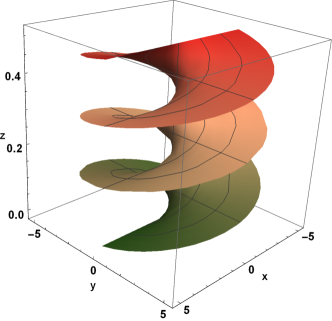
Figure 1 shows a helicoid. The geometric potential in this case is
| (19) |
since the principal curvatures are given by
| (20) |
Our goal consists in considering an harmonic oscillator in a helicoid. This way, the particle will be subjected to an effective potential composed of a geometrical potential for the helicoidal surface and also to an harmonic oscillator potential. Let us construct the hamiltonian. We start by considering the hamiltonian for a particle on a helicoid in the context of anisotropic mass. The corresponding Schrödinger in the coordinates and is
| (21) |
with . Following [46], we make the separation of the variables , where . In addition, the wavefunction normalization demands the transformation [54] in Eq. (21 ).


After these steps, we obtain the Schrödinger equation in the helicoidal geometry:
| (22) |
In particular, if and , we get the potential investigated in Ref. [54]. We already have the Hamiltonian for a particle in a helicoid in the context of anisotropic mass. The next ingredient we need is to include the harmonic oscillator potential to construct an effective potential and write the corresponding differential equation. In Cartesian coordinates, the harmonic potential is given by
| (23) |
where the factor was introduced for convenience.
![[Uncaptioned image]](/html/2005.01210/assets/x6.png)
![[Uncaptioned image]](/html/2005.01210/assets/x7.png)
![[Uncaptioned image]](/html/2005.01210/assets/x8.png)
![[Uncaptioned image]](/html/2005.01210/assets/x9.png) Figure 3: (Color online) A visualization of the effective potential
sketched in Fig. 2-(a).
Figure 3: (Color online) A visualization of the effective potential
sketched in Fig. 2-(a).
![[Uncaptioned image]](/html/2005.01210/assets/x10.png)
![[Uncaptioned image]](/html/2005.01210/assets/x11.png)
![[Uncaptioned image]](/html/2005.01210/assets/x12.png)
![[Uncaptioned image]](/html/2005.01210/assets/x13.png) Figure 4: (Color online) A visualization of the effective potential sketched in Fig. 2-(b).
Figure 4: (Color online) A visualization of the effective potential sketched in Fig. 2-(b).
![[Uncaptioned image]](/html/2005.01210/assets/x14.png)
![[Uncaptioned image]](/html/2005.01210/assets/x15.png)
![[Uncaptioned image]](/html/2005.01210/assets/x16.png)
![[Uncaptioned image]](/html/2005.01210/assets/x17.png) Figure 5: (Color online) A visualization of the effective potential sketched in Fig. 2-(c).
Figure 5: (Color online) A visualization of the effective potential sketched in Fig. 2-(c).
![[Uncaptioned image]](/html/2005.01210/assets/x18.png)
![[Uncaptioned image]](/html/2005.01210/assets/x19.png)
![[Uncaptioned image]](/html/2005.01210/assets/x20.png)
![[Uncaptioned image]](/html/2005.01210/assets/x21.png) Figure 6: (Color online) A visualization of the effective potential sketched in Fig. 2-(d).
Figure 6: (Color online) A visualization of the effective potential sketched in Fig. 2-(d).
We are interested in the motion of an harmonic oscillator with a single frequency , so that the potential (23) written in the coordinates (16) reads as
| (24) |
which can be included into the Eq. (21) by means of the substitution , resulting in the radial equation
| (25) |
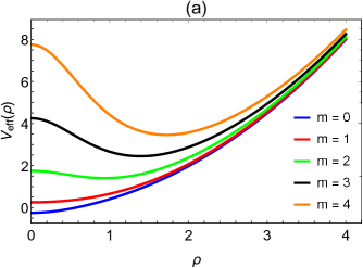
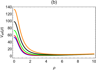
where
| (26) |
is the effective potential. Figure 2 shows plots of , taking some specific values for the effective masses. We consider always being positive, while can be either positive or negative. When , the resulting potential is parabolic for and while for , and it exhibits a narrow binding region (Fig. 2-(a)). These two characteristics have important applications in mesoscopic physics. For example, the former can be considered as a model of a quantum dot while the last one describes a narrow ring. The appearance of these localization regions is a consequence of the helicoidal geometry. However, this characteristic is also manifested when . Figures 2-(b)-(d) clearly show that the presence of anisotropic mass reveals new exotic characteristics for the effective potential. For example, in the particular case when and , a localized wide binding region appears (Fig. 2-(b)). This situation can be interpreted as the analog of a mesoscopic wide ring. Depending on the given anisotropy, more than one binding region may appear. This is exemplified when we have and , which has two binding regions (Fig. 2-(c)). The first located region (near the origin) describes a potential well and the second a wide ring. This model also presents mixed characteristics, such as those present in previous cases. An example of this occurs when and , where we can observe the potential profile present in Figs. 2-(b) and 2-(c). Figures 3-6 show the profiles of Fig. 2, with the exception of the case with , which has an equivalent shape to the curve with in the four cases. The symmetry of the quantum number in the effective potential allows us to visualize more clearly the regions that allow bound states in the figures.
Particularly, the case in which consists of a quantum mechanical analog of a hyperbolic metamaterial, as discussed in [46]. Metamaterials [55] are quite interesting because of their unique possibilities of investigations involving negative refractive indexes and technological developments [56]. Also, metamaterials allow the emulation of theoretical cosmology scenarios in the context of electrodynamics [57]. Thus, basically, it is possible to analyze the harmonic oscillator taking into account three different possibilities: i) an isotropic sample, where the helicoid is surrounded by the same material of the helicoidal surface, ii) an anisotropic material, and iii) an electronic analogue of a hyperbolic material. The effective potential is an even function. This way, the Hamiltonian commutes with the Parity Operator. Then, these operators can share a mutual basis of eigenstates. As a consequence, we expect that the solution can accommodate either symmetric or antisymmetric solutions, like in the case of the commun quantum harmonic oscillator.
Equation (25) can be written as
| (27) |
where , . Equation (27) is of the Heun’s confluent differential equation type [58, 59]
| (28) |
with
| (29) | ||||
| (30) |
The solution to Eq. (28) is computed as a power series expansion around the origin , a regular singular point with a radius of convergence , given by
| (31) |
where the coefficients satisfy a three-term recurrence relation
| (32) |
with initial conditions
| (33) | |||||
| (34) |
where
| (35) | ||||
| (36) | ||||
| (37) |
![[Uncaptioned image]](/html/2005.01210/assets/x22.png)
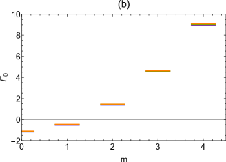
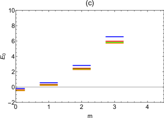
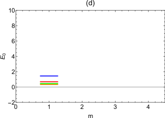
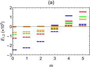
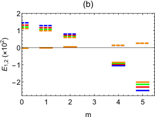
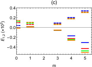
In Table 1, the columns (a)-(d) refer to Figs. 7-8 (a)-(d), respectively. In the order in which the columns are presented, each value pair corresponds to (, ). The colors blue, red, green and orange refer to the energy levels as a function of , following the order in which they appear in the figures.
This confluent Heun function must reduce to a polynomial, since otherwise it would increase exponentially as . To reduce a confluent Heun function to a confluent Heun polynomial of degree we need two successive terms in the three-term recurrence relation, Eq. (32), to vanish, halting the infiniteserie s, Eq. (31). This requirement results in two termination conditions, both needed to be satisfied simultaneously [60, 61, 62, 63]
| (38) | |||
| (39) |
The solution to Eq. (27) is given by
| (40) |
where
| (41) |
We are not interested in situations with . As expected, the solution given by Eq. (40) accommodates both symmetric and antissymmetric eigenstates. In order to obtain the energies, we need to make use of the relations (38) and (39). From condition (38), we obtain
| (42) |

The second termination condition, Eq. (39), for , provides
| (43) |
Substituting Eq. (43) in Eq. (42) and then solving for , we find
| (44) |
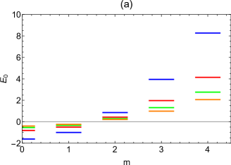
The ground state energy has its minimum shifted as and are varied. The spacing between the levels increases as is increased. (Figure 7 (a)). When assumes ever lower positive values and is kept fixed (column (b) in the Table 1), the minimum energy state is not shifted. (Fig. 7 (b)). When is kept fixed and assumes negative values (column (c) in the Table 1), different from Fig. 7 (a), there is no inversion between levels and, furthermore, the state with is not allowed (Fig. 7 (c)). This characteristic is a consequence of the anisotropic mass. On the other hand, when is fixed and assumes negative values (column (d) in the Table 1), the inversion between levels is absent. However, only the energy with is allowed (Fig. 7 (d)).
For the energy with , the condition (39) requires that
| (45) |
with
| (46) | ||||
| (47) |
The solution of (45) by using Eqs. (29), (30) and (41) provides two values for :
| (48) |
| (49) |
with
| (50) |
and
| (51) |
However, after we replace (48) and (49) in (42) and solve the resulting equation for , we find equal spectra. Thus, we write
| (52) |
| (53) |
with
| (54) | ||||
| (55) |
The energy eigenvalues (52) and (53) present some exotic characteristics manifested by both isotropy and anisotropy in the masses. In the isotropic case, all quantum numbers are allowed (Figure 8 (a)). The energies (52) are responsible for the largest number of negative states while (53) represents only positive states (Figures 8 (b)-(d)). The isotropic mass also reveals that energy states with are nearer when compared to others. In the isotropic case, the relation (52) holds the largest number of states with negative energy while (53) exhibits only positive energy values. This situation is just the opposite of what occurs in the isotropic case. Independent of the values of and , the anisotropic mass affects the full energy states, so that some values of are not allowed (Figures 8 (b)-(d)). This characteristic is typical one of the so-called localized energy states. The appearing of these states is also a consequence of the limitation imposed by the relation (defined in Eq. (41)), which imposes restrictions on the values of and to guarantee that . Besides, we can note that by making some particular choices for the effective masses, we can change how the energy levels are filled. It means, in principle, that these choices could be used to obtain a specific energy profile, filtering the states by their angular momentum . Thus, the geometry and the anisotropy can produce a combined effect in changing the form of the occupation levels.
IV Conclusions
In the present manuscript, we have addressed the motion of a quantum particle on a helicoidal geometry. We have considered the well-established formalism of the geometric potential in the context of anisotropic masses. From the equation for a quantum particle on a helicoid, we have inserted an harmonic oscillator potential into the effective potential through the vector coupling. Then, we calculated the eigenfunctions and energy eigenvalues. These energy eigenvalues are obtained from non-trivial relations since the wavefunction depends on the Confluent Heun Function. In our case, the form of the solution does not allow a negative effective mass , while can be either positive or negative. Despite that, it was possible to consider different configurations with respect to the values of the effective masses. In the case in which both masses are positive, configurations with arbitrary values for and are possible. However, in the case with , it is necessary to be careful: the solution requires . Thus, in the case of an electronic analog of a hyperbolic material in the presence of an harmonic oscillator potential, the anisotropy tends to be larger than in the case of a positive mass . The system can exhibit several different behaviors, depending on the adjustment between the values of the masses. For instance, we have noted that the effective potential can be totally modified by making particular choices for effective masses. In addition, states with different values of angular momentum can be affected differently when subjected to the same type of effective potential. The characteristics observed in the sketch of the effective potential as well as in the energy spectrum allow us to apply this model to others systems in the domain of nanoscale physics, as for example, rings and quantum dots.
Acknowledgments
This work was partially supported by the Brazilian agencies CAPES, CNPq and FAPEMA. EOS acknowledges CNPq Grants 427214/2016-5 and 303774/2016-9, and FAPEMA Grants 01852/14 and 01202/16. MMC acknowledges Coordenação de Aperfeiçoamento de Pessoal de Nível Superior - (CAPES) - Brasil - Grant 88887.358036/2019-00.
References
- Gage Hills et al. [2019] Gage Hills, Christian Lau, Andrew Wright, Samuel Fuller, Mindy D. Bishop, Tathagata Srimani, Pritpal Kanhaiya, Rebecca Ho, Aya Amer, Yosi Stein, et al., Nature 572, 595 (2019).
- Zhuang Liu et al. [2009] Zhuang Liu, Scott Tabakman, Kevin Welsher, and Hongjie Dai, Nano research 2, 85 (2009).
- Kshitij Chaudhary [2013] Kshitij Chaudhary, Int. J. Sci. and Res. (IJSR) 4, 741 (2013).
- Joel E. Moore [2010] Joel E. Moore, Nature 464, 194 (2010).
- Swatantra Kushwaha Kumar Singh et al. [2013] Swatantra Kushwaha Kumar Singh, Saurav Ghoshal, Awani Kumar Rai, and Satyawan Singh, Brazilian Journal of Pharmaceutical Sciences 49, 629 (2013).
- Xiao-Liang Qi and Shou-Cheng Zhang [2011] Xiao-Liang Qi and Shou-Cheng Zhang, Rev. Mod. Phys. 83, 1057 (2011).
- Edward A. Laird et al. [2015] Edward A. Laird, Ferdinand Kuemmeth, Gary A. Steele, Kasper Grove-Rasmussen, Jesper Nygård, Karsten Flensberg, and Leo P. Kouwenhoven, Reviews of Modern Physics 87, 703 (2015).
- Austin Cheng et al. [2019] Austin Cheng, Takashi Taniguchi, Kenji Watanabe, Philip Kim, and Jean-Damien Pillet, arXiv preprint arXiv:1910.13307 (2019).
- Z. Z. Zhang et al. [2008] Z. Z. Zhang, Kai Chang, and F. M. Peeters, Physical review B 77, 235411 (2008).
- H. Sevinçli et al. [2008] H. Sevinçli, Mehmet Topsakal, E. Durgun, and S. Ciraci, Physical Review B 77, 195434 (2008).
- Charles Kane et al. [1997] Charles Kane, Leon Balents, and M. P. A. Fisher, Phys. Rev. Lett. 79, 5086 (1997).
- Jie Yang et al. [2019] Jie Yang, PingAn Hu, and Gui Yu, APL Materials 7, 020901 (2019).
- M. Reza Rezapour et al. [2017] M. Reza Rezapour, Chang Woo Myung, Jeonghun Yun, Amirreza Ghassami, Nannan Li, Seong Uk Yu, Amir Hajibabaei, Youngsin Park, and Kwang S. Kim, ACS applied materials & interfaces 9, 24393 (2017).
- Xitong Liu et al. [2013] Xitong Liu, Mengshu Wang, Shujuan Zhang, and Bingcai Pan, Journal of Environmental Sciences 25, 1263 (2013).
- Minko Balkanski and Ivan Yanchev [2012] Minko Balkanski and Ivan Yanchev, Fabrication, properties and applications of low-dimensional semiconductors, Vol. 3 (Springer Science & Business Media, 2012).
- Thomas Olsen et al. [2018] Thomas Olsen, Erik Andersen, Takuya Okugawa, Daniele Torelli, Thorsten Deilmann, and Kristian S. Thygesen, arXiv preprint arXiv:1812.06666 (2018).
- Andrea C. Ferrari et al. [2015] Andrea C. Ferrari, Francesco Bonaccorso, Vladimir Fal’Ko, Konstantin S. Novoselov, Stephan Roche, Peter Bøggild, Stefano Borini, Frank H. L. Koppens, Vincenzo Palermo, Nicola Pugno, et al., Nanoscale 7, 4598 (2015).
- Liangzhi Kou et al. [2017] Liangzhi Kou, Yandong Ma, Ziqi Sun, Thomas Heine, and Changfeng Chen, The journal of physical chemistry letters 8, 1905 (2017).
- F. H. L. Koppens et al. [2014] F. H. L. Koppens, T. Mueller, Ph Avouris, A. C. Ferrari, M. S. Vitiello, and M. Polini, Nature nanotechnology 9, 780 (2014).
- J. C. D’Olivo and M. Torres [1988] J. C. D’Olivo and M. Torres, Journal of Physics A: Mathematical and General 21, 3355 (1988).
- Ray D’Inverno [1992] Ray D’Inverno, Introducing Einstein’s Relativity (Clarendon Press, 1992).
- Dandoloff et al. [2010] R. Dandoloff, A. Saxena, and B. Jensen, Phys. Rev. A 81, 014102 (2010).
- Rossen Dandoloff [2009] Rossen Dandoloff, Physics Letters A 373, 2667 (2009).
- Victor Atanasov and Rossen Dandoloff [2008] Victor Atanasov and Rossen Dandoloff, Physics Letters A 372, 6141 (2008).
- M. O. Katanaev and I. V. Volovich [1992] M. O. Katanaev and I. V. Volovich, Annals of Physics 216, 1 (1992).
- Fernando Moraes [2000] Fernando Moraes, Brazilian Journal of Physics 30, 304 (2000).
- H. Jensen and H. Koppe [1971] H. Jensen and H. Koppe, Annals of Physics 63, 586 (1971).
- da Costa [1981] R. C. T. da Costa, Phys. Rev. A 23, 1982 (1981).
- da Costa [1982] R. C. T. da Costa, Phys. Rev. A 25, 2893 (1982).
- Giulio Ferrari and Giampaolo Cuoghi [2008] Giulio Ferrari and Giampaolo Cuoghi, Phys. Rev. Lett. 100, 230403 (2008).
- Szameit et al. [2010] A. Szameit, F. Dreisow, M. Heinrich, R. Keil, S. Nolte, A. Tünnermann, and S. Longhi, Phys. Rev. Lett. 104, 150403 (2010).
- DeWitt [1957] B. S. DeWitt, Rev. Mod. Phys. 29, 377 (1957).
- Jurgen Audretsch and V. de Sabbata [2012] Jurgen Audretsch and V. de Sabbata, Quantum mechanics in curved space-time, Vol. 230 (Springer Science & Business Media, 2012).
- Geusa de A. Marques and Valdir B. Bezerra [2002] Geusa de A. Marques and Valdir B. Bezerra, Phys. Rev. D 66, 105011 (2002).
- Bruschi et al. [2014] D. E. Bruschi, T. C. Ralph, I. Fuentes, T. Jennewein, and M. Razavi, Phys. Rev. D 90, 045041 (2014).
- M. G. Burt [1992] M. G. Burt, Journal of Physics: Condensed Matter 4, 6651 (1992).
- De Matteis et al. [2019] G. De Matteis, L. Martina, C. Naya, and V. Turco, Phys. Rev. E 100, 052703 (2019).
- Ludmila V. Yakushevich [2006] Ludmila V. Yakushevich, Nonlinear Physics of DNA (John Wiley & Sons, 2006) Chap. 1, pp. 1–17.
- Maria Barbi et al. [1999] Maria Barbi, Simona Cocco, and Michel Peyrard, Physics Letters A 253, 358 (1999).
- Brian Ribbans et al. [2016] Brian Ribbans, Yujie Li, and Ting Tan, Journal of the mechanical behavior of biomedical materials 56, 57 (2016).
- Jay Armas and Matthias Blau [2015] Jay Armas and Matthias Blau, Journal of High Energy Physics 2015, 48 (2015).
- Frank Wassmann and Adrian Ankiewicz [1998] Frank Wassmann and Adrian Ankiewicz, Appl. Opt. 37, 3902 (1998).
- Masataka Watanabe et al. [2015] Masataka Watanabe, Hisato Komatsu, Naoto Tsuji, and Hideo Aoki, Phys. Rev. B 92, 205425 (2015).
- Haifei Zhan et al. [2017] Haifei Zhan, Yingyan Zhang, Chunhui Yang, Gang Zhang, and Yuantong Gu, Carbon 120, 258 (2017).
- Victor Atanasov et al. [2009] Victor Atanasov, Rossen Dandoloff, and Avadh Saxena, Physical Review B 79, 033404 (2009).
- Pedro H. Souza et al. [2018] Pedro H. Souza, Edilberto O. Silva, Moises Rojas, and Cleverson Filgueiras, Annalen der Physik 530, 1800112 (2018).
- M. Sebawe Abdalla and Hichem Eleuch [2016] M. Sebawe Abdalla and Hichem Eleuch, AIP Advances 6, 055011 (2016).
- R. Yukawa et al. [2015] R. Yukawa, K. Ozawa, S. Yamamoto, R. -Y. Liu, and I. Matsuda, Surface Science 641, 224 (2015).
- R. C. T. da Costa [1981] R. C. T. da Costa, Phys. Rev. A 23, 1982 (1981).
- J. Holland and University [2013] J. Holland and A. N. University, Weingarten Curvature Equations (Australian National University, 2013).
- J. A. Vinasco et al. [2018] J. A. Vinasco, A. Radu, E. Kasapoglu, R. L. Restrepo, A. L. Morales, E. Feddi, M. E. Mora-Ramos, and C. A. Duque, Scientific Reports 8, 13299 (2018).
- Robert F. Pierret and Gerold W. Neudeck [1987] Robert F. Pierret and Gerold W. Neudeck, Advanced semiconductor fundamentals, Vol. 6 (Addison-Wesley Reading, MA, 1987).
- A. Gray [1993] A. Gray, Modern Differential Geometry of Curves and Surfaces (Boca Raton: CRC Press, 1993).
- Atanasov et al. [2009] V. Atanasov, R. Dandoloff, and A. Saxena, Phys. Rev. B 79, 033404 (2009).
- D. R. Smith et al. [2004] D. R. Smith, J. B. Pendry, and M. C. K. Wiltshire, Science 305, 788 (2004).
- Ruopeng Liu et al. [2015] Ruopeng Liu, Chunlin Ji, Zhiya Zhao, and Tian Zhou, Engineering 1, 179 (2015).
- David Figueiredo et al. [2017] David Figueiredo, Fernando Moraes, Sébastien Fumeron, and Bertrand Berche, Phys. Rev. D 96, 105012 (2017).
- F. M. Arscott et al. [1995] F. M. Arscott, Slavyanov S. Yu., D. Schmidt, G. Wolf, P. Maroni, and A. Duval, Heun’s Differential Equations, Oxford science publications (Oxford University Press, 1995).
- Sergei Yu. Slavyanov and Wolfgang Lay [2000] Sergei Yu. Slavyanov and Wolfgang Lay, Special Functions: A Unified Theory Based on Singularities, Oxford mathematical monographs (Oxford University Press, 2000).
- C. A. Downing and M. E. Portnoi [2016] C. A. Downing and M. E. Portnoi, Phys. Rev. B 94, 165407 (2016).
- C. A. Downing [2013] C. A. Downing, Journal of Mathematical Physics 54, 072101 (2013).
- Plamen P. Fiziev [2009a] Plamen P. Fiziev, Phys. Rev. D 80, 124001 (2009a).
- Plamen P. Fiziev [2009b] Plamen P. Fiziev, Journal of Physics A: Mathematical and Theoretical 43, 035203 (2009b).