Riemannian Stochastic Proximal Gradient Methods for Nonsmooth Optimization over the Stiefel Manifold

Abstract

Riemannian optimization has drawn a lot of attention due to its wide applications in practice. Riemannian stochastic first-order algorithms have been studied in the literature to solve large-scale machine learning problems over Riemannian manifolds. However, most of the existing Riemannian stochastic algorithms require the objective function to be differentiable, and they do not apply to the case where the objective function is nonsmooth. In this paper, we present two Riemannian stochastic proximal gradient methods for minimizing nonsmooth function over the Stiefel manifold. The two methods, named R-ProxSGD and R-ProxSPB, are generalizations of proximal SGD and proximal SpiderBoost in Euclidean setting to the Riemannian setting. Analysis on the incremental first-order oracle (IFO) complexity of the proposed algorithms is provided. Specifically, the R-ProxSPB algorithm finds an $\epsilon$-stationary point with $\mathcal{O}(\epsilon^{-3})$ IFOs in the online case, and $\mathcal{O}(n+\sqrt{n}\epsilon^{-2})$ IFOs in the finite-sum case with $n$ being the number of summands in the objective. Experimental results on online sparse PCA and robust low-rank matrix completion show that our proposed methods significantly outperform the existing methods that use Riemannian subgradient information.

Keywords: Riemannian Optimization, Stochastic Gradient Descent, SPIDER, Manifold Proximal Gradient Method, Online Sparse PCA

1 Introduction

We consider the following composite optimization problem over the Stiefel manifold $\mathcal{M}:=\mathrm{St}(d,r)=\{X\in\mathbb{R}^{d\times r}\mid X^{\top}X=I_{r}\}$:

$$\min_{X\in\mathcal{M}}F(X):=f(X)+h(X),$$ (1)

where $f(X)$ takes one of the following two forms:

• Online case:

  $$f(X):=\mathbb{E}_{\pi}[f(X;\pi)],$$ (2)

  where $\mathbb{E}_{\pi}$ is the expectation with respect to the random variable $\pi$.

• Finite-sum case:

  $$f(X):=\frac{1}{n}\sum_{i=1}^{n}f_{i}(X),$$ (3)

  where $n$ denotes the number of data and is assumed to be extremely large.

Throughout this paper, we assume that $f(\cdot;\pi)$, $f_{i}(\cdot)$ and thus $f(\cdot)$ are all smooth, $h$ is convex and possibly nonsmooth. Here the smoothness and convexity are interpreted when the function in question is considered as a function in the ambient Euclidean space. Note that since (2) involves an expectation, and (3) involves extremely large $n$, we assume that the full gradient information of $f$ is not available and only stochastic estimators to the gradient of $f$ can be obtained.

Problem (1) with $f$ being (2) and (3) appears frequently in machine learning applications. In the online case (2), $f(X;\pi)$ denotes the loss function corresponding to data $\pi$; and in the finite-sum case (3), $f_{i}(X)$ denotes the loss function corresponding to the $i$-th sample data. Function $h$ is usually a regularizer that can promote certain desired structure of the solution. For example, letting $h(X)=\|X\|_{1}:=\sum_{ij}|X_{ij}|$ serves the purpose of promoting the sparsity of solution $X$.

One important application of (1) in the online case is the online sparse PCA, which can be cast as

$$\min_{X}\quad\mathbb{E}_{Z\in\mathcal{D}}[\|Z-XX^{\top}Z\|_{2}^{2}]+\mu\|X\|_{1},\textrm{s.t.},X\in\mathcal{M},$$ (4)

where $\mu>0$ is a weighting parameter, $\mathcal{D}$ denotes the distribution of the random online data $Z$, and the $\ell_{1}$ norm is used to promote the sparsity of the eigenvectors. In this case, $r$ is the desired number of principal components. For PCA, each principal component is a linear combination of all variables, and it is usually difficult to interpret the derived principal components, especially when the dimension is high. Simple thresholding is an ad hoc way to estimate sparse loadings for better interpretability, but it may result in misleading results in various respects (Cadima and Jolliffe, 1995). By solving a manifold optimization problem, sparse PCA estimates sparse loadings to achieve a good balance between dimension reduction and interpretability. Sparse PCA has been widely used in many research fields such as medical imaging, ecology, and neuroscience. In the landmark-based shape analysis of the CC brain structure, Sjostrand et al. (2007) found that sparse PCA is useful to derive localized and interpretable patterns of variability while PCA did not provide much interpretational value. Gravuer et al. (2008) applied sparse PCA to perform the dimension reduction before fitting the aggregated boosted trees model, and the sparsity helps the interpretability of their model. Recently, Baden et al. (2016) used sparse PCA to study the functional diversity of mouse retinal ganglion cells through a clustering framework and found that SPCA leads to better cluster quality than PCA. Although PCA and sparse PCA have been studied extensively in the literature, studies for online sparse PCA, i.e., sparse PCA with streaming data, seem to be very limited (Yang and Xu, 2015; Wang and Lu, 2016). In this paper, we propose efficient stochastic Riemannian algorithms for solving this important application.

1.1 Related Works

Riemannian optimization has been an active research area in the last decade, due to its wide applications in machine learning, signal processing, statistics and so on. The monograph by Absil et al. (2009) studied optimization algorithms on matrix manifolds in depth. Recently, Riemannian optimization with nonsmooth objective has attracted a lot of attention due to its applications in sparse PCA (Jolliffe et al., 2003), compressed modes in physics (OzoliņVs et al., 2013), unsupervised feature selection (Yang et al., 2011; Tang and Liu, 2012), sparse blind deconvolution (Zhang et al., 2017), to name just a few. Many deterministic algorithms for solving Riemannian optimization with nonsmooth objective have been studied recently, including Riemannian subgradient method (Li et al., 2019), manifold proximal gradient method (ManPG) (Chen et al., 2020b), Riemannian proximal gradient method (Huang and Wei, 2019), manifold proximal point algorithm (Chen et al., 2020a), manifold proximal linear algorithm (Wang et al., 2021) and so on. When the loss function $f$ takes the expectation or finite-sum form as in (2) and (3), stochastic algorithms are usually in demand because we have only access to noisy stochastic gradients of $f$ instead of the full gradient. When the nonsmooth regularizer $h$ vanishes, that is, when (1) reduces to a smooth problem with $f$ given by (2) or (3), there exist stochastic algorithms for solving it. In particular, R-SGD (Bonnabel, 2013), R-SVRG (Zhang and Sra, 2016), R-SRG (Kasai et al., 2018) and R-SPIDER (Zhou et al., 2019; Zhang et al., 2018) can all be used to solve it. Among these algorithms, R-SVRG, R-SRG and R-SPIDER all utilize the variance reduction techniques (Johnson and Zhang, 2013; Defazio et al., 2014) to improve the convergence rate of R-SGD. On the other hand, when the nonsmooth regularizer $h$ presents but the manifold constraint vanishes in (1), i.e., when $\mathcal{M}$ is the Euclidean space, there exist stochastic proximal gradient algorithms for solving these unconstrained problems in Euclidean space. Popular methods include ProxSGD (Rosasco et al., 2014), ProxSVRG (Xiao and Zhang, 2014), ProxSARAH (Pham et al., 2019) and ProxSpiderBoost (Wang et al., 2019). However, to the best of our knowledge, when both nonsmooth regularizer $h$ and manifold constraint $X\in\mathcal{M}$ present as in (1), there is no stochastic algorithm that can solve them. In this paper, we close this gap by proposing two stochastic algorithms, namely R-ProxSGD and R-ProxSPB, for solving (1) with $f$ being (2) or (3), i.e., Riemannian optimization with nonsmooth objectives. Our algorithms are inspired by the ManPG algorithm that is recently proposed by Chen et al. (2020b) for solving the nonsmooth Riemannian optimization problem (1). ManPG assumes that the full gradient of $f$ can be obtained, and thus it is a deterministic algorithm, while our R-ProxSGD and R-ProxSPB are the first stochastic algorithms for solving (1) without using subgradient information. Recently, Li et al. (2019) showed that when the objective function is weakly convex, Riemannian stochastic subgradient Method (R-Subgrad) has $\mathcal{O}(\epsilon^{-4})$ iteration complexity for obtaining an $\epsilon$-stationary point.

Objective	Euclidean	Riemannian
Smooth	SGD (Nemirovski et al., 2009)	R-SGD (Bonnabel, 2013)
	SVRG (Johnson and Zhang, 2013)	R-SVRG (Zhang and Sra, 2016)
	SARAH (Nguyen et al., 2017)	R-SRG (Kasai et al., 2018)
	SPIDER (Fang et al., 2018)	R-SPIDER (Zhou et al., 2019; Zhang et al., 2018)
	SpiderBoost (Wang et al., 2019)	R-SpiderBoost (ours)
	ProxSGD (Rosasco et al., 2014)	R-ProxSGD (ours)
Non-	ProxSVRG (Xiao and Zhang, 2014)	N/A
smooth	ProxSARAH (Pham et al., 2019)	N/A
	ProxSpiderBoost (Wang et al., 2019)	R-ProxSPB (ours)

Table 1: Summary of existing methods and our methods in Euclidean and Riemannian settings.

Algorithms	Step size	Finite-sum	Online
ManPG (Chen et al., 2020b)	constant	$\mathcal{O}(n\epsilon^{-2})$	N/A
R-ProxSGD	constant	N/A	$\mathcal{O}(\epsilon^{-4})$
R-ProxSPB	constant	$\mathcal{O}(n+\sqrt{n}\epsilon^{-2})$	$\mathcal{O}(\epsilon^{-3})$

Table 2: Comparison of IFO complexity for nonsmooth Riemannian optimization methods over the Stiefel manifold.

1.2 Our Contributions

The contributions of this paper lie in several folds.

1. First, we propose two stochastic algorithms for solving (1). These two algorithms, named R-ProxSGD and R-ProxSPB, are Riemannian generalizations of their counterparts in the Euclidean setting: ManPG (Chen et al., 2020b) and ProxSpiderBoost (Wang et al., 2019). On the other hand, they can also be viewed as generalizations of their smooth counterparts, R-SGD and R-SpiderBoost, to the nonsmooth case. However, we emphasize here that although the design of these algorithms are straightforward, proving their convergence is more involved, due to the presence of stochastic gradients information. In Table 1 we give a summary of existing methods and our proposed methods in different cases: the objective is smooth or nonsmooth and the constraint is Riemannian manifold or Euclidean space. Note that when the nonsmooth function $h$ vanishes, our R-ProxSPB reduces to a Riemannian SpiderBoost algorithm (R-SpiderBoost) that solves Riemannian optimization with smooth objective. It seems that R-SpiderBoost is also new in the literature.

2. Second, we prove the convergence of the proposed two algorithms and analyze their incremental first-order oracle (IFO) complexity results. Specifically, we analyze the IFO complexity of R-ProxSGD for the online setting problem, i.e., (1) with $f$ being (2); and R-ProxSPB for both the online setting problem and the finite-sum setting problem, i.e., (1) with $f$ being (3). In Table 2 we summarize the IFO complexity results of our proposed algorithms and the existing ManPG algorithm, as they are the only algorithms that can solve the nonsmooth Riemannian optimization problem (1) with known IFO complexity results.

3. Third, we conduct numerical experiments for solving online sparse PCA (4) and robust low-rank matrix completion problems to demonstrate the advantages of the proposed methods.

Remark 1

We provide some further remark about the proposed algorithms R-ProxSGD and R-ProxSPB. Our algorithms incorporated several concepts, including Riemannian algorithm, proximal algorithm, stochastic algorithm, and variance reduction. We point out that they are all well motivated and justified. Note that the problem (1) has three items that need to be taken care of: the manifold constraint, the smooth function $f$ and the nonsmooth function $h$. First, to deal with the manifold constraint, a Riemannian algorithm needs to be adopted. Second, since we do not have access to the full gradient information of the smooth function $f$, we need to design a stochastic algorithm that utilizes the noisy gradient information only. Third, to handle the nonsmooth function $h$, we need to design a proximal algorithm. Last, the variance reduction technique is adopted to reduce the variance of the stochastic gradients, and thus to accelerate the convergence of the algorithm.

Organization. The rest of the paper is organized as follows. Section 2 introduces the necessary notation and assumptions. Our new algorithms and their convergence and complexity results are presented in Section 3. The experimental results are reported in Section 4. Finally, we make some concluding remarks in Section 5. The detailed proofs of the theorems and lemmas are provided in the appendix.

2 Preliminaries

In this work, we consider the Riemannian submanifold $(\mathcal{M},\mathfrak{g})$ where $\mathcal{M}$ is the Stiefel manifold and $\mathfrak{g}$ is the Riemannian metric on $\mathcal{M}$ that is induced from the Euclidean inner product. That is, for any $x\in\mathcal{M}$, $\xi\in\mathrm{T}_{x}\mathcal{M}$ and $\zeta\in\mathrm{T}_{x}\mathcal{M}$, we have $\langle\xi,\zeta\rangle_{x}=\langle\xi,\zeta\rangle$, where $\mathrm{T}_{x}\mathcal{M}$ denotes the tangent space of $\mathcal{M}$ at $x$. For smooth function $f$, we use $\mathrm{grad}f(X)$ to denote the full Riemannian gradient of $f$ at $X$, and $\nabla f({X})$ represents the full Euclidean gradient of $f$ at $X$. With an abuse of notation, when there is no ambiguity, we use $f_{i}$ to denote the component function in the online case (2), i.e., $f_{i}(X):=f(X;\pi_{i})$, though it is still used as a component function in the finite-sum case (3). For a mini-batch set $\mathcal{S}$, $\nabla f_{\mathcal{S}}(X):=\frac{1}{|\mathcal{S}|}\sum_{i\in\mathcal{S}}\nabla f_{i}(X)$ denotes the stochastic Euclidean gradient estimated on $\mathcal{S}$. We use $\mathcal{F}_{t}$ to denote all randomness occurred up to (include) the $t$-th iteration of any algorithm. When there is no ambiguity, we use $\|\mathbf{a}\|$ to denote the Frobenius norm when $\mathbf{a}$ is a matrix and the Euclidean norm when $\mathbf{a}$ is a vector.

A classical geometric concept in the study of manifolds is the exponential mapping, which defines a geodesic curve on the manifold. However, the exponential mapping is difficult to compute in general. The concept of a retraction (Absil et al., 2009), which is a first-order approximation of the exponential mapping and can be more amenable to computation, is given as follows.

Definition 2

(Absil et al., 2009, Definition 4.1.1) A retraction on a differentiable manifold $\mathcal{M}$ is a smooth mapping Retr from the tangent bundle $\mathrm{T}\mathcal{M}$ onto $\mathcal{M}$ satisfying the following two conditions (here $\textrm{Retr}_{X}$ denotes the restriction of Retr onto $\mathrm{T}_{X}\mathcal{M}$):

1. $\textrm{Retr}_{X}(0)=X,\forall X\in\mathcal{M}$, where $0$ denotes the zero element of $\mathrm{T}_{X}\mathcal{M}$.

2. For any $X\in\mathcal{M}$, it holds that

   $$\lim_{\mathrm{T}_{X}\mathcal{M}\ni\xi\rightarrow 0}\frac{\|\textrm{Retr}_{X}(\xi)-(X+\xi)\|}{\|\xi\|}=0.$$

Remark 3

Here and thereafter, when we talk about the summation $X+\xi$, we always treat $X$ and $\xi$ as elements in the ambient Euclidean space so that their sum is well defined. The second condition in Definition 2 ensures that $\textrm{Retr}_{X}(\xi)=X+\xi+\mathcal{O}(\|\xi\|^{2})$ and $D\textrm{Retr}_{X}(0)=\mathrm{Id}$, where $D\textrm{Retr}_{X}$ is the differential of $\textrm{Retr}_{X}$ and $\mathrm{Id}$ denotes the identity mapping. For more details about retraction, we refer the reader to Absil et al. (2009); Boumal et al. (2019) and the references therein.

The retraction onto the Euclidean space is simply the identity mapping; i.e., $\textrm{Retr}_{X}(\xi)=X+\xi$. For the Stiefel manifold $\mathrm{St}(d,r)$, common retractions include the exponential mapping (Edelman et al., 1999)

$$\textrm{Retr}_{X}^{\mathrm{exp}}(\xi)=[X,Q]\exp\left(\begin{bmatrix}-X^{\top}\xi&-R^{\top}\\ R&0\end{bmatrix}\right)\begin{bmatrix}I_{r}\\ 0\end{bmatrix},$$

where $QR=-(I_{d}-XX^{\top})\xi$ is the unique QR factorization; the polar decomposition

$$\textrm{Retr}_{X}^{\mathrm{polar}}(\xi)=(X+\xi)(I_{r}+\xi^{\top}\xi)^{-1/2};$$

the QR decomposition

$$\textrm{Retr}_{X}^{\mathrm{QR}}(\xi)=\mathrm{qf}(X+\xi),$$

where $\mathrm{qf}(A)$ is the $Q$ factor of the QR factorization of $A$; the Cayley transformation (Wen and Yin, 2013)

$$\textrm{Retr}_{X}^{\mathrm{cayley}}(\xi)=\left(I_{d}-\frac{1}{2}W(\xi)\right)^{-1}\left(I_{d}+\frac{1}{2}W(\xi)\right)X,$$

where $W(\xi)=(I_{d}-\frac{1}{2}XX^{\top})\xi X^{\top}-X\xi^{\top}(I_{d}-\frac{1}{2}XX^{\top})$.

In this paper, we adopt the assumption that the retraction that we use is invertible, the same as what is assumed in existing works (Kasai et al., 2018; Zhou et al., 2019). We use $\Gamma_{X}^{Y}$ to denote the vector transport from $X$ to $Y$ satisfying $\textrm{Retr}_{X}{(\xi)}=Y$. Vector transport $\Gamma:\mathrm{T}\mathcal{M}\bigoplus\mathrm{T}\mathcal{M}\rightarrow\mathrm{T}\mathcal{M}$, $(\xi,\zeta)\mapsto\Gamma_{X}^{Y}(\zeta)$ is associated with the retraction Retr, where $\xi,\zeta\in\mathrm{T}_{X}\mathcal{M}$.

The following assumptions regarding the retraction and vector transport are necessary to our analysis.

Assumption 4

1. (see Kasai et al. (2018)). All of the iterates $\{X_{t}\}_{t=1}^{T+1}$ are in a totally retractive neighborhood $\mathcal{U}\subset\mathcal{M}$ of an optimum $X^{*}$: $\{\mathrm{Retr}_{X_{t}}(\xi_{t})\}\in\mathcal{U}$ with $X_{t+1}=\mathrm{Retr}_{X_{t}}(\zeta_{t})$, $\zeta_{t}\in\mathrm{T}_{X_{t}}\mathcal{M}$.

2. (see Kasai et al. (2018)). Suppose that $\mathrm{Exp}_{X}:\mathrm{T}_{X}\mathcal{M}\rightarrow\mathcal{M}$ denotes the exponential mapping and $\mathrm{Exp}_{X}^{-1}:\mathcal{M}\rightarrow\mathrm{T}_{X}\mathcal{M}$ is its inverse mapping. There exist $c_{R},c_{E}>0$ such that $\|\mathrm{Exp}_{X}^{-1}(Y)-\mathrm{Retr}_{X}^{-1}(Y)\|\leq c_{R}\|\mathrm{Retr}_{X}^{-1}(Y)\|$, $\forall X,Y\in\mathcal{U}$ and $\|\textrm{Retr}_{X}^{-1}(Y)\|\leq c_{E}\|\xi\|$ if $\textrm{Retr}_{X}(\xi)=Y$.

3. (see Boumal et al. (2019)). For all $X\in\mathcal{M}$ and $\xi\in\mathrm{T}_{X}\mathcal{M}$, there exist constants $M_{1}>0$ and $M_{2}>0$ such that the following two inequalities hold:

   $$\|\mathrm{Retr}_{X}(\xi)-X\|\leq M_{1}\|\xi\|$$ (5)

   $$\|\mathrm{Retr}_{X}(\xi)-(X+\xi)\|\leq M_{2}\|\xi\|^{2}.$$ (6)

4. $f(\cdot;\pi)$, $f_{i}(\cdot)$ and $f(\cdot)$ are all twice continuously differentiable.

Assumption 5

(see Kasai et al. (2018)). The vector transport is isometric on the manifold $\mathcal{M}$, i.e., $\|\Gamma_{X}^{Y}(\zeta)\|=\|\zeta\|$ for $X,Y\in\mathcal{M}$, $\xi,\zeta\in\mathrm{T}_{X}\mathcal{M}$ and $\textrm{Retr}_{X}{(\xi)}=Y$.

Besides, we impose some assumptions on $f(X)$ and its first-order oracle, which are also required in previous work on smooth Riemannian optimization with retraction and vector transport (Kasai et al., 2018; Zhou et al., 2019).

Assumption 6 (Upper-bounded Hessian of $f$)

Every individual loss $f_{i}(X)$ is twice continuously differentiable and the individual Hessian of every $f_{i}(X)$ is bounded as $\|\nabla^{2}f_{i}(X)\|\leq L_{H}$. $f(X)$ has upper-bounded Hessian in $\mathcal{U}\in\mathcal{M}$ with respect to the retraction $\mathrm{Retr}_{X}(\cdot)$ if there exists $L_{R}>0$ such that $\frac{d^{2}f(\mathrm{Retr}_{X}(t\xi))}{dt^{2}}\leq L_{R}$ for all $X\in\mathcal{U},\xi\in\mathrm{T}_{X}\mathcal{M}$ with $\|\xi\|=1$ and all $t$ such that $\mathrm{Retr}_{X}(\tau\xi)\in\mathcal{U}$ for all $\tau\in[0,t]$.

Assumption 7 (Bounded variance)

Stochastic gradient oracle of every individual loss $f_{i}(X)$ is bounded $\|\nabla f_{i}(X)\|\leq G$ and its variance is also bounded $\mathbb{E}_{i}[\|\nabla f_{i}(X)-\nabla f(X)\|^{2}]\leq\sigma^{2}$.

Moreover, we make the following assumption on the regularization term $h(X)$.

Assumption 8

The regularization function $h$ is convex and $L_{h}$-Lipschitz continuous, i.e., $\|h(X)-h(Y)\|\leq L_{h}\|X-Y\|$, $\forall X,Y\in\mathcal{M}$.

We now give the definition of the stationary point of problem (1), which is standard in the literature, see (Yang et al., 2014; Chen et al., 2020b).

Definition 9 (Stationary point)

$X\in\mathcal{M}$ is a stationary point of (1) if it satisfies:

$$0\in\hat{\partial}F(X):={\mathrm{{grad}}f(X)}+\mathrm{Proj}_{\mathrm{T}_{X}\mathcal{M}}{\partial}h(X),$$ (7)

where $\mathrm{{grad}}f(X)$ is the Riemannian gradient of $f$ at $X$, and $\hat{\partial}F(X)$ is the generalized Clarke subdifferential at $X$ (see Definition 17 in Appendix).

The computational costs of the algorithms are evaluated in terms of IFO complexity.

Definition 10

An IFO takes an index $i\in\{1,\ldots,n\}$ and returns $(f_{i}(X),\nabla f_{i}(X))$ for the finite-sum case (3), or $(f(X;\pi_{i}),\nabla_{X}f(X;\pi_{i}))$ for the online case (2).

3 Riemannian Stochastic Proximal Gradient Methods

In this section, we introduce our Riemannian stochastic proximal gradient algorithms and provide their non-asymptotic convergence results. Proofs of the theorems are provided in the appendix.

3.1 The Main Framework

The main framework of our Riemnannian stochastic proximal gradient algorithms is inspired by the ManPG algorithm (Chen et al., 2020b). The ManPG algorithm aims to solve the nonsmooth Riemannian optimization problem (1) by assuming that the full gradient of $f$ can be accessed. Therefore, it is a deterministic algorithm. ManPG is a generalization of the proximal gradient method from Euclidean setting to the Riemannian setting. The proximal gradient method for solving $\min_{X}F(X):=f(X)+h(X)$ in the Euclidean setting generates the iterates as follows:

$$X_{t+1}:=\mathop{\mathrm{argmin}}_{Y}f(X_{t})+\langle\nabla f(X_{t}),Y-X_{t}\rangle+\frac{1}{2\gamma}\|Y-X_{t}\|^{2}+h(Y).$$ (8)

In other words, one minimizes the quadratic function $Y\mapsto f(X_{t})+\langle\nabla f(X_{t}),Y-X_{t}\rangle+\frac{1}{2\gamma}\|Y-X_{t}\|^{2}+h(Y)$ of $F$ at $X_{t}$ in the $t$-th iteration, where $\gamma>0$ is a parameter that can be regarded as the stepsize. It is known that this quadratic function can bound $F$ from above when $\gamma\leq 1/L$, where $L$ is the Lipschitz constant of $\nabla f$. The subproblem (8) corresponds to the proximal mapping of $h$ and the efficiency of the proximal gradient method relies on the assumption that (8) is easy to solve. For (1), in order to deal with the manifold constraint, one needs to ensure that the descent direction lies in the tangent space. This motivates the following subproblem for finding the descent direction $\xi_{t}$ in the $t$-th iteration:

$$\begin{array}[]{ll}\mathbf{\xi}_{t}=&\mathop{\mathrm{argmin}}_{\mathbf{\xi}}:=\langle\nabla f(X_{t}),\mathbf{\xi}\rangle+\frac{1}{2\gamma}\|\mathbf{\xi}\|^{2}+h(X_{t}+\mathbf{\xi})\\ &\mathrm{s.t.}\quad\mathbf{\xi}\in\mathrm{T}_{X_{t}}\mathcal{M},\end{array}$$ (11)

and then a retraction step is performed to keep the iterate feasible to the manifold constraint:

$$X_{t+1}:=\textrm{Retr}_{X_{t}}(\eta_{t}\xi_{t}).$$ (12)

It is shown that the ManPG algorithm (11)-(12) finds an $\epsilon$-stationary point of (1) in $O(\epsilon^{-2})$ iterations. It was shown in (Chen et al., 2020b) that ManPG performs better than some existing algorithms for solving the sparse PCA problem. The ManPG algorithm was extended successfully later to solving problems with two block variables (Chen et al., 2020c) such as another sparse PCA formulation (Zou et al., 2006) and the sparse CCA problem (Hardoon and Shawe-Taylor, 2011).

Motivated by the success of the ManPG algorithm, when we only have the access to stochastic gradient of $f$, we design a stochastic version of ManPG to solve (1). In particular, each iteration of our proposed algorithm consists of two steps: (i) finding the descent direction, and (ii) performing retraction. The basic framework of our proposed algorithm is to simply replace the full gradient in ManPG by a stochastic estimator to the gradient. This leads to the following updating scheme of the proposed framework:

$$\begin{array}[]{ll}\mathbf{\zeta}_{t}=&\mathop{\mathrm{argmin}}_{\mathbf{\zeta}}\phi_{t}(\mathbf{\zeta})\!:=\!\langle V_{t},\mathbf{\zeta}\rangle+\frac{1}{2\gamma}\|\mathbf{\zeta}\|^{2}+h(X_{t}+\mathbf{\zeta})\\ &\mathrm{s.t.}\quad\mathbf{\zeta}\in\mathrm{T}_{X_{t}}\mathcal{M},\end{array}$$ (15)

and

$$X_{t+1}:=\textrm{Retr}_{X_{t}}(\eta_{t}\mathbf{\zeta}_{t}),$$ (16)

where $\gamma>0$ and $\eta_{t}>0$ are step sizes, and $V_{t}$ denotes a stochastic estimation of the Euclidean gradient $\nabla f(X_{t})$. Specific choices of $V_{t}$ will be discussed in Sections 3.2 and 3.3. Note that for the Stiefel manifold $\mathcal{M}$, the tangent space is given by $\mathrm{T}_{X}\mathcal{M}=\{\zeta\mid\zeta^{\top}X+X^{\top}\zeta=0\}$. Therefore, the constraint in (15) is a linear equality constraint. Since we assume that $h$ is a convex function, it follows that the subproblem (15) is a convex problem. This convex problem can be efficiently solved using the semi-smooth Newton method (Xiao et al., 2018). We refer the readers to Xiao et al. (2018) and Chen et al. (2020b) for more details on how to solve (15) efficiently.

To prepare for the analysis of IFO complexity, we need to define the $\epsilon$-stationary solution and the $\epsilon$-stochastic stationary point.

Definition 11 ($\epsilon$-stationary point and $\epsilon$-stochastic stationary point)

Define

$$G(X,\nabla f(X),\gamma)=(X-\mathrm{Retr}_{X}(\xi))/\gamma,$$ (17)

where

$$\xi:=\mathop{\mathrm{argmin}}_{\xi\in\mathrm{T}_{X}\mathcal{M}}\{\langle\nabla f(X),\xi\rangle+\frac{1}{2\gamma}\|\xi\|^{2}+h(X+\xi)\}.$$ (18)

$X$ is called an $\epsilon$-stationary point of (1) if $\|G(X,\nabla f(X),\gamma)\|\leq\epsilon$. When the sequence $\{X_{t}\}$ is generated by a stochastic algorithm (stochastic process), we call $X_{t}$ an $\epsilon$-stochastic stationary point if $\mathbb{E}[\|G(X_{t},\nabla f(X_{t}),\gamma)\|]\leq\epsilon$, where the expectation $\mathbb{E}$ is taken for all randomness before $X_{t}$ is generated.

Remark 12

Note that $\xi$ defined in (18) is the solution to (15) with full gradient $V_{t}=\nabla f(X_{t})$. In the Euclidean space, $\textrm{Retr}_{X_{t}}(\gamma\xi_{t})$ reduces to $X_{t}+\gamma\xi_{t}$ and $\xi_{t}=\mathrm{prox}_{\gamma h}(X_{t}-\gamma\nabla f(X))-X$. Thus, $G(X_{t},\nabla f(X_{t}),\gamma)$ defined in (17) is analogous to the proximal gradient in the Euclidean space.

3.2 R-ProxSGD: Riemannian Stochastic Proximal Gradient Descent Algorithm

In this section, we design the basic Riemannian proximal stochastic gradient descent method (R-ProxSGD) by choosing $V_{t}$ as the mini-batch stochastically sampled gradients. More specifically, in the $t$-th iteration of R-ProxSGD, we randomly sample a mini-batch set $\mathcal{S}_{t}$, and define $V_{t}=\frac{1}{|\mathcal{S}_{t}|}\sum_{{i_{t}}\in\mathcal{S}_{t}}\nabla f_{i_{t}}(X_{t})$, which is an unbiased gradient estimator with bounded variance. That is, $\mathbb{E}[V_{t}]=\nabla f(X_{t})$ and $\mathbb{E}[\|V_{t}-\nabla f(X_{t})\|^{2}]\leq\frac{\sigma^{2}}{|\mathcal{S}_{t}|}$. Our R-ProxSGD is described in Algorithm 1.

Algorithm 1 R-ProxSGD

1:  Input: initial point $X_{0}\in\mathcal{M}$, parameters $\eta\in(0,1)$,

$$\gamma=\frac{2\eta}{2\tilde{L}\eta^{2}+\eta+1},\quad\mbox{where}\quad\tilde{L}=L_{R}/2+L_{h}M_{2}.$$ (19)

2:  for $t=0,1,...,T-1$ do

3:     Compute the stochastic gradient by randomly sampling a mini-batch set $\mathcal{S}_{t}$ and calculating the unbiased stochastic gradient estimator:

$$V_{t}=\nabla f_{\mathcal{S}_{t}}(X_{t}):=\frac{1}{|\mathcal{S}_{t}|}\sum_{{i_{t}}\in\mathcal{S}_{t}}\nabla f_{i_{t}}(X_{t})$$

4:     Proximal step: obtain $\mathbf{\zeta}_{t}$ by solving the subproblem (15).

5:     Retraction step: $X_{t+1}=\mathrm{Retr}_{X_{t}}(\eta_{t}\mathbf{\zeta}_{t})$, with $\eta_{t}:=\eta$.

6:  end for

7:  Output: $X_{\nu}$, where $\nu$ is uniformly sampled from $\{1,...,T\}$.

We have the following iteration and IFO complexity results for R-ProxSGD for solving the online case problem (1) with $f$ being (2). The proof is given in the appendix.

Theorem 13

In R-ProxSGD, we set the batch size $|\mathcal{S}_{t}|:=s=\mathcal{O}(\epsilon^{-2})$ for all $t$, and $\gamma$ is chosen as in (19). Under this parameter setting, the number of iterations needed by R-ProxSGD for obtaining an $\epsilon$-stochastic stationary point of the online case problem (1) with $f$ being (2), is $T=\mathcal{O}(\epsilon^{-2})$. Moreover, the IFO complexity of the R-ProxSGD algorithm for obtaining an $\epsilon$-stochastic stationary point in the online setting (1) with $f$ being (2) is $\mathcal{O}(\epsilon^{-4})$.

Remark 14

In Theorem 13, since we require the batch size to be $\mathcal{O}(\epsilon^{-2})$, the results only hold for the online case problem, and do not hold for the finite-sum case problem.

3.3 R-ProxSPB: Riemannian Proximal SpiderBoost Algorithm

Note that the convergence and complexity results of R-ProxSGD do not apply to the finite-sum case problem. In this section, we propose a Riemannian proximal SpiderBoost algorithm (R-ProxSPB) that can solve both the online case problem and the finite-sum case problem. More importantly, we can show that R-ProxSPB has an improved IFO complexity comparing with R-ProxSGD for the online case problem. For smooth problems in the Euclidean setting, there exist many works that use the variance reduction technique to improve the convergence speed of SGD, such as SVRG (Johnson and Zhang, 2013), SAGA (Defazio et al., 2014), SARAH (Nguyen et al., 2017), SPIDER (Fang et al., 2018) and SpiderBoost (Wang et al., 2019). In particular, the SpiderBoost algorithm proposed by Wang et al. (2019) achieves the same complexity bound as SPIDER, but in practice SpiderBoost can converge faster because it allows a constant step size, while SPIDER requires an $\epsilon$-dependent step size that can be too conservative in practice. Some of these algorithms have been extended to the Riemannian optimization with smooth objective functions, such as R-SVRG (Zhang and Sra, 2016), R-SRG (Kasai et al., 2018) and R-SPIDER (Zhang et al., 2018; Zhou et al., 2019). It was found that R-SRG and R-SPIDER equipped with the biased R-SARAH estimator consistently outperform the R-SVRG algorithm. Inspired by the SpiderBoost algorithm, we propose a Riemannian proximal SpiderBoost algorithm, named R-ProxSPB, which is a generalization of SpiderBoost to nonsmooth Riemannian optimization. When the nonsmooth function $h$ vanishes, our R-ProxSPB algorithm reduces to a Riemannian SpiderBoost algorithm (R-SpiderBoost) for Riemannian optimization with smooth objective function, which seems to be new in the literature as well.

Our R-ProxSPB algorithm is described in Algorithm 2. R-ProxSPB specifies a constant integer $q$. When the iteration number $t$ is a multiple of $q$, mini-batch $\mathcal{S}_{t}^{1}$ is sampled and unbiased stochastic gradient estimator is used; while for other iterations, mini-batch $\mathcal{S}_{t}^{2}$ is sampled and R-SARAH estimator (20) is used. Comparing with R-ProxSGD (Algorithm 1), a significant difference of R-ProxSPB is that it allows a constant step size $\eta$ instead of a diminishing step size. That the constant step size is allowed is due to the biased stochastic gradient estimator R-SARAH, which leads to variance reduction of the stochastic gradients, and thus improves the convergence rate. This has been justified in several variance reduced stochastic algorithms such as SVRG, SAGA, SPIDER and SpiderBoost and so on. A constant step size usually leads to a faster algorithm both theoretically and practically. In fact, we can prove the following convergence rate and IFO complexity results of R-ProxSPB, which indeed improve the results of R-ProxSGD.

Algorithm 2 R-ProxSPB

1:  Input: initial point $X_{0}\in\mathcal{M}$, parameters $\eta>0$, $\gamma>0$, integers $q$, $T$.

2:  for $t=0,...,T-1$ do

3:     if $\mathrm{mod}(t,q)=0$ then

4:        Randomly sample a mini-batch $\mathcal{S}_{t}^{1}$ and calculate $V_{t}=\nabla f_{\mathcal{S}_{t}^{1}}(X)$ satisfying:

$$\mathbb{E}[\|V_{t}-\nabla f(X_{t})\|^{2}]\leq\frac{\sigma^{2}}{|\mathcal{S}_{t}^{1}|}$$

5:     else

6:        Randomly sample a mini-batch $\mathcal{S}_{t}^{2}$ and calculate $V_{t}$ by the R-SARAH estimator:

$$V_{t}=\nabla f_{\mathcal{S}_{t}^{2}}(X_{t})-\Gamma_{X_{t-1}}^{X_{t}}\big{(}\nabla f_{\mathcal{S}_{t}^{2}}(X_{t-1})-V_{t-1}\big{)}$$ (20)

7:     end if

8:     Proximal step: obtain $\mathbf{\zeta}_{t}$ by solving the subproblem (15).

9:     Retraction step: $X_{t+1}=\mathrm{Retr}_{X_{t}}(\eta\mathbf{\zeta}_{t})$.

10:  end for

11:  Output: $X_{\nu}$, $\nu$ is uniformly sampled from $\{1,...,T\}$.

Theorem 15

In R-ProxSPB (Algorithm 2), we set $\eta=\min\big{(}\frac{1}{2(L_{R}/2+L_{h}M_{2})},\frac{1}{\sqrt{2c_{E}\Theta^{2}}}\big{)}$, $\gamma=\frac{2}{5}$, and $|\mathcal{S}_{t}^{2}|=q$ for all $t$, where $\Theta$ is a constant that will be specified in the proof. Under this parameter setting, we have the following convergence rate and IFO complexity results of R-ProxSPB.

• For the finite-sum case problem, i.e., problem (1) with $f$ being (3), we set $q=\sqrt{n}$, $|\mathcal{S}_{t}^{1}|=n$, for all $t$. R-ProxSPB returns an $\epsilon$-stochastic stationary point of (1) after $T=\mathcal{O}(\epsilon^{-2})$ iterations. Moreover, the IFO complexity of R-ProxSPB for obtaining an $\epsilon$-stochastic stationary point of (1) is $\mathcal{O}(\sqrt{n}\epsilon^{-2}+n)$.

• For the online case problem, i.e., problem (1) with $f$ being (2), we set $q=\mathcal{O}(\epsilon^{-1})$, $|\mathcal{S}_{t}^{1}|=\mathcal{O}(\epsilon^{-2})$, for all $t$. R-ProxSPB returns an $\epsilon$-stochastic stationary point of (1) after $T=\mathcal{O}(\epsilon^{-2})$ iterations. Moreover, the IFO complexity of R-ProxSPB for obtaining an $\epsilon$-stochastic stationary point of (1) is $\mathcal{O}(\epsilon^{-3})$.

Remark 16

Here we summarize some comparisons of the two proposed algorithms. For the online case problem, R-ProxSPB has a better IFO complexity than R-ProxSGD. R-ProxSPB allows constant step size $\eta$, but R-ProxSGD needs a diminishing step size $\eta_{t}$. The convergence results of R-ProxSPB in Theorem 15 covers the finite-sum case problem, which is still lacking for the R-ProxSGD algorithm. We also need to point out that, though R-ProxSPB is faster than R-ProxSGD in theory, it involves more tuning parameters and the R-SARAH estimator might be difficult to compute for certain manifolds. Therefore, for certain applications, R-ProxSGD could be more favorable in practice.

4 Numerical Experiments

We compare our proposed algorithms R-ProxSGD and R-ProxSPB with several baselines on the online sparse PCA problem (4). The experiments are performed on two real datasets: coil100 (Nene et al., 1996) and mnist (LeCun, 1998). The coil100 dataset contains $n=7,200$ RGB images of 100 objects taken from different angles with $d=1024$. The mnist dataset has $n=80,000$ grayscale digit images of size $d=28\times 28=784$.

4.1 Online Sparse PCA Problem

4.1.1 Comparison with Riemannian stochastic subgradient method

First, we compare our proposed algorithms R-ProxSGD and R-ProxSPB with the Riemannian stochastic subgradient method (R-Subgrad). R-Subgrad for solving (4) iterates as follows:

$$\begin{array}[]{ll}\xi_{t}&:=-\mathrm{Proj}_{X_{t}}(-2Z_{i_{t}}Z_{i_{t}}^{\top}X_{t}+\mu~{}\mathrm{sign}(X_{t})),\\ X_{t+1}&:=\textrm{Retr}_{X_{t}}(\eta_{t}\xi_{t}),\end{array}$$

where $Z_{i_{t}}$ is a randomly sampled data. Here the projection operation is defined as: $\mathrm{Proj}_{X}(Y)=Y-X~{}\mathrm{sym}(X^{\top}Y)$ and $\mathrm{sym}(X)=\frac{1}{2}(X+X^{\top})$.

For R-Subgrad and R-ProxSGD, we use the diminishing step size $\eta_{t}=\frac{\eta_{0}}{\sqrt{t+1}}$. For R-ProxSPB, we use the constant step size $\eta$ as suggested in our theory. Because some of the problem-dependent constants cannot be directly estimated from the datasets, we perform grid search to tune $\eta_{0}$ and $\eta$ for all algorithms from $\{5\times 10^{-5},10^{-4},5\times 10^{-4},...,1\}$. The best $\eta_{0}$ and $\eta$ on different datasets are reported in the appendix. For R-ProxSGD, we set $|\mathcal{S}_{t}|=100$. For R-ProxSPB, we set $|\mathcal{S}_{t}^{1}|=n$ and $|\mathcal{S}_{t}^{2}|=q=100$.

All algorithms are implemented in Matlab and we use the Manopt (Boumal et al., 2014) package to compute vector transport, retraction and Riemannian gradient. Since all of R-ProxSGD, R-ProxSPB, and R-Subgrad aim to solve the same problem (4), we evaluate the performance of those algorithms based on the objective function value $\mathbb{E}_{Z\in\mathcal{D}}[\|Z-XX^{\top}Z\|_{2}^{2}]+\mu\|X\|_{1}$ (“loss value” in Figures 1 and 2). The experimental results are shown in Figures 1 and 2. In particular, Figures 1 and 2 give results for $r=10$. More specifically, in Figure 1 we report the results on the mnist dataset, and in Figure 2 we report the results on the coil100 dataset, both with two choices of $\mu$: $\mu=0.2$ and $\mu=0.4$. Note that $\mu$ is the parameter in (4) controlling the sparsity of the solution. In the first column of Figures 1 and 2, we report the loss value in (4) versus the number of IFO divided by $n$. In the second column of Figures 1 and 2, we report the loss value versus the CPU time (in seconds). In the third column of Figures 1 and 2, we report the variance of gradient estimation versus the number of iterations, which is adopted in Defazio and Bottou (2019).

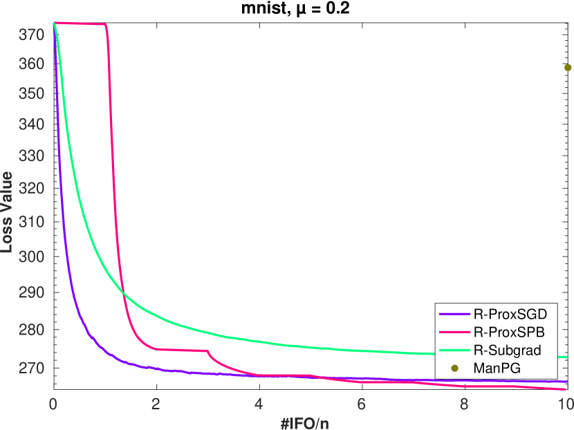
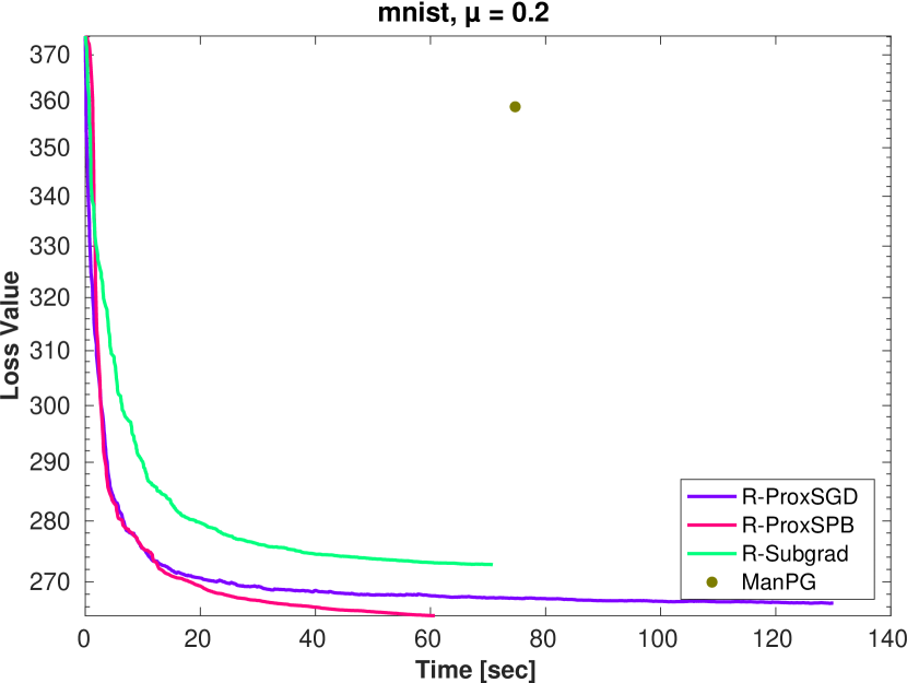
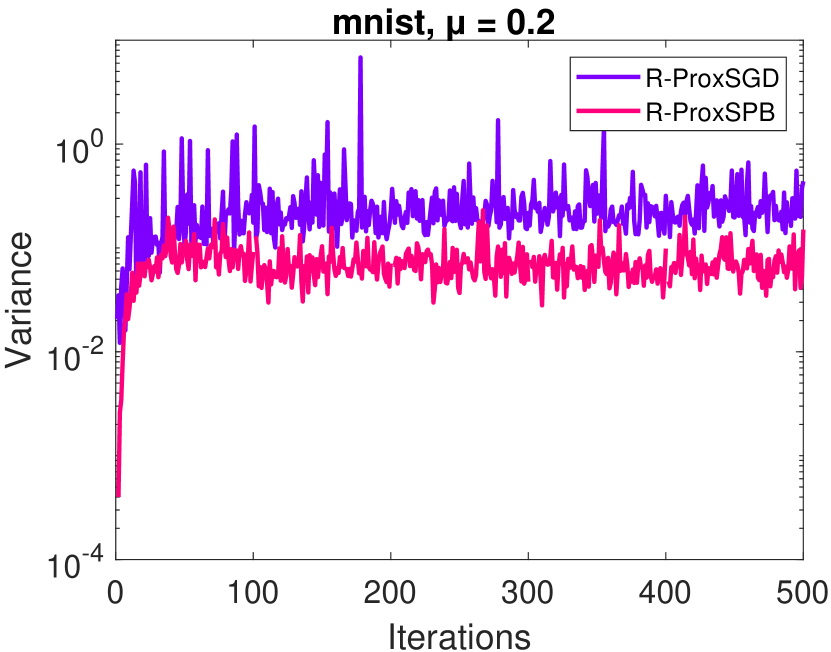
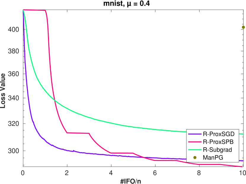
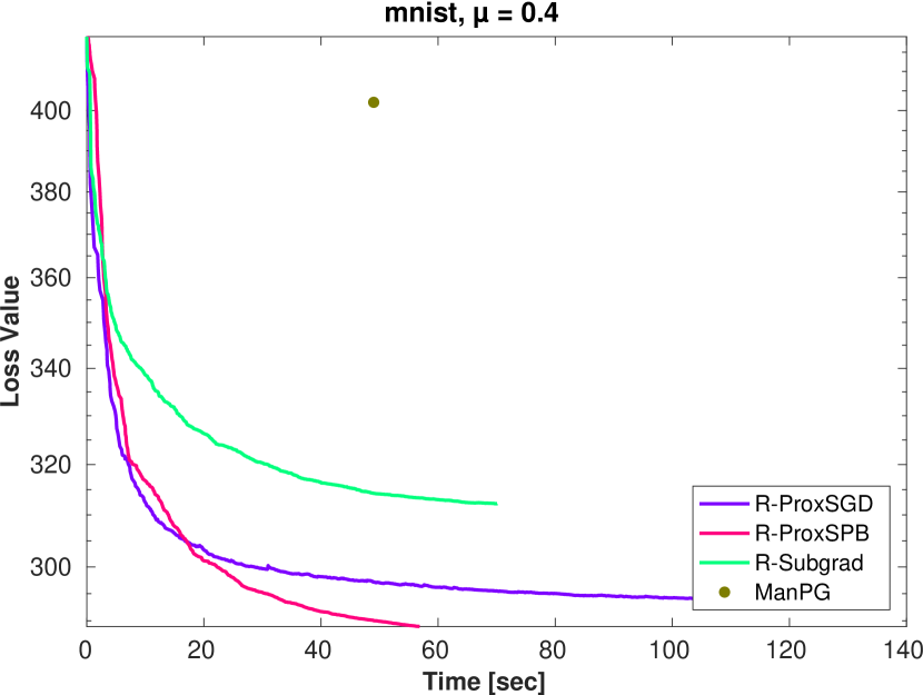
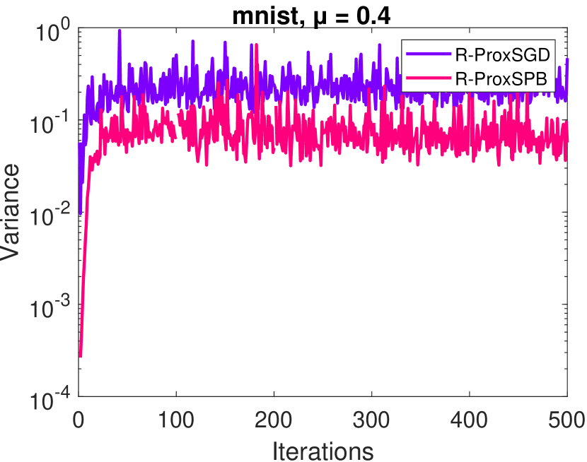
Figure 1: Experimental results on the mnist dataset with $\mu=0.2$ and $0.4$.

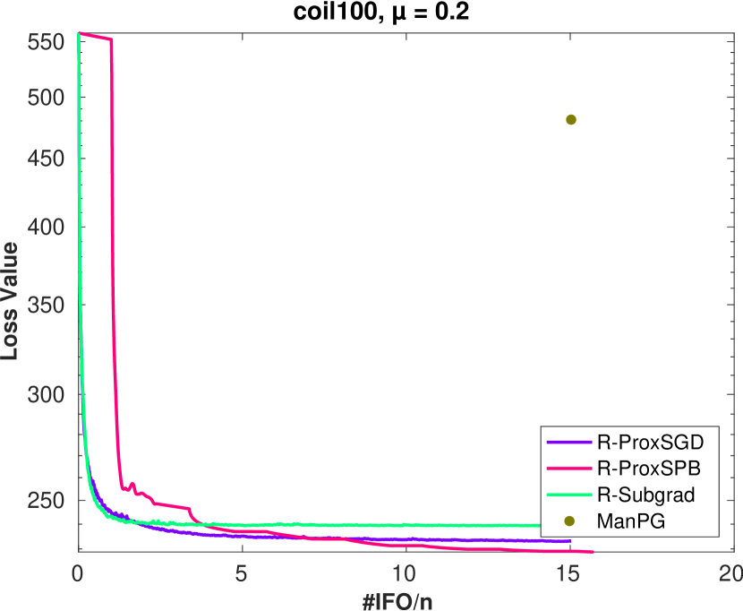
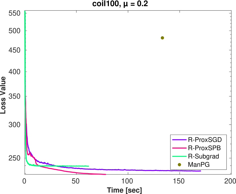
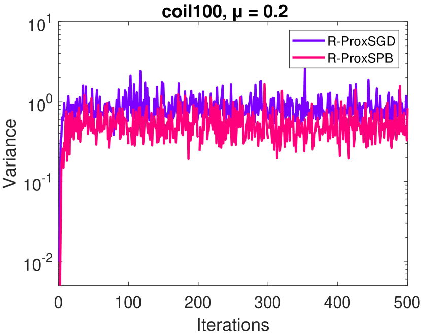
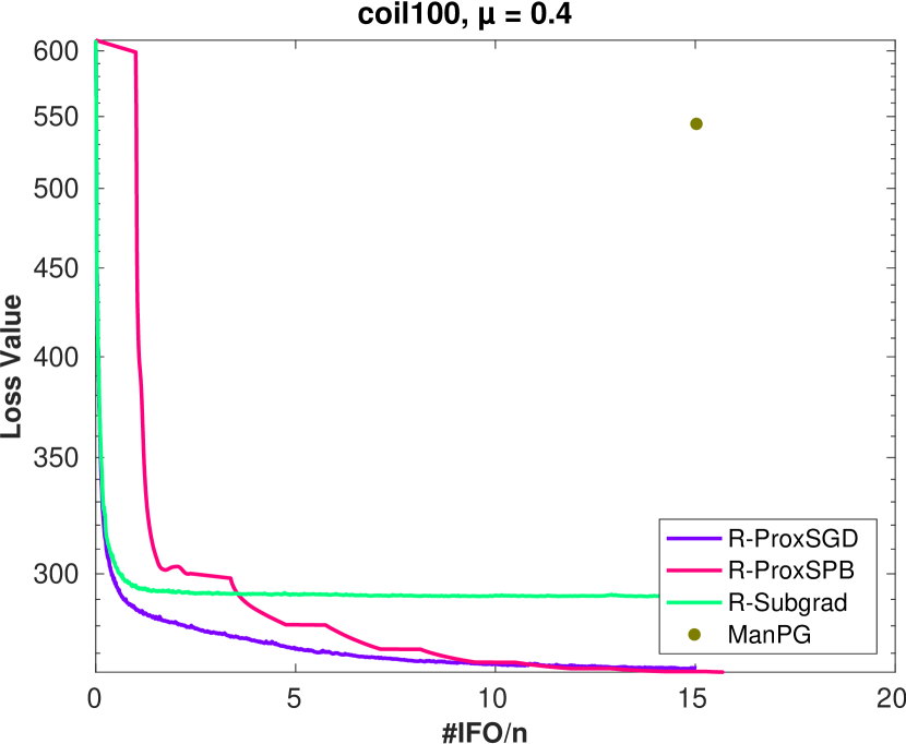
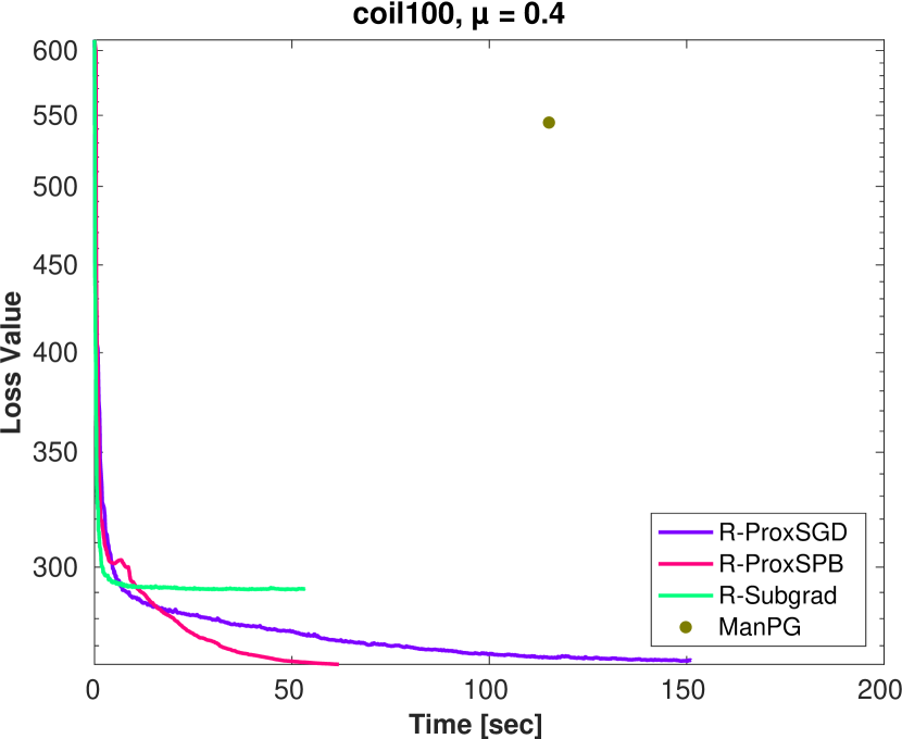
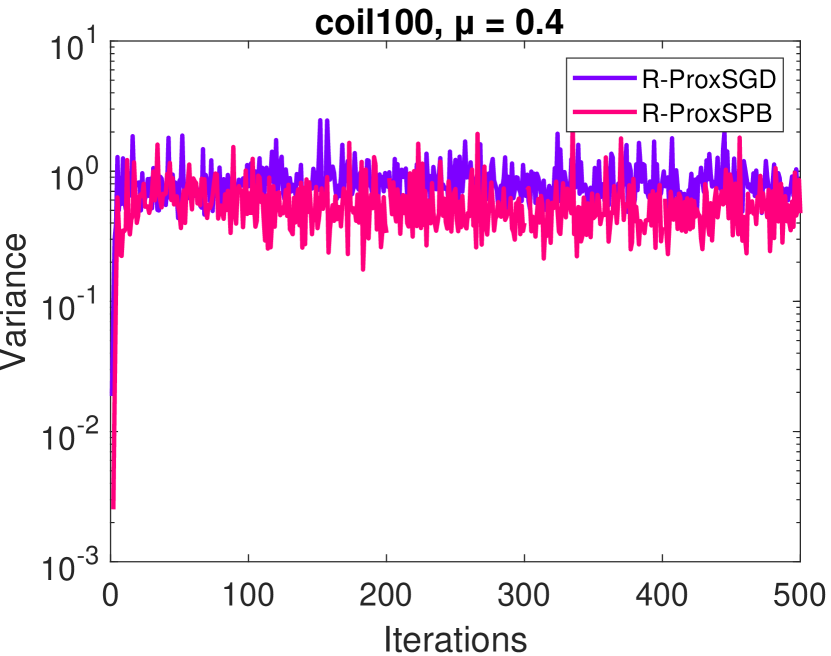
Figure 2: Experimental results on the coil100 dataset with $\mu=0.2$ and $0.4$.

All the results in Figures 1 and 2 indicate that both R-ProxSGD and R-ProxSPB consistently outperform R-Subgrad in terms of CPU time and the number of IFO calls. Moreover, these figures show that R-Subgrad is not able to reduce the loss value to a desired accuracy, comparing with R-ProxSGD and R-ProxSPB. Furthermore, these results also show that R-ProxSPB usually performs better than R-ProxSGD, which is consistent with our theoretical results on the complexity bounds. Figures 1 and 2 also imply that R-ProxSPB is effective to reduce the variance of the stochastic gradient on both datasets. We perform grid search to tune $\eta_{0}$ (used in R-Subgrad and R-ProxSGD) and $\eta$ (used in R-ProxSPB) from $\{5\times 10^{-5},10^{-4},5\times 10^{-4},...,1\}$. The best $\eta_{0}$ and $\eta$ on different data sets are reported in Table 3.

Figure 3 gives more results on the case $r=15$ and $\mu=0.2$, $0.4$, $0.8$, and here we only present the loss value versus the CPU time. These results further justify the advantages of our proposed R-ProxSGD and R-ProxSPB algorithms.

mnist data set				coil data set
$\mu$	R-Subgrad	R-ProxSGD	R-ProxSPB	$\mu$	R-Subgrad	R-ProxSGD	R-ProxSPB
0.2	0.01	0.005	0.005	0.2	0.005	0.01	0.005
0.4	0.01	0.01	0.005	0.4	0.01	0.01	0.005

Table 3: Chosen $\eta_{0}$ (for R-Subgrad and R-ProxSGD) and $\eta$ (for R-ProxSPB) for the reported results on mnist and coil data sets.

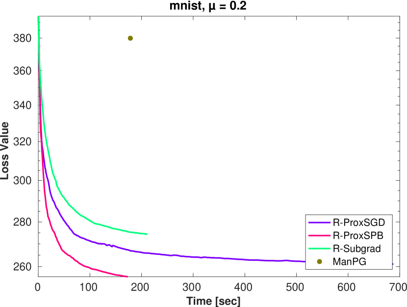
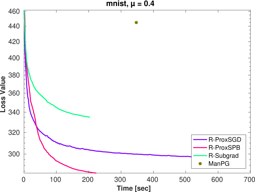
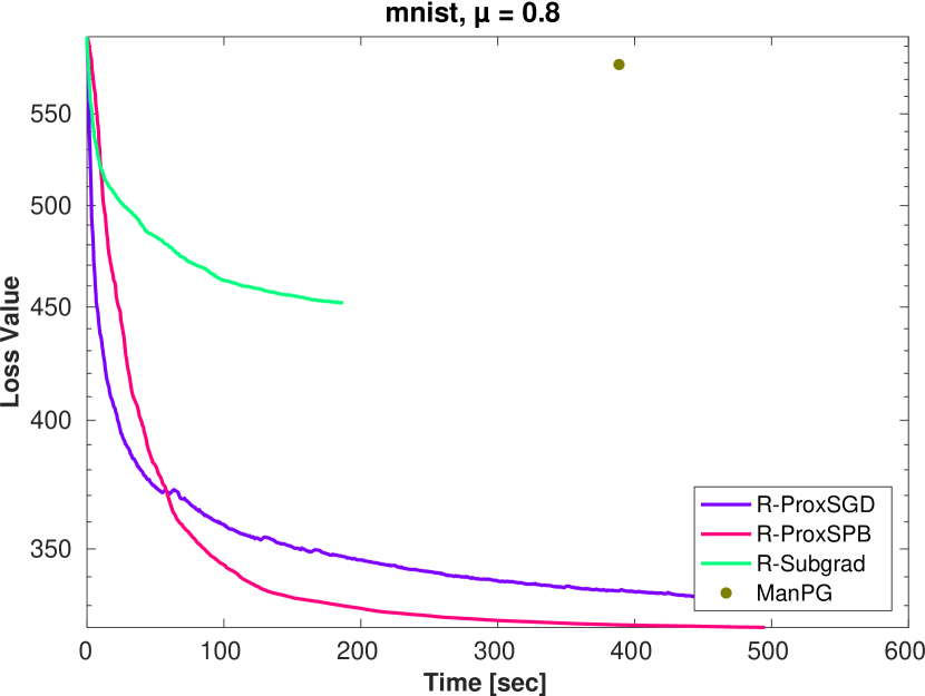
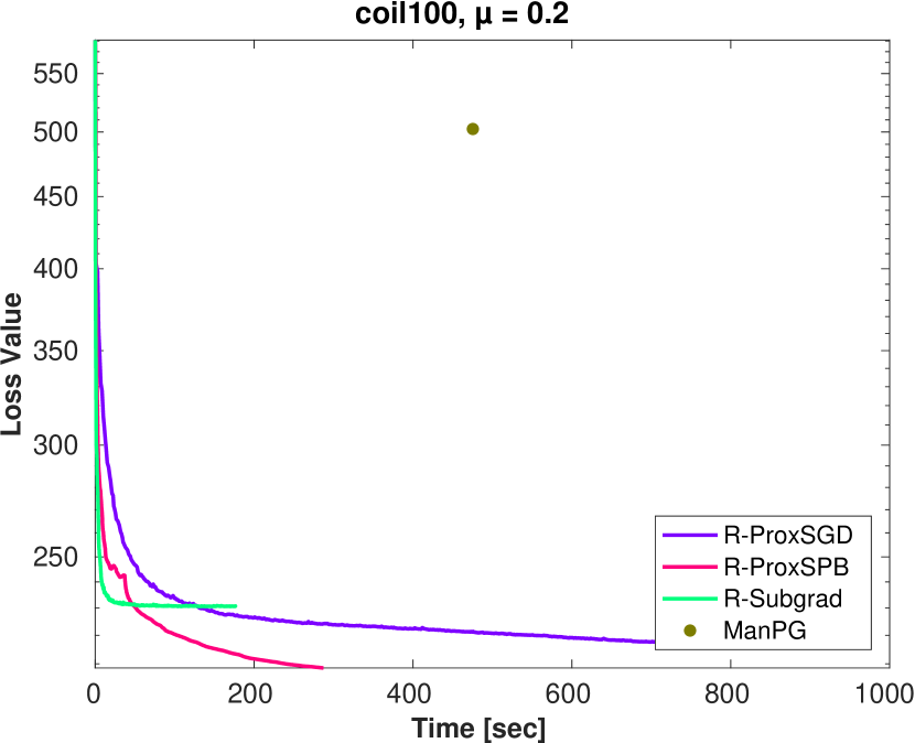
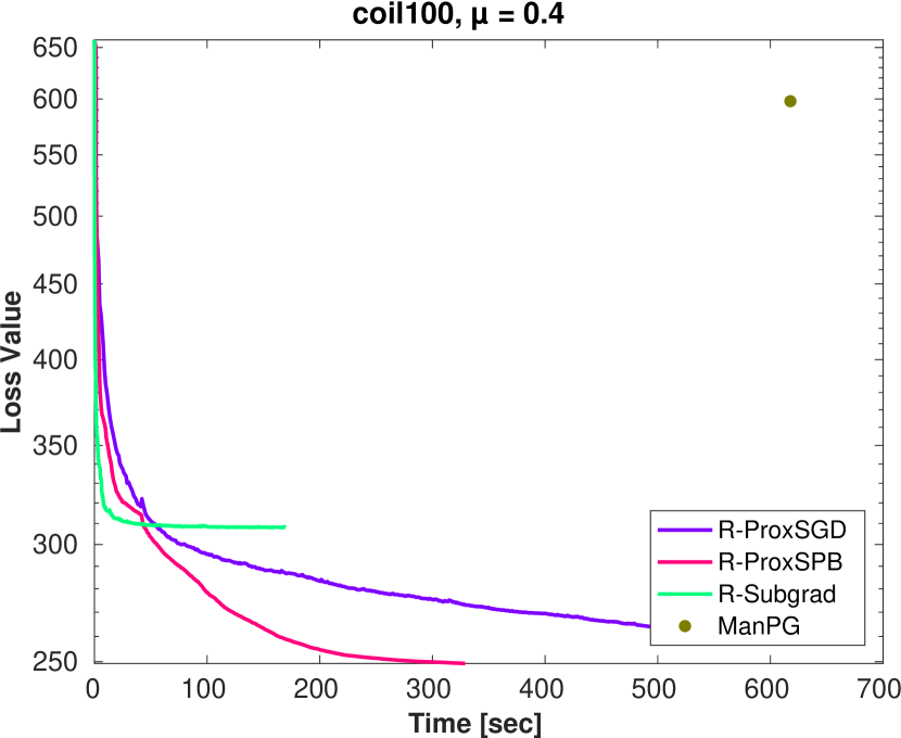
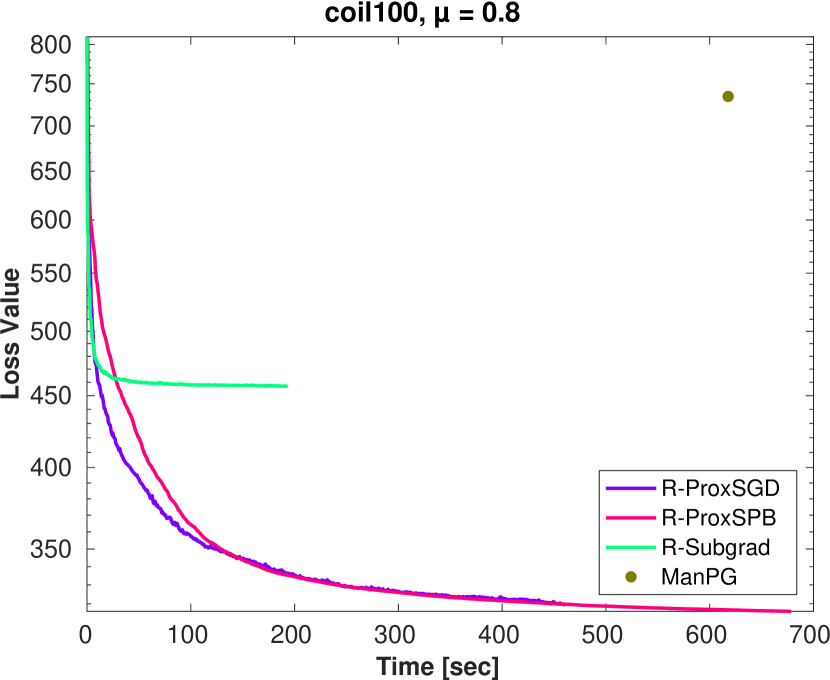
Figure 3: Loss value versus runtime on two datasets with $r=15$ and $\mu=0.2,0.4,0.8$.

4.1.2 Comparison with ManPG and SPAMS

To justify the necessity of introducing the stochasticity, we compare our R-ProxSGD and R-ProxSPB with the deterministic algorithm ManPG (Chen et al., 2020b), which also solves the same problem in (4) but assumes that the full gradient information for the smooth part is available. As shown in Figures 1 and 2, ManPG leads to larger loss values than our R-ProxSGD and R-ProxSPB given the same budget of gradient oracles or running time. We also point out that if the problem is online, then ManPG is not applicable.

Moreover, we also compare our R-ProxSPB algorithm with the SPAMS algorithm (Mairal et al., 2010) for the online sparse PCA problem. We run R-ProxSPB for 1000 iterations with batch size 100. For fair comparison, we run SPAMS using the same batch size and the same number of gradient oracles. Since the problem formulation of online sparse PCA in SPAMS is different from (4), we cannot directly compare the objective function value. Instead, we consider the explained variance and sparsity metrics as suggested in Yang and Xu (2015). The explained variance is defined as $\frac{\text{tr}(X^{\top}AA^{\top}X)}{\text{tr}(XX^{\top})}$, where $A\in\mathbb{R}^{d\times n}$ is the data matrix and $X\in\mathbb{R}^{d\times r}$ is the model parameter. The sparsity is defined as the number of elements in $X$ whose absolute value is larger than the threshold 0.001. As shown in Table 4, our R-ProxSPB leads to better sparsity while achieving comparable explained variance.

coil100 Data Set			mnist Data Set
Algorithms	Explained Variance	Sparsity	Algorithms	Explained Variance	Sparsity
SPAMS	0.0132	240	SPAMS	0.0179	185
R-ProxSPB	0.0120	22	R-ProxSPB	0.0190	18

Table 4: Comparison of R-ProxSPB and SPAMS (Mairal et al., 2010).

4.2 Robust Low-Rank Matrix Completion

Robust low-rank matrix completion is closely related to the robust PCA problem. The robust PCA aims to decompose a given matrix $M\in\mathbb{R}^{m\times n}$ into the superposition of a low-rank matrix $L$ and a sparse matrix $S$. Robust low-rank matrix completion is the same as robust PCA, except that only a subset of the entries of $M$ is observed. The convex formulations of them are studied extensively in the literature and we refer the reader to the recent survey (Ma and Aybat, 2018). A typical convex formulation of robust low-rank matrix completion is given as follows:

$$\min_{L,S}\ \|L\|_{*}+\gamma\|S\|_{1},\ \textrm{s.t.},\ \mathcal{P}_{\Omega}(L+S)=\mathcal{P}_{\Omega}(M),$$ (21)

where $\|L\|_{*}$ denotes the nuclear norm of $L$ and it sums the singular values of $L$, $\Omega$ is a subset of the index set $\{(i,j)\mid 1\leq i\leq m,1\leq j\leq n\}$, and the projection operator $\mathcal{P}_{\Omega}$ is defined as: $[\mathcal{P}_{\Omega}(Z)]_{ij}=Z_{ij}$, if $(i,j)\in\Omega$, and $[\mathcal{P}_{\Omega}(Z)]_{ij}=0$ otherwise. Due to the presence of the nuclear norm in (21), algorithms for solving (21) usually require computing the SVD of an $m\times n$ matrix in every iteration, which can be time consuming when $m$ and $n$ are large. Recently, some nonconvex formulations of robust low-rank matrix completion were proposed because they allow more efficient and scalable algorithms. In Huang et al. (2020), the authors proposed the following nonconvex formulation of robust low-rank matrix completion:

$$\min_{\mathbb{U}\in\mathrm{Gr}(m,r),V\in\mathbb{R}^{r\times n},S\in\mathbb{R}^{m\times n}}\frac{1}{2}\|\mathcal{P}_{\Omega}(UV-M+S)\|^{2}_{F}+\frac{\lambda}{2}\|\mathcal{P}_{\bar{\Omega}}(UV)\|^{2}_{F}+\gamma\|\mathcal{P}_{\Omega}(S)\|_{1},$$ (22)

where $\mathrm{Gr}(m,r)$ denotes the Grassmann manifold, which is the set of $r$-dimensional vector subspaces of $\mathbb{R}^{m}$, and we use $U\in\mathbb{R}^{m\times r}$ to denote a basis of the subspace $\mathbb{U}\in\mathrm{Gr}(m,r)$. In (22), the low-rank matrix $L$ is replaced by $UV$ with $U\in\mathbb{R}^{m\times r}$, $V\in\mathbb{R}^{r\times n}$, and $r$ is the estimation of the rank of $L$; the term $\frac{\lambda}{2}\|\mathcal{P}_{\bar{\Omega}}(UV)\|^{2}_{F}$ is added as a regularizer and $\lambda>0$ is sufficiently small indicating that we have a small confidence of the components of $UV$ on $\bar{\Omega}$ being zeros; the constraint $\mathbb{U}\in\mathrm{Gr}(m,r)$ is added to remove the scaling ambiguity of $U$ and $V$. The nonconvex formulation (22) was motivated by some recent works on Riemannian optimization (Boumal and Absil, 2011; Cambier and Absil, 2016). Note that, for fixed $U$ and $S$, the variable $V$ in (22) can be uniquely determined. By denoting

$$\bar{f}(U,V,S)=\frac{1}{2}\|\mathcal{P}_{\Omega}(UV-M+S)\|_{F}^{2}+\frac{\lambda}{2}\|\mathcal{P}_{\bar{\Omega}}(UV)\|_{F}^{2},$$ (23)

and

$$V_{U,S}:=\mathop{\mathrm{argmin}}_{V}\ \bar{f}(U,V,S),\mbox{ and }f(U,S)=\bar{f}(U,V_{U,S},S),$$ (24)

we can rewrite (22) as

$$\min_{\mathbb{U}\in\mathrm{Gr}(m,r),S\in\mathbb{R}^{m\times n}}f(U,S)+\gamma\|\mathcal{P}_{\Omega}(S)\|_{1},$$ (25)

which is a Riemannian optimization problem with nonsmooth objective. Note that although the manifold is the Grassmann manifold instead of the Stiefel manifold, our algorithms discussed in Section 3 can be directly applied to (25). To see this, first note that as suggested in (Boumal and Absil, 2011), without loss of generality, we can restrict matrix $U$ as an orthonormal basis of $\mathbb{U}$. Therefore, we have

$$\|\mathcal{P}_{\bar{\Omega}}(UV)\|_{F}^{2}=\|UV\|_{F}^{2}-\|\mathcal{P}_{\Omega}\|_{F}^{2}=\|V\|_{F}^{2}-\|\mathcal{P}_{\Omega}\|_{F}^{2},$$

and thus we can rewrite $\bar{f}(U,V,S)$ and $f(U,S)$ as

$$\bar{f}(U,V,S)=\frac{1}{2}\|\mathcal{P}_{\Omega}(UV-M+S)\|_{F}^{2}+\frac{\lambda}{2}\|V\|^{2}_{F}-\frac{\lambda}{2}\|\mathcal{P}_{\Omega}(UV)\|_{F}^{2}.$$ (26)

$$f(U,S)=\frac{1}{2}\|\mathcal{P}_{\Omega}(UV_{U,S}-M+S)\|_{F}^{2}+\frac{\lambda}{2}\|V_{U,S}\|^{2}_{F}-\frac{\lambda}{2}\|\mathcal{P}_{\Omega}(UV_{U,S})\|_{F}^{2}.$$ (27)

From (24) we know that $\nabla_{V}\bar{f}(U,V_{U,S},S)=0$. Therefore,

$$\nabla_{U}f(U,S)=\nabla_{U}\bar{f}(U,V_{U,S},S)=\nabla_{1}\hat{f}(U,V_{U,S},S),$$

where

$$\hat{f}(U,V_{U,S},S):=\frac{1}{2}\|\mathcal{P}_{\Omega}(UV_{U,S}-M+S)\|_{F}^{2}-\frac{\lambda}{2}\|\mathcal{P}_{\Omega}(UV_{U,S})\|_{F}^{2}=\sum_{(i,j)\in\Omega}\hat{f}_{ij}(U,V_{U,S},S),$$ (28)

and

$$\hat{f}_{ij}(U,V_{U,S},S)=\frac{1}{2}(UV_{U,S}-M+S)_{ij}^{2}-\frac{\lambda}{2}(UV_{U,S})_{ij}^{2}.$$

That is, $\hat{f}$ in (28) has a natural finite-sum structure, and a stochastic gradient approximation to $\nabla_{U}f(U,S)$ is given by $\nabla_{1}\hat{f}_{ij}(U,V_{U,S},S)$ with randomly sampled index pair $(i,j)\in\Omega$. It is easy to verify that

$$\nabla_{1}\hat{f}_{ij}(U,V_{U,S},S)=(u_{i}^{\top}v_{j}-M_{ij}+S_{ij}-\lambda u_{i}^{\top}v_{j})\bar{V}_{j}^{\top},$$

where $u_{i}^{\top}$ denotes the $i$-th row of $U$, and $v_{j}$ denotes the $j$-th column of $V_{U,S}$, and

$$\bar{V}_{j}=\begin{bmatrix}0&0&\cdots&v_{j}&\cdots&0\end{bmatrix}.$$

That is, $\bar{V}_{j}\in\mathbb{R}^{r\times m}$ is a matrix whose $j$-th column is $v_{j}$ and all other columns are zeros. Clearly, when computing $\nabla_{U}f_{ij}(U,S)$, we only need to access $u_{i}^{\top}$ and $v_{j}$ and we do not need to access the whole matrix $U$ and $V_{U,S}$ and compute the matrix multiplication $UV_{U,S}$, and this is very useful when $m$ and $n$ are large.

We applied our R-ProxSGD and R-ProxSPB algorithms to solve the robust low-rank matrix completion problem (25) on some real data for video background estimation (Li et al., 2004) and we again compared their performance with R-Subgrad. We consider two surveillance video datasets: “Hall of a business building” and “Airport elevator”. The data matrix $X^{*}$ is obtained by vectorizing each grayscale frame of the video. We then randomly sample 50% of the indices to obtain $\Omega$, and then sample the entries of $X^{*}$ from $\Omega$ to get $M$. A sparse matrix $S^{*}$ was then added to $M$. In R-ProxSGD and R-Subgrad, we randomly sample 10% of the known entries as a batch in each iteration. In R-ProxSPB, we set $|\mathcal{S}_{t}^{1}|=|\Omega|$ and $q=5$. The initial step sizes $\eta_{0}$ are tuned from $\{10^{-j}/|\Omega|,~{}i=0,1,\ldots,4\}$.

In Figure 4, we present the experimental results on the problem with those two real datasets. For fair comparison, we report the results of all algorithms using the same budget of stochastic gradients, which is $4|\Omega|$. The results in Figure 4 clearly show the advantage of our R-ProxSPB and R-ProxSGD algorithms over R-Subgrad algorithm.

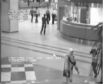
(a) Original Image

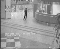
(b) R-ProxSPB
time=2.58

(c) R-ProxSGD
time=5.76

(d) R-Subgrad
time=2.26

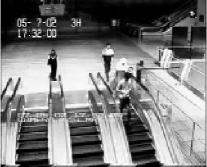
(e) Original Image

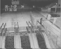
(f) R-ProxSPB
time=3.11

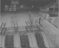
(g) R-ProxSGD
time=6.99

(h) R-Subgrad
time=2.45

Figure 4: First row: background estimation from partial observations on the “Hall of a business building” data set; Second row: background estimation from partial observations on the “Airport elevator” data set.

5 Conclusion

In this paper, we considered the nonsmooth Riemannian optimization problems with nonsmooth regularizer in the objective. We designed Riemannian stochastic algorithms that do not need subgradiet information for solving this class of problems. Specifically, we proposed two Riemannian stochastic proximal gradient algorithms: R-ProxSGD and R-ProxSPB to solve this problem. The two proposed algorithms are generalizations of their counterparts in Euclidean space to Riemannian manifold setting. We analyzed the iteration complexity and IFO complexity of the proposed algorithms for obtaining an $\epsilon$-stationary point. Numerical results on solving online sparse PCA and robust low-rank matrix completion are conducted which demonstrate that our proposed algorithms outperform significantly the Riemannian stochastic subgradient method. Future work includes extending the current results to more general Riemannian manifolds.

A Auxiliary Definitions and Lemmas

In this section we give a few lemmas and definitions that are necessary to our analysis. These lemmas are proved in existing works, so we do not include the proof here.

Definition 17 (Generalized Clarke subdifferential, see Hosseini and Pouryayevali (2011))

For a locally Lipschitz function $F$ on the manifold $\mathcal{M}$, the Riemannian generalized directional derivative $F^{\circ}(X,\zeta)$ at $X\in\mathcal{M}$ in the direction $\zeta$ is defined by

$$\limsup\limits_{Y\rightarrow X,t\downarrow 0}\frac{F\circ\phi^{-1}(\phi(Y)+tD\phi(X)[\zeta])-f\circ\phi^{-1}(\phi(Y))}{t}.$$

Here $(\phi,U)$ is a coordinate chart at $X$. The Clarke subdifferential $\hat{\partial}F(X)$ at $X\in\mathcal{M}$ is:

$$\hat{\partial}F(X)=\{\xi\in\mathrm{T}_{X}\mathcal{M}:\langle\xi,V\rangle\leq F^{\circ}(X,\zeta),\forall\zeta\in\mathrm{T}_{X}\mathcal{M}\}.$$

Lemma 18

Suppose $g_{i}$ is the unbiased and variance-bounded stochastic estimator of $g$ on randomly sampled instance $i$, i.e. $\mathbb{E}_{i}[g_{i}]=g$ and $\mathbb{E}_{i}[\|g_{i}-g\|^{2}]\leq\sigma^{2}$. Then we can conclude that the estimator $g_{\mathcal{S}}:=\frac{1}{|\mathcal{S}|}\sum_{i\in\mathcal{S}}g_{i}$ based on randomly sampled mini-batch $\mathcal{S}$ is also unbiased and variance-bounded:

$$\mathbb{E}_{\mathcal{S}}[g_{\mathcal{S}}]=g,\quad\mathbb{E}_{\mathcal{S}}[\|g_{\mathcal{S}}-g\|^{2}]\leq\frac{\sigma^{2}}{|\mathcal{S}|}.$$ (29)

The following lemmas from previous works (Absil et al., 2009; Kasai et al., 2018; Zhou et al., 2019) under Assumptions 4-8 regarding retraction and vector transport are very useful.

Lemma 19 (Retraction $L_{R}$ smoothness, Lemma 3.5 in Kasai et al. (2018))

If $f(X)$ has an upper-bounded Hessian, there exists a neighborhood $\mathcal{U}$ of any $X\in\mathcal{M}$ and a constant $L_{R}>0$ such that $\forall X,Y\in\mathcal{U},\textrm{Retr}_{X}(\xi)=Y,\xi\in\mathrm{T}_{X}\mathcal{M}$:

$$f(Y)\leq f(X)+\langle\nabla f(X),\xi\rangle+\frac{L_{R}}{2}\|\xi\|^{2}.$$ (30)

Lemma 20 (Lemma 3.7 in Kasai et al. (2018))

Under Assumption 4(ii), there exists a constant $\theta>0$, such that the following inequalities hold for any $X,Y\in\mathcal{U}$:

$$\|\Gamma_{\eta}\xi-P_{\eta}\xi\|\leq\theta\|\xi\|_{X}\|\eta\|_{X},\quad\|\Gamma^{-1}_{\eta}\xi-P^{-1}_{\eta}\xi\|\leq\theta\|\chi\|_{X}\|\eta\|_{X},$$

where $\xi,\eta\in\mathrm{T}_{X}\mathcal{M}$, $\chi\in\mathrm{T}_{Y}\mathcal{M}$, $\textrm{Retr}_{X}(\eta)=Y$.

Lemma 21 (Lemma 4 in Zhou et al. (2019))

Given $\hat{X}\in\mathcal{M}$ that does not depend on the update sequence $\{X_{t}\}$, the following inequality about the retraction and vector transport holds:

$$\mathbb{E}_{i}[\|\Gamma_{X_{t}}^{\hat{X}}(\nabla f_{i}(X_{t}))-\Gamma_{X_{t-1}}^{\hat{X}}\nabla f_{i}(X_{t-1})\|^{2}]\leq 2\Theta^{2}\|\textrm{Retr}_{X_{t-1}}^{-1}(X_{t})\|^{2},$$ (31)

where $\Theta^{2}=\theta^{2}G^{2}+2(1+c_{R})L_{H}^{2}$ and $\theta$ is defined in Lemma 20.

Lemma 22 (Lemma 1 in Zhou et al. (2019))

Let $n_{t}=\lceil t/q\rceil$, $(n_{t}-1)q\leq t\leq n_{t}q$, $t_{0}=(n_{t}-1)q$, where $\lceil a\rceil$ denotes the smallest integer that is larger than $a$. Mini-batches $\mathcal{S}^{1}_{t}$, $\mathcal{S}_{t}^{2}$ are selected as described in Algorithm 2. Under the Assumptions 4-8, the estimation error between the R-SARAH estimator $V_{t}$ generated by Algorithm 2 and full gradient $\nabla f(X_{t})$ is bounded by:

$$\mathbb{E}[\|V_{t}-\nabla f(X_{t})\|^{2}]\leq I\{|\mathcal{S}_{t}^{1}|<n\}\cdot\frac{\sigma^{2}}{|\mathcal{S}_{t}^{1}|}+\sum_{i=t_{0}}^{t-1}\frac{\Theta^{2}}{|\mathcal{S}_{t}^{2}|}\mathbb{E}[\|\textrm{Retr}_{X_{i}}^{-1}(X_{i+1})\|^{2}],$$

where $I\{\cdot\}$ denotes an indicator function.

For the ease of presentation, we adopt the following notation, which is consistent with the ones used in (11) and (15).

$$\zeta_{t} :=\mathop{\mathrm{argmin}}_{\zeta\in\mathrm{T}_{X_{t}}\mathcal{M}}\{\phi_{t}(\zeta):=\langle V_{t},\zeta\rangle+\frac{1}{2\gamma}\|\zeta\|^{2}+h(X_{t}+\zeta)\},$$ (32)

$$\xi_{t} :=\mathop{\mathrm{argmin}}_{\xi\in\mathrm{T}_{X_{t}}\mathcal{M}}\{\langle\nabla f(X_{t}),\xi\rangle+\frac{1}{2\gamma}\|\xi\|^{2}+h(X_{t}+\xi)\}.$$ (33)

Moreover, note that according to the definition of $\mathcal{F}_{t}$, when we take conditional expectation $\mathbb{E}[\cdot\mid\mathcal{F}_{t-1}]$, $X_{t}$ in both R-ProxSGD and R-ProxSPB has been realized.

B Necessary Lemmas for Proving Theorem 13

Lemma 23

The solution $\mathbf{\zeta}_{t}$ defined in (32) satisfies:

$$\mathbb{E}[\phi_{t}(\eta_{t}\mathbf{\zeta}_{t})|\mathcal{F}_{t-1}]-\phi_{t}(0)\leq\frac{(\eta_{t}-2)\eta_{t}}{2\gamma}\mathbb{E}[\|\mathbf{\zeta}_{t}\|^{2}|\mathcal{F}_{t-1}].$$ (34)

Proof Note that $\phi_{t}(\mathbf{\zeta})$ is $(1/\gamma)$-strongly convex with respect to $\mathbf{\zeta}$. For $\mathbf{\zeta}_{1},\mathbf{\zeta}_{2}\in\mathrm{T}_{X_{t}}\mathcal{M}$, we have:

$$\phi_{t}(\mathbf{\zeta}_{2})\geq\phi_{t}(\mathbf{\zeta}_{1})+\langle\hat{\partial}\phi_{t}(\mathbf{\zeta}_{1}),\mathbf{\zeta}_{2}-\mathbf{\zeta}_{1}\rangle+\frac{1}{2\gamma}\|\mathbf{\zeta}_{2}-\mathbf{\zeta}_{1}\|^{2}.$$ (35)

Note that the optimality conditions of (32) are given by $0\in\mathrm{Proj}_{\mathrm{T}_{X_{t}}\mathcal{M}}\partial\phi_{t}(\mathbf{\zeta}_{t})$. Therefore,

$$\langle\hat{\partial}\phi_{t}(\mathbf{\zeta}_{1}),\mathbf{\zeta}_{2}-\mathbf{\zeta}_{1}\rangle=\langle\mathrm{Proj}_{\mathrm{T}_{X_{t}}\mathcal{M}}\partial\phi_{t}(\mathbf{\zeta}_{1}),\mathbf{\zeta}_{2}-\mathbf{\zeta}_{1}\rangle=0,\forall\mathbf{\zeta}_{1},\mathbf{\zeta}_{2}\in\mathrm{T}_{X_{t}}\mathcal{M}.$$ (36)

Letting $\mathbf{\zeta}_{1}=\mathbf{\zeta}_{t}$ and $\mathbf{\zeta}_{2}=0$ in (35), and combining with (36), we have

$$\phi_{t}(0)\geq\phi_{t}(\mathbf{\zeta}_{t})+\frac{1}{2\gamma}\|\mathbf{\zeta}_{t}\|^{2},$$

which is equivalent to:

$$h(X_{t}+\mathbf{\zeta}_{t})-h(X_{t})\leq\langle-V_{t},\mathbf{\zeta}_{t}\rangle-\frac{1}{\gamma}\|\mathbf{\zeta}_{t}\|^{2}.$$ (37)

According to the definition of $\phi_{t}$, $\phi_{t}(\eta_{t}\mathbf{\zeta}_{t})-\phi_{t}(0)$ can be written as:

$$\phi_{t}(\eta_{t}\mathbf{\zeta}_{t})-\phi_{t}(0)=\eta_{t}\langle V_{t},\mathbf{\zeta}_{t}\rangle+\frac{\eta_{t}^{2}}{2\gamma}\|\mathbf{\zeta}_{t}\|^{2}+h(X_{t}+\eta_{t}\mathbf{\zeta}_{t})-h(X_{t}).$$ (38)

From (37) and the convexity of $h$: $h(X_{t}+\eta_{t}\mathbf{\zeta}_{t})\leq\eta_{t}h(X_{t}+\mathbf{\zeta}_{t})+(1-\eta_{t})h(X_{t})$, $\eta_{t}\in(0,1]$, we have

$$h(X_{t}+\eta_{t}\mathbf{\zeta}_{t})-h(X_{t})\leq-\eta_{t}\langle V_{t},\mathbf{\zeta}_{t}\rangle-\frac{\eta_{t}}{\gamma}\|\mathbf{\zeta}_{t}\|^{2}.$$ (39)

Combine (38) and (39) and take expectation conditioned on $\mathcal{F}_{t-1}$ on both sides, we get the desired result.  

The following lemma justifies why $G(X,\nabla f(X),\gamma)$ is valid for defining the $\epsilon$-stationary solution.

Lemma 24

If $G(X,\nabla f(X),\gamma)=0$, and the retraction is given by the Polar decomposition: $\textrm{Retr}_{X}(\xi)=(X+\xi)(I+\xi^{\top}\xi)^{-\frac{1}{2}}$, then $X$ is a stationary point of problems (1), i.e., $0\in\nabla f(X)+\mathrm{Proj}_{\mathrm{T}_{X}\mathcal{M}}\partial h(X)$.

To prove Lemma 24, we first need to show the following Lemma.

Lemma 25

Consider $X\in\mathcal{M}$, $\mathcal{M}$ is the Stiefel manifold and $\xi\in T_{X}\mathcal{M}$. If $X=\textrm{Retr}_{X}(\xi)$, where the retraction is given by the Polar decomposition: $\textrm{Retr}_{X}(\xi)=(X+\xi)(I+\xi^{\top}\xi)^{-\frac{1}{2}}$, then $\xi=\mathbf{0}_{X}$.

Proof If $X=\textrm{Retr}_{X}(\xi)=(X+\xi)(I+\xi^{\top}\xi)^{-\frac{1}{2}}$, then we have

$$X+\xi=X(I+\xi^{\top}\xi)^{\frac{1}{2}}.$$ (40)

Since $X^{\top}X=I$, (40) leads to

$$X^{\top}X+\xi^{\top}X=(I+\xi^{\top}\xi)^{\frac{1}{2}}$$ (41)

and

$$X^{\top}X+X^{\top}\xi=(I+\xi^{\top}\xi)^{\frac{1}{2}}.$$ (42)

Since $\xi\in\mathrm{T}_{X}\mathcal{M}$, we have $\xi^{\top}X+X^{\top}\xi=0$. Adding (41) and (42) gives $2I=2(I+\xi^{\top}\xi)^{\frac{1}{2}}$, which implies $\xi=\mathbf{0}_{X}$.  

Now we are ready to give the proof of Lemma 24.

Proof If $G(X_{t},\nabla f(X_{t}),\gamma)=0$, we have $\xi_{t}=\mathbf{0}_{X_{t}}$ because of Lemma 25. According to Yang et al. (2014), the optimality conditions of (33) are given by

$$0\in\nabla f(X_{t})+\frac{1}{\gamma}\xi_{t}+\mathrm{Proj}_{\mathrm{T}_{X_{t}}\mathcal{M}}\partial h(X_{t}+\xi_{t}).$$

Thus, $G(X_{t},\nabla f(X_{t}),\gamma)=0$ leads to that $0\in\nabla f(X_{t})+\mathrm{Proj}_{\mathrm{T}_{X_{t}}\mathcal{M}}\partial h(X_{t})$, which means $X_{t}$ is a stationary point of problem (1).  

The following lemma shows the progress of the algorithm in one iteration in terms of objective function value.

Lemma 26

Denote $X_{t}^{+}:=X_{t}+\eta_{t}\mathbf{\zeta}_{t}$. The following inequality holds:

$$F(X_{t+1})\!-\!F(X_{t})\!\leq\!\frac{(L_{R}\gamma-1)\eta_{t}^{2}}{2\gamma}\|\mathbf{\zeta}_{t}\|^{2}\!+\!h(X_{t+1})\!-\!h(X_{t}^{+})+\phi_{t}(\eta_{t}\mathbf{\zeta}_{t})-\phi_{t}(0)+\eta_{t}\langle\nabla f(X_{t})-V_{t},\mathbf{\zeta}_{t}\rangle.$$

Proof Consider the update $X_{t+1}=\textrm{Retr}_{X_{t}}(\eta_{t}\zeta_{t})$. By applying Lemma 19 with $X=X_{t},Y=X_{t+1}$ and $\xi=\eta_{t}\zeta_{t}$, we get

$$f(X_{t+1})-f(X_{t})\leq\eta_{t}\langle\nabla f(X_{t}),\zeta_{t}\rangle+\frac{L_{R}\eta_{t}^{2}}{2}\|\zeta_{t}\|^{2},$$

which leads to:

$$F(X_{t+1})-F(X_{t})\leq\frac{L_{R}\eta_{t}^{2}}{2}\|\mathbf{\zeta}_{t}\|^{2}+\eta_{t}\langle\nabla f(X_{t}),\mathbf{\zeta}_{t}\rangle+h(X_{t+1})-h(X_{t}).$$ (43)

Denote $X_{t}^{+}:=X_{t}+\eta_{t}\mathbf{\zeta}_{t}$. The definition of $\phi_{t}$ indicates:

$$\eta_{t}\langle V_{t},\mathbf{\zeta}_{t}\rangle=\phi_{t}(\eta_{t}\mathbf{\zeta}_{t})-\phi_{t}(0)-\frac{\eta_{t}^{2}}{2\gamma}\|\mathbf{\zeta}_{t}\|^{2}-h(X_{t}^{+})+h(X_{t}).$$ (44)

Combining (43) and (44) gives the desired result.  

The following lemma gives an upper bound to the size of $G(X_{t},\nabla f(X_{t}),\gamma)$.

Lemma 27

With $\zeta_{t}$ and $\xi_{t}$ defined in (32) and (33), for $G(X_{t},\nabla f(X_{t}),\gamma)=\frac{1}{\gamma}(X_{t}-\mathrm{Retr}_{X_{t}}(\xi_{t}))$, it holds that

$$\|G(X_{t},\nabla f(X_{t}),\gamma)\|^{2}\!\leq\!2M_{1}^{2}(7\|\zeta_{t}\|^{2}\!+\!4\gamma\|V_{t}\!-\!\nabla f(X_{t})\|^{2}).$$ (45)

Proof Let $G(X_{t},V_{t},\gamma)=\frac{1}{\gamma}(X_{t}-\mathrm{Retr}_{X_{t}}(\gamma\zeta_{t}))$. We first have the following trivial inequality:

$$\|G(X_{t},\nabla f(X_{t}),\gamma)\|^{2}\leq 2\|G(X_{t},V_{t},\gamma)\|^{2}+2\|G(X_{t},V_{t},\gamma)-G(X_{t},\nabla f(X_{t}),\gamma)\|^{2}.$$ (46)

The first term on the right hand side of (46) can be bounded based on the property of retraction in Assumption 4 (iii):

$$\|G(X_{t},V_{t},\gamma)\|^{2}=\frac{1}{\gamma^{2}}\|X_{t}-\mathrm{Retr}_{X_{t}}(\gamma\zeta_{t})\|^{2}\leq M_{1}^{2}\|\zeta_{t}\|^{2}.$$ (47)

The second term on the right hand side of (46) can be bounded as:

$$\|G(X_{t},V_{t},\gamma)-G(X_{t},\nabla f(X_{t}),\gamma)\|^{2}\leq\frac{2\|X_{t}-\mathrm{Retr}_{X_{t}}(\gamma\zeta_{t})\|^{2}}{\gamma^{2}}+\frac{2}{\gamma^{2}}\|X_{t}-\mathrm{Retr}_{X_{t}}(\gamma\xi_{t})\|^{2},$$ (48)

which further implies

$$\|G(X_{t},V_{t},\gamma)-G(X_{t},\nabla f(X_{t}),\gamma)\|^{2}\leq 2M_{1}^{2}(\|\zeta_{t}\|^{2}+\|\xi_{t}\|^{2})\leq 2M_{1}^{2}(3\|\zeta_{t}\|^{2}+2\|\xi_{t}-\zeta_{t}\|^{2}).$$ (49)

The optimality conditions of (32) and (33) are given by (see Yang et al. (2014)):

$$0\in V_{t}+\frac{1}{\gamma}\zeta_{t}+\mathrm{Proj}_{T_{X_{t}}\mathcal{M}}\partial h(X_{t}+\zeta_{t}),$$ (50)

$$0\in\nabla f(X_{t})+\frac{1}{\gamma}\xi_{t}+\mathrm{Proj}_{T_{X_{t}}\mathcal{M}}\partial h(X_{t}+\xi_{t}).$$ (51)

Let $X_{t}^{\dagger}=X_{t}+\xi_{t}$ and $X_{t}^{+}=X_{t}+\zeta_{t}$. (50) and (51) indicate that for any $\mathbf{u}\in\mathrm{T}_{X_{t}}\mathcal{M}$, there exist $p^{+}\in\partial h(X_{t}^{+})$ and $p^{\dagger}\in\partial h(X_{t}^{\dagger})$ such that

$$\langle\frac{1}{\gamma}\zeta_{t}+V_{t}+\mathrm{Proj}_{T_{X_{t}}\mathcal{M}}p^{+},\mathbf{u}-X_{t}^{+}\rangle\geq 0,$$ (52)

$$\langle\frac{1}{\gamma}\xi_{t}+\nabla f(X_{t})+\mathrm{Proj}_{T_{X_{t}}\mathcal{M}}p^{\dagger},\mathbf{u}-X_{t}^{\dagger}\rangle\geq 0.$$ (53)

Let $\mathbf{u}=X_{t}^{\dagger}$ in (52) and $\mathbf{u}=X_{t}^{+}$ in (53). Since $X_{t}^{\dagger}-X_{t}^{+}$ and $X_{t}^{+}-X_{t}^{\dagger}$ both lie in $\mathrm{T}_{X_{t}}\mathcal{M}$, we have $\langle\mathrm{Proj}_{T_{X_{t}}\mathcal{M}}p^{+},X_{t}^{+}-X_{t}^{\dagger}\rangle=\langle p^{+},X_{t}^{+}-X_{t}^{\dagger}\rangle$ and $\langle\mathrm{Proj}_{T_{X_{t}}\mathcal{M}}p^{\dagger},X_{t}^{\dagger}-X_{t}^{+}\rangle=\langle p^{\dagger},X_{t}^{\dagger}-X_{t}^{+}\rangle$. Therefore, (52) and (53) reduce to:

$$\langle\frac{1}{\gamma}\zeta_{t}+V_{t}+p^{+},X_{t}^{\dagger}-X_{t}^{+}\rangle\geq 0,$$ (54)

$$\langle\frac{1}{\gamma}\xi_{t}+\nabla f(X_{t})+p^{\dagger},X_{t}^{+}-X_{t}^{\dagger}\rangle\geq 0.$$ (55)

By using the convexity of $h(X)$, we have $\langle p^{+},X_{t}^{+}-X_{t}^{\dagger}\rangle\geq h(X_{t}^{+})-h(X_{t}^{\dagger})$, and $\langle p^{\dagger},X_{t}^{\dagger}-X_{t}^{+}\rangle\geq h(X_{t}^{\dagger})-h(X_{t}^{+})$. Therefore, (54) and (55) reduce to:

$$\langle V_{t},X_{t}^{\dagger}-X_{t}^{+}\rangle\geq\frac{1}{\gamma}\langle\zeta_{t},X_{t}^{+}-X_{t}^{\dagger}\rangle+h(X_{t}^{+})-h(X_{t}^{\dagger}),$$ (56)

$$\langle\nabla f(X_{t}),X_{t}^{+}-X_{t}^{\dagger}\rangle\geq\frac{1}{\gamma}\langle\xi_{t},X_{t}^{\dagger}-X_{t}^{+}\rangle+h(X_{t}^{\dagger})-h(X_{t}^{+}).$$ (57)

Summing up (56) and (57) gives: (note that $X_{t}^{\dagger}-X_{t}^{+}=\xi_{t}-\zeta_{t}$):

$$\|V_{t}-\nabla f(X_{t})\|\|X_{t}^{+}-X_{t}^{\dagger}\|\geq\langle V_{t}-\nabla f(X_{t}),X_{t}^{\dagger}-X_{t}^{+}\rangle\geq\frac{1}{\gamma}\langle\xi_{t}-\zeta_{t},X_{t}^{\dagger}-X_{t}^{+}\rangle=\frac{1}{\gamma}\|X_{t}^{\dagger}-X_{t}^{+}\|^{2},$$ (58)

which further implies $\|\xi_{t}-\zeta_{t}\|=\|X_{t}^{\dagger}-X_{t}^{+}\|\leq\gamma\|V_{t}-\nabla f(X_{t})\|$. We hence have:

$$\|G(X_{t},V_{t},\gamma)-G(X_{t},\nabla f(X_{t}),\gamma)\|^{2}\leq 2M_{1}^{2}(3\|\zeta_{t}\|^{2}+2\|\xi_{t}-\zeta_{t}\|^{2})\leq 6M_{1}^{2}\|\zeta_{t}\|^{2}+4M_{1}^{2}\gamma\|V_{t}-\nabla f(X_{t})\|^{2},$$

which combining with (46) and (47) completes the proof.  

The following lemma shows the progress of R-ProxSGD in one iteration in terms of objective function value.

Lemma 28

The sequences $\{X_{t}\}_{t=1}^{T+1}$ and $\{\mathbf{\zeta}_{t}\}_{t=1}^{T}$ generated by R-ProxSGD (Algorithm 1) satisfy the following inequality:

$$\mathbb{E}[F(X_{t+1})\!-\!F(X_{t})]\!\leq\!\big{(}\tilde{L}\eta_{t}^{2}-\frac{1}{\gamma}\eta_{t}+\frac{1}{2}\big{)}\mathbb{E}[\|\mathbf{\zeta}_{t}\|^{2}]\!+\!\frac{\eta_{t}^{2}\sigma^{2}}{2|\mathcal{S}_{t}|},$$ (59)

where $\tilde{L}=(L_{R}/2+L_{h}M_{2})$.

Proof Denote $X_{t}^{+}=X_{t}+\eta_{t}\zeta_{t}$. Assumptions 4(iii) and 8 yield the following inequalities:

$$h(X_{t+1})-h(X_{t}^{+})\leq L_{h}\|X_{t+1}-X_{t}^{+}\|\leq L_{h}M_{2}\eta_{t}^{2}\|\mathbf{\zeta}_{t}\|^{2},$$

which together with Lemma 26 and Young’s inequality gives

$$F(X_{t+1})-F(X_{t})\leq\left(\frac{L_{R}\eta_{t}^{2}}{2}-\frac{\eta_{t}^{2}}{2\gamma}+L_{h}M_{2}\eta_{t}^{2}+\frac{1}{2}\right)\|\mathbf{\zeta}_{t}\|^{2}+\frac{\eta_{t}^{2}}{2}\|\nabla f(X_{t})-V_{t}\|^{2}+\phi_{t}(\eta_{t}\mathbf{\zeta}_{t})-\phi_{t}(0).$$ (60)

Taking expectation conditioned on $\mathcal{F}_{t-1}$ to both side of (60), we get:

$$\mathbb{E}[F(X_{t+1})\mid\mathcal{F}_{t-1}]-F(X_{t})\leq \left(\bar{L}\eta_{t}^{2}+\frac{1}{2}\right)\mathbb{E}[\|\mathbf{\zeta}_{t}\|^{2}\mid\mathcal{F}_{t-1}]+\frac{\eta_{t}^{2}}{2}\mathbb{E}[\|\nabla f(X_{t})-V_{t}\|^{2}\mid\mathcal{F}_{t-1}]$$ (61)

$$+\mathbb{E}[\phi_{t}(\eta_{t}\mathbf{\zeta}_{t})\mid\mathcal{F}_{t-1}]-\phi_{t}(0),$$

where $\bar{L}:=\frac{L_{R}}{2}-\frac{1}{2\gamma}+L_{h}M_{2}$. Using Lemma 23 and taking the whole expectation on both sides of (61) completes the proof.  

C Proof of Theorem 13

We can re-arrange terms in (59) as follows for $0<\eta_{t}\leq 1$ (note $|\mathcal{S}_{t}|=s$ for all $t$):

$$\left(\frac{1}{\gamma}\eta_{t}-\tilde{L}\eta_{t}^{2}-\frac{1}{2}\right)\mathbb{E}[\|\mathbf{\zeta}_{t}\|^{2}]\leq\mathbb{E}[F(X_{t})]-\mathbb{E}[F(X_{t+1})]+\frac{\eta_{t}^{2}\sigma^{2}}{2s}.$$ (62)

If we choose $\gamma$ small enough such that $\gamma\leq\frac{2\eta_{t}}{2\tilde{L}\eta_{t}^{2}+\eta_{t}+1}$ for all $t=0,\ldots,T-1$, then

$$\frac{1}{\gamma}\eta_{t}-\tilde{L}\eta_{t}^{2}-\frac{1}{2}\geq\frac{\eta_{t}}{2},t=0,\ldots,T-1.$$ (63)

Combining (62) and (63) yields:

$$\frac{1}{2}\mathbb{E}[\|\mathbf{\zeta}_{t}\|^{2}]\leq\frac{\mathbb{E}[F(X_{t})]-\mathbb{E}[F(X_{t+1})]}{\eta_{t}}+\frac{\eta_{t}\sigma^{2}}{2s}.$$ (64)

We choose $\eta_{t}$ as a constant $\eta_{t}=\eta\in(0,1)$. Denote $\Delta_{0}:=F(X_{0})-F(X^{*})$, where $X^{*}$ is a global optimal solution to the problem (1). Summing up (64) for $t=0,\ldots,T-1$ and dividing both sides by $T$, we get:

$$\frac{1}{T}\sum_{t=0}^{T-1}\mathbb{E}[\|\mathbf{\zeta}_{t}\|^{2}]\leq\frac{2\Delta_{0}}{T\eta}+\frac{\sigma^{2}\eta}{s},$$ (65)

where we used the fact that $\mathbb{E}[F(X_{0})]-\mathbb{E}[F(X_{T})]\leq\Delta_{0}$. Moreover, (29) indicates that

$$\frac{1}{T}\sum_{t=0}^{T-1}\mathbb{E}[\|V_{t}-\nabla f(X_{t})\|^{2}\leq\frac{\sigma^{2}}{s}.$$ (66)

Combining (45), (65) and (66) yields:

$$\frac{1}{T}\sum_{t=0}^{T-1}\mathbb{E}[\|G(X_{t},\nabla f(X_{t}),\gamma)\|^{2}]\leq 14M_{1}^{2}\Big{(}\frac{2\Delta_{0}}{T\eta}+\frac{\sigma^{2}\eta}{s}\Big{)}+8M_{1}^{2}\gamma\sigma^{2}/s,$$

which together with Jensen’s inequality and the convexity of $\|\cdot\|^{2}$ implies that:

$$\left(\mathbb{E}\left[\frac{1}{T}\sum_{t=0}^{T-1}\|G(X_{t},\nabla f(X_{t}),\gamma)\|\right]\right)^{2}$$ (67)

$$\leq \mathbb{E}\left[\left(\frac{1}{T}\sum_{t=0}^{T-1}\|G(X_{t},\nabla f(X_{t}),\gamma)\|\right)^{2}\right]$$

$$\leq \frac{1}{T}\sum_{t=0}^{T-1}\mathbb{E}[\|G(X_{t},\nabla f(X_{t}),\gamma)\|^{2}]$$

$$\leq 14M_{1}^{2}\Big{(}\frac{2\Delta_{0}}{T\eta}+\frac{\sigma^{2}\eta}{s}\Big{)}+8M_{1}^{2}\gamma\sigma^{2}/s.$$

By setting $s=(M_{1}^{2}\sigma^{2}(28\eta+16\gamma))\epsilon^{-2}$, we know that as long as

$$T\geq\frac{56M_{1}^{2}\Delta_{0}}{\eta\epsilon^{2}},$$ (68)

the right hand side of (67) is upper bounded by $\epsilon^{2}$, that is:

$$\left(\mathbb{E}\left[\frac{1}{T}\sum_{t=0}^{T-1}\|G(X_{t},\nabla f(X_{t}),\gamma)\|\right]\right)\leq\epsilon.$$ (69)

Therefore, for an index $\nu$ that is uniformly sampled from $\{0,\ldots,T-1\}$, we have

$$\mathbb{E}[\|G(X_{\nu},\nabla f(X_{\nu}),\gamma)\|]\leq\epsilon,$$

i.e., $X_{\nu}$ is an $\epsilon$-stochastic stationary point of problem (1). Condition (68) shows that the number of iterations needed by R-ProxSGD for obtaining an $\epsilon$-stochastic stationary point is $T=O(\epsilon^{-2})$, which immediately implies that the total IFO complexity is $O(\epsilon^{-4})$. This completes the proof of Theorem 13.

D Necessary Lemma for Proving Theorem 15

Similar to Lemma 28, the following lemma gives the progress of R-ProxSPB in one iteration in terms of the objective function value.

Lemma 29

The sequences $\{X_{t}\}_{t=1}^{T+1}$ and $\{\mathbf{\zeta}_{t}\}_{t=1}^{T}$ generated by R-ProxSPB (Algorithm 2) satisfy the following inequality:

$$\mathbb{E}[F(X_{t+1})-F(X_{t})]\leq\eta\big{(}\tilde{L}\eta-\frac{1}{\tilde{\gamma}}\big{)}\mathbb{E}[\|\mathbf{\zeta}_{t}\|^{2}]+I\{|\mathcal{S}_{t}^{1}|<n\}\frac{\eta\sigma^{2}}{2|\mathcal{S}_{t}^{1}|}+\sum_{i=(n_{t}-1)q}^{t}\frac{\Theta^{2}\eta^{3}c_{E}}{2|\mathcal{S}_{t}^{2}|}\mathbb{E}[\|\mathbf{\zeta}_{i}\|^{2}],$$ (70)

where $\tilde{L}=L_{R}/2+L_{h}M_{2}$ and $\tilde{\gamma}=\frac{2\gamma}{2-\gamma}$.

Proof Similar to the proof of Lemma 28, by using Lemma 26, Assumptions 4(iii) and 8, and Young’s inequality, we have:

$$F(X_{t+1})-F(X_{t})$$ (71)

$$\leq (\frac{L_{R}\eta^{2}}{2}-\frac{\eta^{2}}{2\gamma}+L_{h}M_{2}\eta^{2}+\frac{\eta}{2})\|\mathbf{\zeta}_{t}\|^{2}+\frac{\eta}{2}\|V_{t}-\nabla f(X_{t})\|^{2}+\phi_{t}(\eta\mathbf{\zeta}_{t})-\phi_{t}(0).$$

Taking conditional expectation on both sides of (71) conditioned on $\mathcal{F}_{t-1}$, we have:

$$\mathbb{E}[F(X_{t+1})\mid\mathcal{F}_{t-1}]-F(X_{t})$$ (72)

$$\leq \eta(\bar{L}\eta+\frac{1}{2})\mathbb{E}[\|\mathbf{\zeta}_{t}\|^{2}\mid\mathcal{F}_{t-1}]+\frac{\eta}{2}\mathbb{E}[\|V_{t}-\nabla f(X_{t})\|^{2}\mid\mathcal{F}_{t-1}]+\mathbb{E}[\phi_{t}(\eta\mathbf{\zeta}_{t})\mid\mathcal{F}_{t-1}]-\phi_{t}(0),$$

where $\bar{L}:=\frac{L_{R}}{2}-\frac{1}{2\gamma}+L_{h}M_{2}$. Taking the whole expectation on both sides of (72) yields:

$$\mathbb{E}[F(X_{t+1})-F(X_{t})]$$

$$\stackrel{{\scriptstyle(i)}}{{\leq}} \eta\big{(}\tilde{L}\eta-\frac{1}{\tilde{\gamma}}\big{)}\mathbb{E}[\|\mathbf{\zeta}_{t}\|^{2}]+\frac{\eta}{2}\mathbb{E}[\|V_{t}-\nabla f(X_{t})\|^{2}]$$

$$\stackrel{{\scriptstyle(ii)}}{{\leq}} \eta\big{(}\tilde{L}\eta-\frac{1}{\tilde{\gamma}}\big{)}\mathbb{E}[\|\mathbf{\zeta}_{t}\|^{2}]+I\{|\mathcal{S}_{t}^{1}|<n\}\frac{\eta\sigma^{2}}{2|\mathcal{S}_{t}^{1}|}+\sum_{i=t_{0}}^{t}\frac{\Theta^{2}\eta}{2|\mathcal{S}_{t}^{2}|}\mathbb{E}[\|\textrm{Retr}^{-1}_{X_{i}}(X_{i+1)}\|^{2}]$$

$$\stackrel{{\scriptstyle(iii)}}{{\leq}} \eta\big{(}\tilde{L}\eta-\frac{1}{\tilde{\gamma}}\big{)}\mathbb{E}[\|\mathbf{\zeta}_{t}\|^{2}]+I\{|\mathcal{S}_{t}^{1}|<n\}\frac{\eta\sigma^{2}}{2|\mathcal{S}_{t}^{1}|}+\sum_{i=t_{0}}^{t}\frac{\Theta^{2}\eta^{3}c_{E}}{2|\mathcal{S}_{t}^{2}|}\mathbb{E}[\|\mathbf{\zeta}_{i}\|^{2}],$$

where (i) is from Lemma 23, (ii) is due to Lemma 22, and (iii) is due to the update $X_{t+1}=\textrm{Retr}_{X_{t}}(\eta\mathbf{\zeta}_{t})$ and the Assumption 4(ii). This completes the proof.  

E Proof of Theorem 15

Let $n_{t}=\lceil t/q\rceil,t_{0}=(n_{t}-1)q$. Since the length of recursion of $V_{t}$ is $q$ in R-ProxSPB, we calculate the telescoping sum of (70) from $t_{0}=(n_{t}-1)q$ to $t+1\leq n_{t}q$:

$$\mathbb{E}[F(X_{t+1})-F(X_{t_{0}})]$$ (73)

$$\leq \eta\left(\tilde{L}\eta-\frac{1}{\tilde{\gamma}}\right)\sum_{i=t_{0}}^{t}\mathbb{E}[\|\mathbf{\zeta}_{i}\|^{2}]+\sum_{i=t_{0}}^{t}I\{|\mathcal{S}_{t}^{1}|<n\}\frac{\eta\sigma^{2}}{2|\mathcal{S}_{t}^{1}|}+\frac{\Theta^{2}c_{E}\eta^{3}}{2|\mathcal{S}_{t}^{2}|}\sum_{j=t_{0}}^{t}\sum_{i=t_{0}}^{j}\mathbb{E}[\|\mathbf{\zeta}_{i}\|^{2}].$$

By noting $\sum_{j=t_{0}}^{t}\sum_{i=t_{0}}^{j}\mathbb{E}[\|\mathbf{\zeta}_{i}\|^{2}]\leq q\sum_{i=t_{0}}^{t}\mathbb{E}[\|\mathbf{\zeta}_{i}\|^{2}]$, $\tilde{\gamma}=2\gamma/(2-\gamma)=1/2$ (since $\gamma=2/5$), and $|\mathcal{S}_{t}^{2}|=q$ for all $t$, (73) can be reduced to:

$$\mathbb{E}[F(X_{t+1})-F(X_{t_{0}})]\leq\sum_{i=t_{0}}^{t}I\{|\mathcal{S}_{t}^{1}|<n\}\frac{\eta\sigma^{2}}{2|\mathcal{S}_{t}^{1}|}+\eta\left(\frac{c_{E}\Theta^{2}\eta^{2}}{2}+\tilde{L}\eta-2\right)\sum_{i=t_{0}}^{t}\mathbb{E}[\|\mathbf{\zeta}_{i}\|^{2}].$$ (74)

Moreover, the choice of $\eta$: $0<\eta\leq(-\tilde{L}+\sqrt{\tilde{L}^{2}+2c_{E}\Theta^{2}})/(c_{E}\Theta^{2})$ guarantees that

$$\frac{c_{E}\Theta^{2}\eta^{2}}{2}+\tilde{L}\eta-2\leq-1.$$

Therefore, (74) reduces to

$$\eta\sum_{i=t_{0}}^{t}\mathbb{E}[\|\mathbf{\zeta}_{i}\|^{2}]\leq-\mathbb{E}[F(X_{t+1})-F(X_{t_{0}})]+\sum_{i=t_{0}}^{t}I\{|\mathcal{S}_{t}^{1}|<n\}\frac{\eta\sigma^{2}}{2|\mathcal{S}_{t}^{1}|}.$$ (75)

E.1 Finite-sum case

In the finite-sum case, we have $|\mathcal{S}_{t}^{1}|=n$, which implies that $I\{|\mathcal{S}_{t}^{1}|<n\}=0$. Therefore, (75) reduces to:

$$\sum_{i=t_{0}}^{t}\mathbb{E}[\|\mathbf{\zeta}_{i}\|^{2}]\leq\frac{\mathbb{E}[F(X_{(n_{t}-1)q})-F(X_{t+1})]}{\eta}.$$ (76)

We now calculate the telescoping sum for (76) for all length-$q$ epochs that $t+1=q,2q,...,Kq$ ($K=\lfloor\frac{T}{q}\rfloor$) and the telescoping sum from $t=Kq+1$ to $T-1$. This results in:

$$\frac{1}{T}\sum_{t=0}^{T-1}\mathbb{E}[\|\mathbf{\zeta}_{t}\|^{2}]=\frac{1}{T}\left(\sum_{t=0}^{Kq-1}\mathbb{E}[\|\mathbf{\zeta}_{t}\|^{2}]+\sum_{t=Kq}^{T-1}\mathbb{E}[\|\mathbf{\zeta}_{t}\|^{2}]\right)\leq\frac{\mathbb{E}[F(X_{0})-F(X_{T})]}{T\eta}\leq\frac{\Delta_{0}}{\eta T}.$$ (77)

Moreover, Lemma 22 yields that

$$\mathbb{E}[\|V_{t}-\nabla f(X_{t})\|^{2}]\leq\sum_{i=t_{0}}^{t-1}\frac{\Theta^{2}c_{E}^{2}\eta^{2}}{q}\mathbb{E}[\|\zeta_{i}\|^{2}].$$ (78)

Summing up (78) over $t=0,\ldots,T-1$, we get

$$\frac{1}{T}\sum_{t=0}^{T-1}\mathbb{E}[\|V_{t}-\nabla f(X_{t})\|^{2}]\leq\frac{1}{T}\sum_{t=1}^{T-1}\sum_{i=t_{0}}^{t-1}\frac{\Theta^{2}c_{E}^{2}\eta^{2}}{q}\mathbb{E}[\|\zeta_{i}\|^{2}]\leq\frac{1}{T}\sum_{t=0}^{T-1}\sum_{i=t_{0}}^{t}\frac{\Theta^{2}c_{E}^{2}\eta^{2}}{q}\mathbb{E}[\|\zeta_{i}\|^{2}].$$ (79)

Note that $\sum_{j=t_{0}}^{t}\sum_{i=t_{0}}^{j}\mathbb{E}[\|\mathbf{\zeta}_{i}\|^{2}]\leq q\sum_{i=t_{0}}^{t}\mathbb{E}[\|\mathbf{\zeta}_{i}\|^{2}]$. This together with (79) yields

$$\frac{1}{T}\sum_{t=0}^{T-1}\mathbb{E}[\|V_{t}-\nabla f(X_{t})\|^{2}]\leq\frac{\Theta^{2}c_{E}^{2}\eta^{2}}{T}\sum_{t=0}^{T-1}\mathbb{E}[\|\zeta_{t}\|^{2}].$$ (80)

Now combining Lemma 27, (77) and (80), we have that:

$$\frac{1}{T}\sum_{t=0}^{T-1}\mathbb{E}[\|G(X_{t},\nabla f(X_{t}),\gamma)\|^{2}]\leq 14M_{1}^{2}\frac{\Delta_{0}}{\eta T}+8M_{1}^{2}\gamma\Theta^{2}c_{E}^{2}\eta\frac{\Delta_{0}}{T}.$$ (81)

Again, using Jensen’s inequality and the convexity of $\|\cdot\|^{2}$, (81) gives:

$$\left(\mathbb{E}\left[\frac{1}{T}\sum_{t=0}^{T-1}\|G(X_{t},\nabla f(X_{t}),\gamma)\|\right]\right)^{2}$$ (82)

$$\leq \mathbb{E}\left[\left(\frac{1}{T}\sum_{t=0}^{T-1}\|G(X_{t},\nabla f(X_{t}),\gamma)\|\right)^{2}\right]$$

$$\leq \frac{1}{T}\sum_{t=0}^{T-1}\mathbb{E}[\|G(X_{t},\nabla f(X_{t}),\gamma)\|^{2}]$$

$$\leq 14M_{1}^{2}\frac{\Delta_{0}}{\eta T}+8M_{1}^{2}\gamma\Theta^{2}c_{E}^{2}\eta\frac{\Delta_{0}}{T}.$$

Hence, we know that as long as

$$T\geq\left(14M_{1}^{2}\frac{\Delta_{0}}{\eta}+8M_{1}^{2}\gamma\Theta^{2}c_{E}^{2}\eta\Delta_{0}\right)\epsilon^{-2},$$ (83)

the right hand side of (82) is upper bounded by $\epsilon^{2}$, which implies that if index $\nu$ is uniformly sampled from $\{0,\ldots,T-1\}$, then

$$\mathbb{E}\left[\|G(X_{\nu},\nabla f(X_{\nu}),\gamma)\|\right]\leq\epsilon.$$

That is, $X_{\nu}$ is an $\epsilon$-stochastic stationary point of problem (1). Equation (83) then implies that the number of iterations needed by R-ProxSPB for obtaining an $\epsilon$-stochastic stationary point of problem (1) in the finite-sum case is $T=\mathcal{O}(\epsilon^{-2})$. Furthermore, the IFO complexity of R-ProxSPB under the finite-sum setting is:

$$\lceil T/q\rceil\cdot|\mathcal{S}_{t}^{1}|+T\cdot|\mathcal{S}_{t}^{2}|\leq\frac{T+q}{q}n+T\sqrt{n}=\mathcal{O}(\sqrt{n}\epsilon^{-2}+n),$$ (84)

where the equality is due to $q=\sqrt{n}$.

E.2 Online setting

In the online case, $I\{|\mathcal{S}_{t}^{1}|<n\}=1$. Since $|\mathcal{S}_{t}^{1}|$ is the same for all $t$, we denote $s:=|\mathcal{S}_{t}^{1}|$. In this case, (75) reduces to

$$\sum_{i=t_{0}}^{t}\mathbb{E}[\|\mathbf{\zeta}_{i}\|^{2}]\leq\frac{\mathbb{E}[F(X_{(n_{t}-1)q})-F(X_{t+1})]}{\eta}+\frac{1}{2}\sum_{i=t_{0}}^{t}\frac{\sigma^{2}}{|\mathcal{S}_{t}^{1}|}.$$ (85)

We calculate the telescoping sum for (85) for all length-$q$ epochs that $t+1=q,2q,\ldots,Kq$ ($K=\lfloor\frac{T}{q}\rfloor$) and the telescoping sum from $t=Kq$ to $T-1$. This gives:

$$\frac{1}{T}\sum_{t=0}^{T-1}\mathbb{E}[\|\mathbf{\zeta}_{t}\|^{2}]=\frac{1}{T}\left(\sum_{t=0}^{Kq-1}\mathbb{E}[\|\mathbf{\zeta}_{t}\|^{2}]+\sum_{t=Kq}^{T-1}\mathbb{E}[\|\mathbf{\zeta}_{t}\|^{2}]\right)\leq\frac{\Delta_{0}}{\eta T}+\frac{\sigma^{2}}{2s}.$$ (86)

Note that Lemma 22 gives:

$$\mathbb{E}[\|V_{t}-\nabla f(X_{t})\|^{2}]\leq\frac{\sigma^{2}}{s}+\sum_{i=t_{0}}^{t-1}\frac{\Theta^{2}c_{E}^{2}\eta^{2}}{|\mathcal{S}_{t}^{2}|}\mathbb{E}[\|\zeta_{i}\|^{2}],$$

which further implies:

$$\frac{1}{T}\sum_{t=0}^{T-1}\mathbb{E}[\|V_{t}-\nabla f(X_{t})\|^{2}]\leq\frac{\sigma^{2}}{s}+\frac{\Theta^{2}c_{E}^{2}\eta^{2}}{T}\sum_{t=0}^{T-1}\mathbb{E}[\|\zeta_{t}\|^{2}].$$ (87)

Now combining Lemma 27, (86) and (87), we have that:

$$\frac{1}{T}\sum_{t=0}^{T-1}\mathbb{E}[\|G(X_{t},\nabla f(X_{t}),\gamma)\|^{2}]\leq\left(14M_{1}^{2}+8M_{1}^{2}\gamma\Theta^{2}c_{E}^{2}\eta^{2}\right)\frac{\Delta_{0}}{\eta T}+M_{1}^{2}\frac{59\sigma^{2}}{5s}.$$ (88)

Again, using Jensen’s inequality and the convexity of $\|\cdot\|^{2}$, (88) gives:

$$\left(\mathbb{E}\left[\frac{1}{T}\sum_{t=0}^{T-1}\|G(X_{t},\nabla f(X_{t}),\gamma)\|\right]\right)^{2}$$ (89)

$$\leq \mathbb{E}\left[\left(\frac{1}{T}\sum_{t=0}^{T-1}\|G(X_{t},\nabla f(X_{t}),\gamma)\|\right)^{2}\right]$$

$$\leq \frac{1}{T}\sum_{t=0}^{T-1}\mathbb{E}[\|G(X_{t},\nabla f(X_{t}),\gamma)\|^{2}]$$

$$\leq \left(14M_{1}^{2}+8M_{1}^{2}\gamma\Theta^{2}c_{E}^{2}\eta^{2}\right)\frac{\Delta_{0}}{\eta T}+M_{1}^{2}\frac{59\sigma^{2}}{5s}.$$

Now, by choosing

$$T=\left(\frac{2(14M_{1}^{2}+8M_{1}^{2}\gamma\Theta^{2}c_{E}^{2}\eta^{2})\Delta_{0}}{\eta}\right)\epsilon^{-2},\quad\mbox{and}\quad s=\frac{118M_{1}^{2}\sigma^{2}}{5}\epsilon^{-2},$$ (90)

we know that the right hand side of (89) is equal to $\epsilon^{2}$, which implies that if index $\nu$ is uniformly sampled from $\{0,\ldots,T-1\}$, then

$$\mathbb{E}\left[\|G(X_{\nu},\nabla f(X_{\nu}),\gamma)\|\right]\leq\epsilon.$$

That is, $X_{\nu}$ is an $\epsilon$-stochastic stationary point of problem (1). Equation (90) then implies that the number of iterations needed by R-ProxSPB for obtaining an $\epsilon$-stochastic stationary point of problem (1) in the finite-sum case is $T=\mathcal{O}(\epsilon^{-2})$, and moreover, this needs to require the batch size $|\mathcal{S}_{t}^{1}|=s=\mathcal{O}(\epsilon^{-2})$ for all $t$. Furthermore, the IFO complexity of R-ProxSPB under the online setting is given by:

$$\lceil T/q\rceil\cdot|\mathcal{S}_{t}^{1}|+T\cdot|\mathcal{S}_{t}^{2}|\leq\frac{T+q}{q}\mathcal{O}(\epsilon^{-2})+Tq=\mathcal{O}(\epsilon^{-3}),$$

where the equality is due to $q=\epsilon^{-1}$.

References

- Absil et al. (2009) P-A Absil, Robert Mahony, and Rodolphe Sepulchre. Optimization algorithms on matrix manifolds. Princeton University Press, 2009.
- Baden et al. (2016) Tom Baden, Philipp Berens, Katrin Franke, Miroslav Román Rosón, Matthias Bethge, and Thomas Euler. The functional diversity of retinal ganglion cells in the mouse. Nature, 529(7586):345–350, 2016.
- Bonnabel (2013) Silvere Bonnabel. Stochastic gradient descent on Riemannian manifolds. IEEE Transactions on Automatic Control, 58(9):2217–2229, 2013.
- Boumal et al. (2014) N. Boumal, B. Mishra, P.-A. Absil, and R. Sepulchre. Manopt, a Matlab toolbox for optimization on manifolds. Journal of Machine Learning Research, 15:1455–1459, 2014. URL http://www.manopt.org.
- Boumal and Absil (2011) Nicolas Boumal and Pierre-Antoine Absil. RTRMC: A Riemannian trust-region method for low-rank matrix completion. In Advances in neural information processing systems, pages 406–414, 2011.
- Boumal et al. (2019) Nicolas Boumal, Pierre-Antoine Absil, and Coralia Cartis. Global rates of convergence for nonconvex optimization on manifolds. IMA Journal of Numerical Analysis, 39(1):1–33, 2019.
- Cadima and Jolliffe (1995) Jorge Cadima and Ian T Jolliffe. Loading and correlations in the interpretation of principal compenents. Journal of applied Statistics, 22(2):203–214, 1995.
- Cambier and Absil (2016) L. Cambier and P.-A. Absil. Robust low-rank matrix completion by Riemannian optimization. SIAM J. Sci. Comput., 38(5):S440–S460, 2016.
- Chen et al. (2020a) Shixiang Chen, Zengde Deng, Shiqian Ma, and Anthony Man-Cho So. Manifold proximal point algorithms for dual principal component pursuit and orthogonal dictionary learning. arXiv preprint https://arxiv.org/abs/2005.02356, 2020a.
- Chen et al. (2020b) Shixiang Chen, Shiqian Ma, Anthony Man-Cho So, and Tong Zhang. Proximal gradient method for nonsmooth optimization over the Stiefel manifold. SIAM J. Optimization, 30(1):210–239, Jan 2020b.
- Chen et al. (2020c) Shixiang Chen, Shiqian Ma, Lingzhou Xue, and Hui Zou. An alternating manifold proximal gradient method for sparse principal component analysis and sparse canonical correlation analysis. INFORMS Journal on Optimization, 2(3):192–208, 2020c.
- Defazio et al. (2014) A. Defazio, F. Bach, and S. Lacoste-Julien. SAGA: A fast incremental gradient method with support for non-strongly convex composite objectives. In NIPS, 2014.
- Defazio and Bottou (2019) Aaron Defazio and Léon Bottou. On the ineffectiveness of variance reduced optimization for deep learning. NeurIPS, 2019.
- Edelman et al. (1999) A. Edelman, T. A. Arias, and S. T. Smith. The geometry of algorithms with orthogonality constraints. SIAM J. Matrix Anal. Appl., 20(2):303–353 (electronic), 1999. ISSN 0895-4798.
- Fang et al. (2018) Cong Fang, Chris Junchi Li, Zhouchen Lin, and Tong Zhang. SPIDER: Near-optimal non-convex optimization via stochastic path-integrated differential estimator. In Advances in Neural Information Processing Systems, pages 689–699, 2018.
- Gravuer et al. (2008) Kelly Gravuer, Jon J Sullivan, Peter A Williams, and Richard P Duncan. Strong human association with plant invasion success for trifolium introductions to new zealand. Proceedings of the National Academy of Sciences, 105(17):6344–6349, 2008.
- Hardoon and Shawe-Taylor (2011) David R Hardoon and John Shawe-Taylor. Sparse canonical correlation analysis. Machine Learning, 83(3):331–353, 2011.
- Hosseini and Pouryayevali (2011) S Hosseini and MR Pouryayevali. Generalized gradients and characterization of epi-Lipschitz sets in Riemannian manifolds. Nonlinear Analysis: Theory, Methods & Applications, 74(12):3884–3895, 2011.
- Huang et al. (2020) M. Huang, S. Ma, and L. Lai. Robust low-rank matrix completion via an alternating manifold proximal gradient continuation method. https://arxiv.org/abs/2008.07740, 2020.
- Huang and Wei (2019) Wen Huang and Ke Wei. Riemannian proximal gradient methods. arXiv preprint arXiv:1909.06065, 2019.
- Johnson and Zhang (2013) Rie Johnson and Tong Zhang. Accelerating stochastic gradient descent using predictive variance reduction. In Advances in neural information processing systems, pages 315–323, 2013.
- Jolliffe et al. (2003) I. Jolliffe, N.Trendafilov, and M. Uddin. A modified principal component technique based on the lasso. Journal of computational and Graphical Statistics, 12(3):531–547, 2003.
- Kasai et al. (2018) Hiroyuki Kasai, Hiroyuki Sato, and Bamdev Mishra. Riemannian stochastic recursive gradient algorithm with retraction and vector transport and its convergence analysis. In International Conference on Machine Learning, pages 2521–2529, 2018.
- LeCun (1998) Yann LeCun. The mnist database of handwritten digits. http://yann. lecun. com/exdb/mnist/, 1998.
- Li et al. (2004) Liyuan Li, Weimin Huang, Irene Yu-Hua Gu, and Qi Tian. Statistical modeling of complex backgrounds for foreground object detection. IEEE Transactions on Image Processing, 13(11):1459–1472, 2004.
- Li et al. (2019) Xiao Li, Shixiang Chen, Zengde Deng, Qing Qu, Zhihui Zhu, and Anthony Man Cho So. Weakly convex optimization over Stiefel manifold using Riemannian subgradient-type methods. arXiv preprint arXiv:1911.05047, 2019.
- Ma and Aybat (2018) S. Ma and N. S. Aybat. Efficient optimization algorithms for robust principal component analysis and its variants. Proceedings of the IEEE, 106(8):1411–1426, 2018.
- Mairal et al. (2010) Julien Mairal, Francis Bach, Jean Ponce, and Guillermo Sapiro. Online learning for matrix factorization and sparse coding. Journal of Machine Learning Research, 11(1), 2010.
- Nemirovski et al. (2009) Arkadi Nemirovski, Anatoli Juditsky, Guanghui Lan, and Alexander Shapiro. Robust stochastic approximation approach to stochastic programming. SIAM Journal on optimization, 19(4):1574–1609, 2009.
- Nene et al. (1996) Sameer A Nene, Shree K Nayar, Hiroshi Murase, et al. Columbia object image library (coil-20). Technical report, 1996.
- Nguyen et al. (2017) Lam M Nguyen, Jie Liu, Katya Scheinberg, and Martin Takac. SARAH: A novel method for machine learning problems using stochastic recursive gradient. In Proceedings of the 34th International Conference on Machine Learning-Volume 70, pages 2613–2621, 2017.
- OzoliņVs et al. (2013) V. OzoliņVs, R. Lai, R. Caflisch, and S. Osher. Compressed modes for variational problems in mathematics and physics. Proceedings of the National Academy of Sciences, 110(46):18368–18373, 2013.
- Pham et al. (2019) Nhan H Pham, Lam M Nguyen, Dzung T Phan, and Quoc Tran-Dinh. ProxSARAH: An efficient algorithmic framework for stochastic composite nonconvex optimization. arXiv:1902.05679, 2019.
- Rosasco et al. (2014) Lorenzo Rosasco, Silvia Villa, and Bang Công Vũ. Convergence of stochastic proximal gradient algorithm. arXiv preprint arXiv:1403.5074, 2014.
- Sjostrand et al. (2007) Karl Sjostrand, Egill Rostrup, Charlotte Ryberg, Rasmus Larsen, Colin Studholme, Hansjoerg Baezner, Jose Ferro, Franz Fazekas, Leonardo Pantoni, Domenico Inzitari, et al. Sparse decomposition and modeling of anatomical shape variation. IEEE Transactions on Medical Imaging, 26(12):1625–1635, 2007.
- Tang and Liu (2012) Jiliang Tang and Huan Liu. Unsupervised feature selection for linked social media data. In Proceedings of the 18th ACM SIGKDD international conference on Knowledge discovery and data mining, pages 904–912. ACM, 2012.
- Wang and Lu (2016) C. Wang and Y. M. Lu. Online learning for sparse PCA in high dimensions: Exact dynamics and phase transitions. https://arxiv.org/pdf/1609.02191.pdf, 2016.
- Wang et al. (2021) Z. Wang, B. Liu, S. Chen, S. Ma, L. Xue, and H. Zhao. A manifold proximal linear method for sparse spectral clustering with application to single-cell rna sequencing data analysis. INFORMS J. Optimization, 2021.
- Wang et al. (2019) Zhe Wang, Kaiyi Ji, Yi Zhou, Yingbin Liang, and Vahid Tarokh. SpiderBoost and momentum: Faster stochastic variance reduction algorithms. In NeurIPS, 2019.
- Wen and Yin (2013) Z. Wen and W. Yin. A feasible method for optimization with orthogonality constraints. Mathematical Programming, 142(1-2):397–434, 2013.
- Xiao and Zhang (2014) Lin Xiao and Tong Zhang. A proximal stochastic gradient method with progressive variance reduction. SIAM Journal on Optimization, 24(4):2057–2075, 2014.
- Xiao et al. (2018) Xiantao Xiao, Yongfeng Li, Zaiwen Wen, and Liwei Zhang. A regularized semi-smooth Newton method with projection steps for composite convex programs. Journal of Scientific Computing, 76(1):364–389, 2018.
- Yang et al. (2014) Wei Hong Yang, Lei-Hong Zhang, and Ruyi Song. Optimality conditions for the nonlinear programming problems on Riemannian manifolds. Pacific Journal of Optimization, 10(2):415–434, 2014.
- Yang and Xu (2015) Wenzhuo Yang and Huan Xu. Streaming sparse principal component analysis. In International Conference on Machine Learning, pages 494–503. PMLR, 2015.
- Yang et al. (2011) Y. Yang, H. Shen, Z. Ma, Z. Huang, and X. Zhou. -norm regularized discriminative feature selection for unsupervised learning. In IJCAI, volume 22, page 1589, 2011.
- Zhang and Sra (2016) Hongyi Zhang and Suvrit Sra. First-order methods for geodesically convex optimization. In Conference on Learning Theory, pages 1617–1638, 2016.
- Zhang et al. (2018) Jingzhao Zhang, Hongyi Zhang, and Suvrit Sra. R-SPIDER: A fast Riemannian stochastic optimization algorithm with curvature independent rate. arXiv preprint arXiv:1811.04194, 2018.
- Zhang et al. (2017) Y. Zhang, Y. Lau, H.-W. Kuo, S. Cheung, A. Pasupathy, and J. Wright. On the global geometry of sphere-constrained sparse blind deconvolution. In CVPR, 2017.
- Zhou et al. (2019) Pan Zhou, Xiao-Tong Yuan, and Jiashi Feng. Faster first-order methods for stochastic non-convex optimization on Riemannian manifolds. TPAMI, 2019.
- Zou et al. (2006) H. Zou, T. Hastie, and R. Tibshirani. Sparse principal component analysis. J. Comput. Graph. Stat., 15(2):265–286, 2006.