Teaching Recurrent Neural Networks to Modify Chaotic Memories by Example

Abstract

The ability to store and manipulate information is a hallmark of computational systems. Whereas computers are carefully engineered to represent and perform mathematical operations on structured data, neurobiological systems perform analogous functions despite flexible organization and unstructured sensory input. Recent efforts have made progress in modeling the representation and recall of information in neural systems. However, precisely how neural systems learn to modify these representations remains far from understood. Here we demonstrate that a recurrent neural network (RNN) can learn to modify its representation of complex information using only examples, and we explain the associated learning mechanism with new theory. Specifically, we drive an RNN with examples of translated, linearly transformed, or pre-bifurcated time series from a chaotic Lorenz system, alongside an additional control signal that changes value for each example. By training the network to replicate the Lorenz inputs, it learns to autonomously evolve about a Lorenz-shaped manifold. Additionally, it learns to continuously interpolate and extrapolate the translation, transformation, and bifurcation of this representation far beyond the training data by changing the control signal. Finally, we provide a mechanism for how these computations are learned, and demonstrate that a single network can simultaneously learn multiple computations. Together, our results provide a simple but powerful mechanism by which an RNN can learn to manipulate internal representations of complex information, allowing for the principled study and precise design of RNNs.

I Introduction

Computers analyze massive quantities of data with speed and precision nvidia2020 ; intel2019 . At both the hardware and software levels, this performance depends on fixed and precisely engineered protocols for representing and executing basic operations on binary data intel2019 ; Neumann1945 ; Alglave2008 . In contrast, neurobiological systems are characterized by flexibility and adaptability. At the biophysical level, neurons undergo dynamic changes in their composition and patterns of connectivity Zhang2011 ; Faulkner2008 ; Dunn2012 ; Craik2006 . At the cognitive level, they abstract spatiotemporally complex sensory information to recognize objects, localize spatial position, and even control new virtual limbs through experience Tacchetti2018 ; Moser2008 ; Ifft2013 . Hence, neural systems appear to work on fundamentally different computing principles that are learned, rather than engineered.

To uncover these principles, artificial neural networks have been used to study the representation and manipulation of information. While feed-forward networks can classify input data Sainath2015 , biological organisms contain recurrent connections that are necessary to sustain short-term memory of internal representations Jarrell2012 , allowing for more complex functions such as tracking time, distance, and emotional context Lee2015 ; Wang2018 ; Weber2017 ; Burak2009 ; Yoon2013 . Further, recurrent neural systems actually manipulate internal representations to simulate the outcome of dynamic processes such as kinematic motion and navigation Hegarty2004 ; Kubricht2017 ; Pfeiffer2013 , and to decide between different actions Gold2007 . How do recurrent neural systems learn to represent and manipulate complex information?

One promising line of work involves representing static memories as patterns of neural activity, or attractors, to which a network evolves over time Strogatz1994 . These attractors can exist in isolation (e.g. an image of a face) or as a continuum (e.g. smooth translations of a face) using Hopfield or continuous attractor neural networks (CANNs), respectively Yang2017 ; Wu2016 . Other studies use a differentiable neural computer (DNC) to read and write information to these attractor neural networks to solve complex puzzles Graves2016 . For understanding neurobiological systems, these memory networks are limited by requiring specifically engineered patterns of connectivity, and cannot manipulate time-varying memories necessary to plan and produce speech and music Carroll2004 ; Fee2010 ; Donnay2014 . Additionally, DNCs artificially segregate the computing and storage components. Hence, we seek a single neural system that learns to both represent and manipulate temporally complex information by perceiving and replicating examples.

In this work, we use the reservoir computing framework Qiao2017 to obtain such a system (the reservoir), where the complex information is a chaotic attractor that is not static, but evolves in a deterministic yet unpredictable manner through time Lorenz1963 . Prior work has demonstrated the reservoir’s ability to represent and switch between isolated attractors by imitating examples Jaeger2010 ; Sussillo2009 . Here, we demonstrate that reservoirs can further learn to interpolate and extrapolate translations, linear transformations, and even bifurcations on their representations of chaotic attractor manifolds simply by imitating examples. Further, we put forth a mechanism of how these computations are learned, providing insights into the set of possible computations, and offering principles by which to design effective networks.

II Mathematical Framework

Neural systems represent and manipulate periodic stimuli through example, such as baby songbirds modifying their song to imitate adult songbirds Fee2010 . However, they also perform more advanced and original manipulations on aperiodic stimuli with higher-order structure, such as musicians improvising on jazz melodies Donnay2014 . To model such complex stimuli, we use chaotic attractors that evolve deterministically yet unpredictably along a global structure: a fractional-dimensional manifold. Specifically, we consider the Lorenz attractor defined as

$$\dot{x}_{1} =\sigma(x_{2}-x_{1})$$ (1)

$$\dot{x}_{2} =x_{1}(\rho-x_{3})-x_{2}$$

$$\dot{x}_{3} =x_{1}x_{2}-\beta x_{3},$$

and use the parameters $\sigma=10,\beta=8/3,\rho=28$ from the original study Lorenz1963 (Fig. 1).

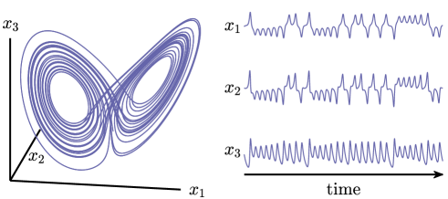
Figure 1: Chaotic Lorenz manifold. Lorenz attractor plotted in space (left) and time (right).

Next, we model the neural system as a recurrent neural network driven by our inputs

$$\frac{1}{\gamma}\dot{\bm{r}}=-\bm{r}+\bm{g}\left(A\bm{r}+B\bm{x}+\bm{d}\right),$$

where $\bm{r}$ is a real-valued vector of $N$ reservoir neuron states, $A$ is an $N\times N$ matrix of inter-neuron connections, $B$ is an $N\times 3$ matrix of connections from the inputs to the neurons, $\bm{d}$ is an $N\times 1$ bias vector, $\bm{g}$ is a scalar activation function applied entry-wise to its input arguments (hence mapping vectors to vectors), and $\gamma$ is a time constant.

Several prior studies use echo state Jaeger2010 and FORCE learning Sussillo2009 which allow reservoirs to predict a chaotic time series by modifying the inter-neuron connections. This modification can be accomplished by using the chaotic time series $\bm{x}(t)$ to drive the reservoir, thereby generating the reservoir time series $\bm{r}(t)$ (Fig. 2a,b). Here, $\bm{x}(t)$ and $\bm{r}(t)$ are $3\times T$ and $N\times T$ matrices, respectively, from numerically evolving the differential equations over $T$ time steps. By solving for a simple $3\times N$ readout matrix $W$ that uses linear combinations of reservoir states to approximate the input by minimizing the matrix 2-norm (see Supplement)

$$W=\operatorname*{argmin}_{W}\|W\bm{r}(t)-\bm{x}(t)\|_{2},$$

the output $\hat{\bm{x}}(t)=W\bm{r}(t)$ mimics the input $\bm{x}(t)$ (Fig. 2c). Finally, we close the feedback loop by substituting the output as the input to create the autonomous reservoir (Fig. 2d)

$$\frac{1}{\gamma}\dot{\bm{r}}^{\prime}=-\bm{r}^{\prime}+\bm{g}\left((A+BW)\bm{r}^{\prime}+\bm{d}\right),$$

whose evolution projects to a Lorenz-shaped attractor as $\bm{x}^{\prime}(t)=W\bm{r}^{\prime}(t)$ (Fig. 2e). Hence, reservoirs sustain representations of complex temporal information by learning to autonomously evolve along a chaotic attractor from example inputs.

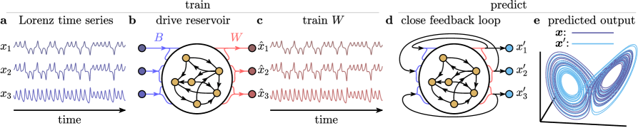
Figure 2: Representing chaotic attractors with reservoirs. (a) Time series of a chaotic Lorenz attractor that (b) drives the recurrent neural network reservoir. (c) Weighted sums of the reservoir states are trained to reproduce the original time series. (d) By using these weighted sums of reservoir states to drive the reservoir instead of the inputs, (e) the reservoir autonomously evolves along a trajectory that projects to a Lorenz-shaped chaotic manifold.

To study how reservoirs might perform computations by modifying the position or geometry of these representations in a desired way, we first adapt the framework to include a vector of control parameters $\bm{c}$ that map to the reservoir neurons through matrix $C$ to yield

$$\frac{1}{\gamma}\dot{\bm{r}}=-\bm{r}+\bm{g}\left(A\bm{r}+B\bm{x}+C\bm{c}+\bm{d}\right).$$

Such control parameters were also previously used to switch between multiple attractor outputs Sussillo2009 . The second adaptation is to approximate the reservoir dynamics using a Taylor series to quadratic order around equilibrium values $\bm{r}^{*},\bm{x}^{*}=\bm{0},\bm{c}^{*}=\bm{0}$, yielding

$$\frac{1}{\gamma}\delta\dot{\bm{r}}=-\delta\bm{r}+U(A\delta\bm{r}+B\bm{x}+C\bm{c})+V(A\delta\bm{r}+B\bm{x}+C\bm{c})^{2}.$$ (2)

Here, $\delta\bm{r}=\bm{r}-\bm{r}^{*}$, $U$, and $V$ are diagonal matrices whose $i$-th entries are the first and half of the second derivatives of $g_{i}$ evaluated at the fixed point, respectively, and $()^{2}$ is the entry-wise square of the vector (see Supplement for details). By studying quadratic reservoirs and how they learn to manipulate their representations of chaotic manifolds, we will gain an intuition due to their analytic tractability, and generalizability across many activation functions $\bm{g}$ when driven within a range over which the quadratic expansion is accurate.

III Learning a translation operation by example

Reservoirs learn complex information through simple imitation: approximating the driving inputs using the reservoir states is enough to autonomously represent and evolve about a chaotic manifold. Here we show that this simple scheme is also enough to learn to translate the representation. We begin with a Lorenz time series $\bm{x}_{0}(t)$, and create shifted copies

$$\bm{x}_{c}(t)=\bm{x}_{0}(t)+P\bm{c}.$$ (3)

For the purposes of demonstration, we consider a translation in the $x_{1}$ direction such that $P=[1;0;0]$ is a column vector, and $\bm{c}=0,1,2,3$ is a scalar. We use these four time series to drive our reservoir according to Eq. 2, thereby generating four reservoir time series $\bm{r}_{c}(t)$. Numerically, $\bm{x}_{c}(t)$ and $\bm{r}_{c}(t)$ are matrices of dimension $3\times T$ and $N\times T$ over $T$ time steps, which we concatenate along the time dimension into $\bm{x}(t)=[\bm{x}_{0}(t),\bm{x}_{1}(t),\bm{x}_{2}(t),\bm{x}_{3}(t)]$ and $\bm{r}(t)=[\bm{r}_{0}(t),\bm{r}_{1}(t),\bm{r}_{2}(t),\bm{r}_{3}(t)]$, respectively. Then, we compute output weights

$$W=\operatorname*{argmin}_{W}\|W\bm{r}(t)-\bm{x}(t)\|_{2},$$ (4)

such that our output $\hat{\bm{x}}=W\bm{r}(t)$ approximates our input $\bm{x}(t)$ (Fig. 3a–c). Finally, we substitute the output as the input to yield the feedback system (Fig. 3d)

$$\frac{1}{\gamma}\delta\dot{\bm{r}}^{\prime}=-\delta\bm{r}^{\prime}+U(R\delta\bm{r}^{\prime}+C\bm{c})+V(R\delta\bm{r}^{\prime}+C\bm{c})^{2},$$ (5)

where $R=A+BW$ (see Supplement for a discussion on $W\bm{r}_{c}(t)\approx W\delta\bm{r}_{c}(t)$).

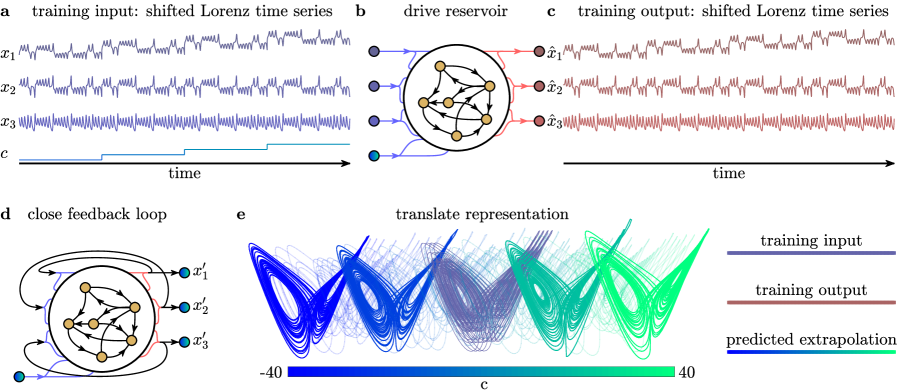
Figure 3: Learning and extrapolating a translation operation through examples. (a) Schematic of the time series of the Lorenz and control inputs, beginning with the original Lorenz time series $\bm{x}_{0}(t)$ at $\bm{c}=0$, followed by three equally spaced shifts in the $x_{1}$ direction and in the $\bm{c}$ parameter. (b) These inputs generate four reservoir time series $\bm{r}_{c}(t)$. (c) Next, weighted sums of the reservoir states are used to generate outputs $W\bm{r}_{c}(t)=\hat{\bm{x}}_{c}(t)\approx\bm{x}_{c}(t)$ that mimic the inputs. (d) The outputs $W\bm{r}(t)$ replace the inputs $\bm{x}(t)$ to create a reservoir with a closed feedback loop. (e) Over the course of a single simulation, the reservoir evolves autonomously about a Lorenz-shaped manifold, and translates this representation along $x_{1}$ by smoothly and continuously changing $\bm{c}$ as a real number over a range much larger than the training range.

As we evolve this autonomous reservoir while varying $\bm{c}$ to extreme values $-40\leq\bm{c}\leq 40$ both inside and outside of the training values, it has learned to evolve about a Lorenz-shaped manifold that is translated based on the value of $\bm{c}$ (see Supplement for translations in all spatial directions). Hence, by training the network on shifted copies of the input time series, the reservoir has learned a translation operation on the attractor.

IV Learning a linear transformation operation by example

In addition to learning a translation operation that does not change the geometry of the representation, here we demonstrate that reservoirs can learn linear transformation using the exact same framework. Similarly, we begin with a Lorenz time series $\bm{x}_{0}(t)$ generated from Eq. 1, and create linearly transformed copies of the time series such that

$$\bm{x}_{c}(t)=(I+cP)\bm{x}_{0}(t),$$ (6)

for $c=0,1,2,3$, where $P$ is a matrix encoding a transformation (Fig. 4a,c). Specifically, we perform a squeeze along $x_{1}$ by setting $[P]_{11}=-0.012$ and the remaining elements to 0.

Exactly as before, we drive the reservoir according to Eq. 2, concatenate our input and reservoir time series into $\bm{x}(t)$ and $\bm{r}(t)$ to train the output weights $W$ according to Eq. 4, and feed the outputs back as inputs to yield the feedback system Eq. 5. This reservoir autonomously evolves about a Lorenz-shaped manifold that stretches based on the parameter $-40\leq c\leq 40$ (Fig. 4b,d) far outside of the parameters used in the training regime $c=0,1,2,3$ (see Supplement for more examples). Hence, using the same framework, the reservoir has learned the linear transformation operation on the attractor manifold.

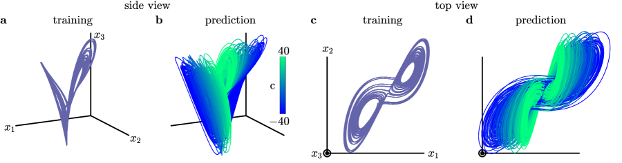
Figure 4: Extrapolating a transformation operation through examples. (a) 3-dimensional plot of the training data of the Lorenz time series that has been stretched along the $x_{1}$ direction at $c=0,1,2,3$. (b) 3-dimensional plot of the feedback reservoir output that autonomously evolves about a Lorenz-shaped manifold that stretches dramatically based on varying $c$ from $-40$ to $40$. We also provide a top view of the (c) training data and (d) predicted output data.

V Learning to infer a bifurcation by example

For both translations and transformations, the reservoir learned a smooth change in its representation of the chaotic manifold. Here we demonstrate that a reservoir can infer, without actually ever having experienced, a much more dramatic change: a bifurcation. In the Lorenz attractor (Eq. 1 for $\rho>1,\sigma=10,\beta=8/3$), there are two fixed points: one at the center of each wing, which undergo a subcritical Hopf bifurcation when $\rho=\rho^{*}\approx 24.7$ Strogatz1994 . When $\rho<\rho^{*}$, these two fixed points are stable. When $\rho>\rho^{*}$, the fixed points become unstable, yielding the characteristic wing-shaped flow. Here we demonstrate that a reservoir trained only on stable examples ($\rho<\rho^{*}$) can accurately predict the unstable flow ($\rho>\rho^{*}$).

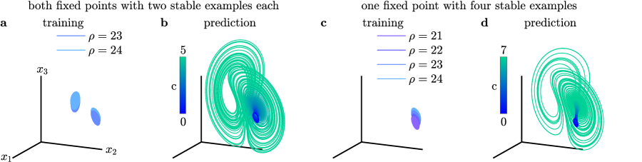
Figure 5: Extrapolating the bifurcation of the Lorenz. (a) Two training trajectories for each of the stable Lorenz fixed points at the wings, for $\rho=23$ with $c=0$ (blue) and for $\rho=24$ with $c=1$ (light blue). (b) The predicted trajectory of the feedback reservoir moves towards a stable fixed point for $c=0$, and bifurcates into a Lorenz-shaped manifold as $c$ is increased. (c) Four training examples for one of the stable Lorenz fixed points for $\rho=21,22,23,24$ with $c=0,1,2,3$. (d) The predicted trajectory moves towards a stable fixed point for $c=0$, and then bifurcates into a Lorenz-shaped manifold as $c$ is increased.

For the two fixed points $\bm{a}$ and $\bm{b}$, we begin with four training trajectories: $\bm{x}^{a}_{23}(t)$ and $\bm{x}^{b}_{23}(t)$ that evolve stably towards the fixed points for $\rho=23$, and $\bm{x}^{a}_{24}(t)$ and $\bm{x}^{b}_{24}(t)$ that evolve stably towards the fixed points for $\rho=24$ (Fig. 5a). We then drive the reservoir with $\bm{x}^{a}_{23}(t)$ and $\bm{x}^{b}_{23}(t)$ while setting $c=0$, and with $\bm{x}^{a}_{24}(t)$ and $\bm{x}^{b}_{24}(t)$ while setting $c=1$, and train the output weights. Finally, we evolve the feedback reservoir while changing $c$ from $0$ to $5$, and note that the trajectory bifurcates into a Lorenz-shaped manifold (Fig. 5b).

As a second demonstration, we begin with another set of four training trajectories: $\bm{x}^{a}_{21}(t),\dotsm,\bm{x}^{a}_{24}(t)$ that evolve stably towards only one fixed point for $\rho=21,\dotsm,24$ (Fig. 5c). We then drive the reservoir with $\bm{x}^{a}_{21}(t),\dotsm,\bm{x}^{a}_{24}(t)$ while setting $c=0,\dotsm,3$, and train the output weights. Finally, we evolve the feedback reservoir while changing $c$ from $0$ to $7$, and note that the trajectory again bifurcates into a Lorenz-shaped manifold (Fig. 5d). Hence, after only observing a few stable trajectories before the bifurcation ($\rho<\rho^{*}$), the reservoir accurately extrapolates the geometry of the Lorenz trajectory after the bifurcation ($\rho>\rho^{*}$).

VI Mechanism of how operations are learned

Now that we have taught reservoirs to manipulate chaotic manifolds, we seek to understand the mechanism. We begin with some intuition by expanding the feedback dynamics

$$\frac{1}{\gamma}\delta\dot{\bm{r}}^{\prime}=([U+\underbrace{2V~{}\mathrm{diag}(C\bm{c})}_{\mathrm{stretch}}]R-I)\delta\bm{r}^{\prime}+\underbrace{UC\bm{c}}_{\mathrm{shift}}+V(R\delta\bm{r}^{\prime})^{2}+\underbrace{V(C\bm{c})^{2}}_{\mathrm{small}},$$

and notice that the control parameter can scale the shape of the reservoir’s internal dynamics (stretch), and add a constant driving input (shift). For small changes in $\bm{c}$, the quadratic term $C\bm{c}$ is negligible. To formalize this intuition, we consider the time series $\bm{r}^{\prime}(t)=\bm{r}^{\prime}_{c=0}(t)$ generated by evolving the autonomous reservoir according to Eq. 5 at $\bm{c}=\bm{0}$. Next, we take the total differential of Eq. 5 evaluated at $\bm{r}^{\prime}(t)$ and $\bm{c}=\bm{0}$ to yield

$$(I-KA)d\bm{r}^{\prime}+\frac{1}{\gamma}d\dot{\bm{r}}^{\prime}=K(BWd\bm{r}^{\prime}+Cd\bm{c}),$$ (7)

where $K=U+2V~{}\mathrm{diag}(R\delta\bm{r}^{\prime}(t))$. Our goal is to write the change in the reservoir state $d\bm{r}^{\prime}(t)$ that is induced by changing the control parameter by an infinitesimal amount $d\bm{c}$.

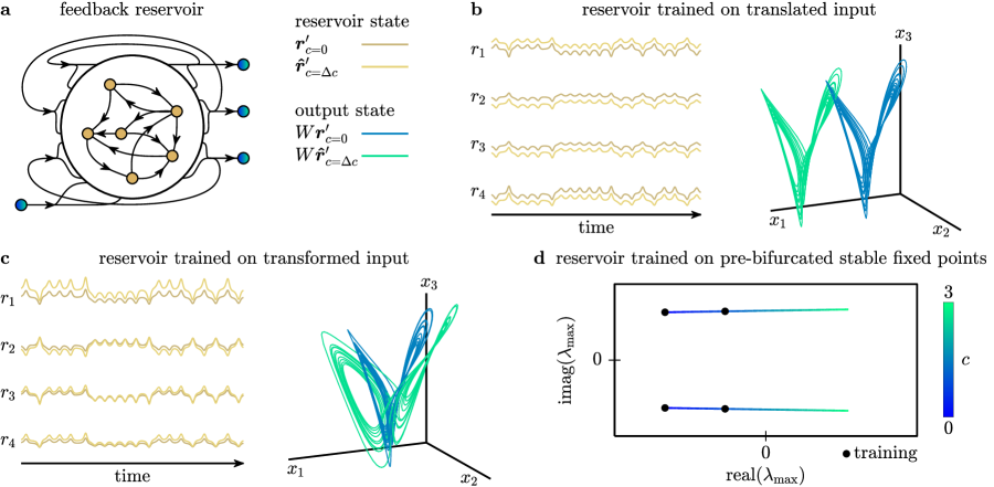
Figure 6: Changing the control parameter changes the reservoir dynamics to manipulate representations. (a) Schematic of a reservoir with feedback connections after the output weights $W$ have been trained. (b) Reservoir time series generated by evolving the autonomous reservoir with the original Lorenz input with $\bm{c}=0$ (dark gold). We also show the predicted time series from solving Eq. 8 after training on translated examples and setting $d\bm{c}=\Delta\bm{c}=20$ (light gold). The output projections of the two time series are shown in blue and green, respectively. (c) The original and predicted reservoir states and their output projections for $\Delta c=-40$ after training on transformed Lorenz inputs by solving Eq. 9. (d) Plot of the real and imaginary components of the two most unstable eigenvalues of the autonomous reservoir trained on two stable Lorenz trajectories (Fig. 5a,b). The reservoir is linearized about its fixed point according to Eq. 10 as $c$ is slowly changed.

When learning translations, the output weights are trained such that $W\bm{r}_{c}(t)\approx\bm{x}_{c}(t)=\bm{x}(t)+P\bm{c}$. For sufficiently nearby training examples (small $P,\bm{c}$), we also implicitly approximate the differential relation $Wd\bm{r}(t)\approx Pd\bm{c}$. Additionally, if the feedback reservoir stabilizes these examples, then $Wd\bm{r}^{\prime}(t)\approx Pd\bm{c}$. Substituting this relation into Eq. 7 yields

$$(I-KA)d\bm{r}^{\prime}+\frac{1}{\gamma}d\dot{\bm{r}}^{\prime}\approx K(BP+C)d\bm{c}.$$

If we fix $d\bm{c}$, we have $2N$ variables, $d\bm{r}^{\prime}$ and $d\dot{\bm{r}}^{\prime}$, but only $N$ equations. By taking the time derivative of the differential relation, we generate another $N$ variables and $N$ equations. Continuing to take time derivatives yields the following system of equations

$$\begin{bmatrix}H_{0}&H_{-1}&0&\dotsm\\ H_{1}&H_{0}&H_{-1}&\dotsm\\ H_{2}&2H_{1}&H_{0}&\dotsm\\ \vdots&\vdots&\vdots&\ddots\end{bmatrix}\begin{bmatrix}d\bm{r}^{\prime}\\ d\dot{\bm{r}}^{\prime}\\ d\ddot{\bm{r}}^{\prime}\\ \vdots\end{bmatrix}\approx\begin{bmatrix}K\\ \dot{K}\\ \ddot{K}\\ \vdots\end{bmatrix}(BP+C)d\bm{c},$$

where $H_{-1}=\frac{1}{\gamma}I$, $H_{0}=I-KA$, and $H_{i}=-K^{(i)}A$ is the $i$-th time-derivative of $KA$. This matrix is a block-Hessenberg matrix, with an analytic solution Sowik2018 for the first term $d\bm{r}^{\prime}$. We truncate this solution (see Supplement) to explicitly relate $d\bm{c}$ to $d\bm{r}^{\prime}$ as follows:

$$d\bm{r}^{\prime}\approx-\begin{bmatrix}\gamma H_{0}^{2}-H_{1}\end{bmatrix}^{-1}\begin{bmatrix}-\gamma H_{0}&~{}I\end{bmatrix}\begin{bmatrix}K\\ \dot{K}\end{bmatrix}(BP+C)d\bm{c}.$$ (8)

As a demonstration, we pick a finite $\Delta\bm{c}=20$, and plot the original and predicted change in the reservoir states, and their outputs in spatial coordinates (Fig. 6b). Hence, using only the feedback dynamics Eq. 5 and sufficiently nearby training examples, changing $\bm{c}$ causes changes in the reservoir states from Eq. 8 that map to a translation.

The same approach can be used for linear transformations, where the output weights are trained such that $W\bm{r}_{c}(t)\approx\bm{x}_{c}(t)=(I+cP)\bm{x}(t)$. For sufficiently nearby training examples, we implicitly approximate the differential relation $Wd\bm{r}(t)\approx P\bm{x}(t)dc\approx PW\bm{r}(t)dc$, which if properly stabilized, yields $Wd\bm{r}^{\prime}(t)\approx PW\bm{r}^{\prime}(t)$. Performing the same time derivatives and solution truncation as in the translation, we get the following relation between $dc$ and $d\bm{r}^{\prime}$:

$$d\bm{r}^{\prime}\approx-\begin{bmatrix}\gamma H_{0}^{2}-H_{1}\end{bmatrix}^{-1}\begin{bmatrix}-\gamma H_{0}&~{}I\end{bmatrix}\begin{bmatrix}K(BPW\bm{r}^{\prime}+C)\\ \dot{K}(BPW\bm{r}^{\prime}+C)+KBPW\dot{\bm{r}}^{\prime}\end{bmatrix}dc.$$ (9)

As another demonstration, we set $\Delta c=-40$, and plot the original and predicted change in the reservoir states, and their outputs (Fig. 6c).

Finally, to understand how the reservoir is able to infer a bifurcation, we demonstrate that it learns a smooth translation of eigenvalues. Specifically, at $\rho^{*}$, the fixed points at the wings of the Lorenz system undergo a Hopf bifurcation, whereby the real component of complex conjugate eigenvalues goes from negative to positive. To track the eigenvalues of the autonomous reservoir, we linearize Eq. 5 about a fixed point $\delta\bm{r}^{*}$ such that

$$\frac{1}{\gamma}\delta\dot{\bm{r}}^{\prime}\approx[-I+UR+2V\mathrm{diag}(R\delta\bm{r}^{*}+C\bm{c})R](\delta\bm{r}^{\prime}-\delta\bm{r}^{*}).$$ (10)

Then, using the output weights trained only on stable Lorenz trajectories (at $c=0,\rho=23$ and $c=1,\rho=24$; Fig. 5a,b), we track the autonomous reservoir’s two most unstable eigenvalues (largest real component) at the fixed point as we vary the control parameter from $c=0$ to $c=3$. We find that these eigenvalues are complex conjugates whose real components go from negative to positive (Fig. 6d). Hence, we demonstrate that not only can reservoirs learn smooth translations and transformations by mapping $d\bm{c}$ to $d\bm{r}^{\prime}$, but they can also perform bifurcations by learning smooth changes in their eigenvalues.

VII Simultaneous learning of multiple operations

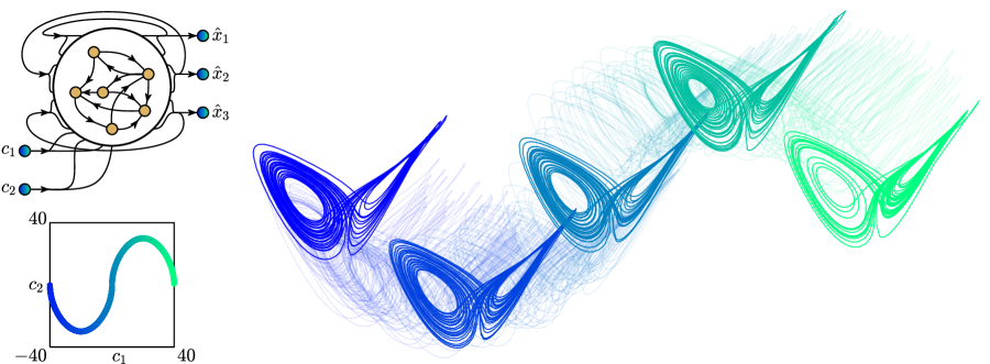
Figure 7: Flight of the Lorenz. A reservoir trained on translated inputs along the $x_{1}$ and $x_{3}$ directions evolves autonomously along a Lorenz-shaped chaotic manifold. We can change the $x_{1}$ and $x_{3}$ position of its representation by changing control parameters $c_{1}$ and $c_{2}$, respectively.

To close, here we demonstrate that reservoirs can easily learn multiple computations by changing multiple control inputs. We train a translation in the $x_{1}$ direction with control parameter $c_{1}$, and a translation in the $x_{3}$ direction with control parameter $c_{2}$. As before, we begin with a Lorenz time series $\bm{x}_{0,0}(t)$ generated from Eq. 1, and created shifted copies

$$\bm{x}_{c_{1},c_{2}}(t)=\bm{x}_{0,0}(t)+c_{1}\bm{a}_{1}+c_{2}\bm{a}_{2},$$

where $\bm{a}_{1}=[1;0;0]$ corresponds to an $x_{1}$ shift, and $\bm{a}_{2}=[0;0;1]$ corresponds to an $x_{3}$ shift. We generate 10 shifted inputs, with one unshifted attractor ($c_{1}=0,c_{2}=0$), three shifts in the $x_{1}$ direction ($c_{1}=1,2,3,c_{2}=0$), three shifts in the $x_{3}$ direction ($c_{1}=0,c_{2}=1,2,3$), and three shifts in both directions ($c_{1}=1,2,3,c_{2}=1,2,3$). We use these shifted copies along with their corresponding control inputs to drive our reservoir and produce 10 reservoir time series $\bm{r}_{c_{1},c_{2}}(t)$. Then, we concatenate these 10 time series into $\bm{x}(t)$ and $\bm{r}(t)$ to train output weights $W$ according to Eq. 4, and perform the feedback according to Eq. 5 where $\bm{c}=[c_{1};~{}c_{2}]$ is a vector. By changing parameters $c_{1}$ and $c_{2}$, the reservoir evolves about a Lorenz-shaped manifold that is shifted in the $x_{1}$ and $x_{3}$ directions (Fig. 7).

VIII Discussion

In this paper, we teach an RNN to evolve about a Lorenz-shaped manifold, and to control its evolution about a translated, transformed, and bifurcated continua of such manifolds. Our approach contributes to prior work on artificial neural networks in three significant ways Seung1998learning ; Wu2016 ; Jaeger2010 ; Sussillo2009 . First, we provide a means by which a neural system can learn continuous interpolated and extrapolated modifications, along with discontinuous bifurcations, of its own representation solely through examples. Second, the learned manifolds are spatially and temporally complex, allowing for potential extensions to learning modifications of time series data such as speech or music with a structured yet unpredictable evolution. Third, we use a randomly generated and arbitrarily connected network that does not need to be artificially engineered to preserve invariance or manipulate information Wu2016 .

One of the main limitations of this work is the lack of a clear mechanism of how the network connectivity ultimately stabilizes the chaotic manifold. Much progress has been made in tackling this limitation, both by exercising theoretical concepts of generalized synchronization Rulkov1995 , and by developing tools for controlling chaos Ott1990 . However, there is insufficient knowledge to guarantee that a set of training and reservoir parameters will always successfully teach the desired computation. Similarly, we are unable to specify exactly how far to space the training examples for the feedback reservoir to successfully learn the linear relationships between the differential of the reservoir states and the control parameter.

A particularly promising area for future work is related to the simple quadratic form of the reservoir. Because all of these results are obtained by driving our reservoir in the quadratic regime, the same results should hold for common neural mass models, such as the Wilson-Cowan model Wilson1972 . Hence, these results may provide a unifying framework for learning and computing in dynamical neural models. Additionally, these results provide a basis for exploring more complex computations, such as inferring bifurcations in experimental data, and testing the reservoir’s “imagination” in reconstructing more complex chaotic manifolds using incomplete data. Finally, and perhaps most astonishingly, the reservoir’s ability to accurately reconstruct the full nonlinear geometry of the bifurcated Lorenz manifold after only observing pre-bifurcation data implies that it is not only imitating examples, but actually inferring higher-order nonlinear structure. This work therefore provides a starting point for exploring exactly how higher-order structure is learned by neural systems.

IX Acknowledgments

We are thankful for the insightful feedback and comments from Harang Ju and Keith Wiley. We gratefully acknowledge support from the John D. and Catherine T. MacArthur Foundation, the Alfred P. Sloan Foundation, the ISI Foundation, the Paul Allen Foundation, the Army Research Laboratory (No. W911NF-10-2-0022), the Army Research Office (Nos. Bassett-W911NF-14-1-0679, Grafton-W911NF-16-1-0474, and DCIST-W911NF-17-2-0181), the Office of Naval Research (ONR), the National Institute of Mental Health (Nos. 2-R01-DC-009209-11, R01-MH112847, R01-MH107235, and R21-M MH-106799), the National Institute of Child Health and Human Development (No. 1R01HD086888-01), National Institute of Neurological Disorders and Stroke (No. R01 NS099348), and the National Science Foundation (NSF) (Nos. DGE-1321851, BCS-1441502, BCS-1430087, NSF PHY-1554488, and BCS-1631550). The content is solely the responsibility of the authors and does not necessarily represent the official views of any of the funding agencies.

X Citation Diversity Statement

Recent work in several fields of science has identified a bias in citation practices such that papers from women and other minorities are under-cited relative to other papers in the field Dworkin2020 . Here we sought to proactively consider choosing references that reflect the diversity of our field in thought, form of contribution, gender, and other factors. We classified gender based on the first names of the first and last authors, with possible combinations including male/male, male/female, female/male, and female/female. We regret that our current methodology is limited to consideration of gender as a binary variable. Excluding self-citations to the first and senior authors of our present paper, the references contain 50% male/male, 23.5% male/female, 11.8% female/male, and 14.7% female/female categorizations. We look forward to future work that will help us to better understand how to support equitable practices in science.

XI References

References

- (1) Nvidia. Nvidia V100 Tensor Core GPU (2020). URL https://images.nvidia.com/content/technologies/volta/pdf/volta-v100-datasheet-update-us-1165301-r5.pdf.
- (2) Intel Corporation. and Generation Intel Core Processor Families, Volume 1 of 2 (2019). URL https://www.intel.com/content/www/us/en/products/docs/processors/core/8th-gen-core-family-datasheet-vol-1.html. Rev. 003.
- (3) von Neumann, J. First draft of a report on the EDVAC. IEEE Annals of the History of Computing 15, 27–75 (1993).
- (4) Alglave, J. et al. The semantics of power and ARM multiprocessor machine code. In Proceedings of the 4th workshop on Declarative aspects of multicore programming - DAMP ’09, 13 (ACM Press, New York, New York, USA, 2008).
- (5) Zhang, Z., Jiao, Y.-Y. & Sun, Q.-Q. Developmental maturation of excitation and inhibition balance in principal neurons across four layers of somatosensory cortex. Neuroscience 174, 10–25 (2011).
- (6) Faulkner, R. L. et al. Development of hippocampal mossy fiber synaptic outputs by new neurons in the adult brain. Proceedings of the National Academy of Sciences 105, 14157–14162 (2008).
- (7) Dunn, F. A. & Wong, R. O. L. Diverse Strategies Engaged in Establishing Stereotypic Wiring Patterns among Neurons Sharing a Common Input at the Visual System’s First Synapse. Journal of Neuroscience 32, 10306–10317 (2012).
- (8) Craik, F. I. & Bialystok, E. Cognition through the lifespan: mechanisms of change. Trends in Cognitive Sciences 10, 131–138 (2006).
- (9) Tacchetti, A., Isik, L. & Poggio, T. A. Invariant Recognition Shapes Neural Representations of Visual Input. Annual Review of Vision Science 4, 403–422 (2018).
- (10) Moser, E. I., Kropff, E. & Moser, M.-B. Place Cells, Grid Cells, and the Brain’s Spatial Representation System. Annual Review of Neuroscience 31, 69–89 (2008).
- (11) Ifft, P. J., Shokur, S., Li, Z., Lebedev, M. A. & Nicolelis, M. A. L. A Brain-Machine Interface Enables Bimanual Arm Movements in Monkeys. Science Translational Medicine 5, 210ra154–210ra154 (2013).
- (12) Sainath, T. N. et al. Deep Convolutional Neural Networks for Large-scale Speech Tasks. Neural Networks 64, 39–48 (2015).
- (13) Jarrell, T. A. et al. The Connectome of a Decision-Making Neural Network. Science 337, 437–444 (2012).
- (14) Lee, J. & Tashev, I. High-level feature representation using recurrent neural network for speech emotion recognition. In Proceedings of the Annual Conference of the International Speech Communication Association, INTERSPEECH, vol. 2015-Janua, 1537–1540 (2015).
- (15) Wang, J., Narain, D., Hosseini, E. A. & Jazayeri, M. Flexible timing by temporal scaling of cortical responses. Nature Neuroscience 21, 102–110 (2018).
- (16) Weber, M., Maia, P. D. & Kutz, J. N. Estimating Memory Deterioration Rates Following Neurodegeneration and Traumatic Brain Injuries in a Hopfield Network Model. Frontiers in Neuroscience 11 (2017).
- (17) Burak, Y. & Fiete, I. R. Accurate Path Integration in Continuous Attractor Network Models of Grid Cells. PLoS Computational Biology 5, e1000291 (2009).
- (18) Yoon, K. et al. Specific evidence of low-dimensional continuous attractor dynamics in grid cells. Nature Neuroscience 16, 1077–1084 (2013).
- (19) Hegarty, M. Mechanical reasoning by mental simulation. Trends in Cognitive Sciences 8, 280–285 (2004).
- (20) Kubricht, J. R., Holyoak, K. J. & Lu, H. Intuitive Physics: Current Research and Controversies. Trends in Cognitive Sciences 21, 749–759 (2017).
- (21) Pfeiffer, B. E. & Foster, D. J. Hippocampal place-cell sequences depict future paths to remembered goals. Nature 497, 74–79 (2013).
- (22) Gold, J. I. & Shadlen, M. N. The Neural Basis of Decision Making. Annual Review of Neuroscience 30, 535–574 (2007).
- (23) Strogatz, S. H. Nonlinear Dynamics and Chaos (Perseus Books, 1994), 1 edn.
- (24) Yang, J., Wang, L., Wang, Y. & Guo, T. A novel memristive Hopfield neural network with application in associative memory. Neurocomputing 227, 142–148 (2017).
- (25) Wu, S., Wong, K. Y. M., Fung, C. C. A., Mi, Y. & Zhang, W. Continuous Attractor Neural Networks: Candidate of a Canonical Model for Neural Information Representation. F1000Research 5, 156 (2016).
- (26) Graves, A. et al. Hybrid computing using a neural network with dynamic external memory. Nature 538, 471–476 (2016).
- (27) Carroll, J. M. Letter knowledge precipitates phoneme segmentation, but not phoneme invariance. Journal of Research in Reading 27, 212–225 (2004).
- (28) Fee, M. S. & Scharff, C. The Songbird as a Model for the Generation and Learning of Complex Sequential Behaviors. ILAR Journal 51, 362–377 (2010).
- (29) Donnay, G. F., Rankin, S. K., Lopez-Gonzalez, M., Jiradejvong, P. & Limb, C. J. Neural Substrates of Interactive Musical Improvisation: An fMRI Study of ‘Trading Fours’ in Jazz. PLoS ONE 9, e88665 (2014).
- (30) Qiao, J., Li, F., Han, H. & Li, W. Growing Echo-State Network With Multiple Subreservoirs. IEEE Transactions on Neural Networks and Learning Systems 28, 391–404 (2017).
- (31) Lorenz, E. N. Deterministic Nonperiodic Flow. Journal of the Atmospheric Sciences 20, 130–141 (1963).
- (32) Jaeger, H. The “ echo state ” approach to analysing and training recurrent neural networks – with an Erratum note. GMD Report 1, 1–47 (2010).
- (33) Sussillo, D. & Abbott, L. Generating Coherent Patterns of Activity from Chaotic Neural Networks. Neuron 63, 544–557 (2009).
- (34) Słowik, R. Inverses and Determinants of Toeplitz-Hessenberg Matrices. Taiwanese Journal of Mathematics 22, 901–908 (2018).
- (35) Seung, H. S. Learning continuous attractors in recurrent networks. In Advances in Neural Information Processing Systems, 654–660 (MIT Press, 1998).
- (36) Rulkov, N. F., Sushchik, M. M., Tsimring, L. S. & Abarbanel, H. D. I. Generalized synchronization of chaos in directionally coupled chaotic systems. Physical Review E 51, 980–994 (1995).
- (37) Ott, E., Grebogi, C. & Yorke, J. A. Controlling chaos. Physical Review Letters 64, 1196–1199 (1990).
- (38) Wilson, H. R. & Cowan, J. D. Excitatory and Inhibitory Interactions in Localized Populations of Model Neurons. Biophysical Journal 12, 1–24 (1972).
- (39) Dworkin, J. D. et al. The extent and drivers of gender imbalance in neuroscience reference lists. bioRxiv (2020).