Tsinghua Science and Technology, xxxxx 20xx, 2x(x): xxx–xxx\headoddnameZiheng Duan et al.: Multivariate Time Series Forecasting with Transfer Entropy Graph
TSINGHUA SCIENCE AND TECHNOLOGY
I S S N l l 1 0 0 7 - 0 2 1 4 0 ? / ? ? p p ? ? ? – ? ? ?
DOI: 1 0 . 2 6 5 9 9 / T S T . 2 0 2 1 . 9 0 1 0 0 8 1
V o l u m e xx, N u m b e r x, x x x x x x x 2 0 x x
Multivariate Time Series Forecasting with Transfer Entropy Graph
Ziheng Duan, Haoyan Xu, Yida Huang, Jie Feng, Yueyang Wang∗
|
Abstract: Multivariate time series (MTS) forecasting is an essential problem in many fields. Accurate forecasting results can effectively help decision-making. To date, many MTS forecasting methods have been proposed and widely applied. However, these methods assume that the predicted value of a single variable is affected by all other variables, which ignores the causal relationship among variables. To address the above issue, we propose a novel end-to-end deep learning model, termed graph neural network with Neural Granger Causality (CauGNN) in this paper. To characterize the causal information among variables, we introduce the Neural Granger Causality graph in our model. Each variable is regarded as a graph node, and each edge represents the casual relationship between variables. In addition, convolutional neural network (CNN) filters with different perception scales are used for time series feature extraction, which is used to generate the feature of each node. Finally, Graph Neural Network (GNN) is adopted to tackle the forecasting problem of graph structure generated by MTS. Three benchmark datasets from the real world are used to evaluate the proposed CauGNN. The comprehensive experiments show that the proposed method achieves state-of-the-art results in the MTS forecasting task.
Key words: Multivariate Time Series Forecasting; Neural Granger Causality Graph; Transfer Entropy |
| Ziheng Duan and Yueyang Wang are with the School of Big Data and Software Engineering, Chongqing University, Chongqing 401331, China. E-mail: duanziheng@zju.edu.cn, yueyangw@cqu.edu.cn | |
| Haoyan Xu, Yida Huang and Jie Feng are with the Department of Control Science and Engineering, Zhejiang University, Hangzhou 310027, China. E-mail: {haoyanxu, stevenhuang, zjucse_fj}@zju.edu.cn | |
| Corresponding author. | |
| Manuscript received: 23-Sep-2021; accepted: 22-Oct-2021 |
1 Introduction
In the real world, multivariate time series (MTS) data are common in various fields [1], such as the sensor data in the Internet of things, the traffic flows on highways, and the prices collected from stock markets (e.g., metals price) [2]. In recent years, many time series forecasting methods have been widely studied and applied [3]. For univariate situations, autoregressive integrated moving average model (ARIMA) [4] is one of the most classic forecasting methods. However, due to the high computational complexity, ARIMA is not suitable for multivariate situations. VAR [5, 6, 4] method is an extended multivariate version of the AR model, which is widely used in MTS forecasting tasks due to its simplicity. But it cannot handle the nonlinear relationships among variables, which reduces its forecasting accuracy.
In addition to traditional statistical methods, deep learning methods are also applied for the MTS forecasting problem [7]. The recurrent neural network (RNN) [8] and its two improved versions, namely the long short term memory (LSTM) [9] and the gated recurrent unit (GRU) [10], realize the extraction of time series dynamic information through the memory mechanism. LSTNet [11] encodes short-term local information into low dimensional vectors using 1D convolutional neural networks and decodes the vectors through a recurrent neural network. However, the existing deep learning methods cannot model the pairwise causal dependencies among MTS variables explicitly. For example, the future traffic flow of a specific street is easier to be influenced and predicted by the traffic information of the neighboring area. In contrast, the knowledge of the area farther away is relatively useless [12]. If such prior causal information can be considered, it is more conducive to the interaction among variables with causality.
Granger causality analysis (G-causality) [13, 14] is one of the most famous studies on the quantitative characterization of time series causality. However, as a linear model, G-causality cannot well handle nonlinear relationships. Then transfer entropy (TE) [15] is proposed for causal analysis, which can deal with the nonlinear cases. TE has been widely used in the economic [16], biological [17] and industrial [18] fields.
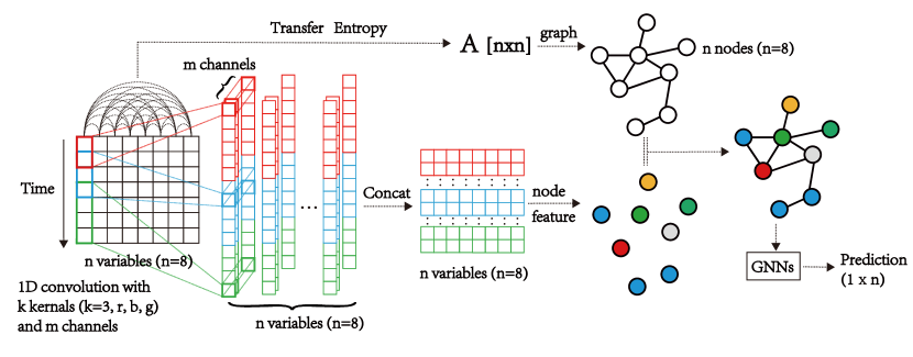
We propose a novel framework called Graph Neural Network with Causality (CauGNN) to further address the above limitation for MTS forecasting tasks. After the pairwise TE among variables is calculated, the TE matrix can be obtained, regarded as the adjacency matrix of the graph structure. Each variable is one node of this graph. In addition, CNN filters with different perception scales are used for time series feature extraction, which is used to generate the feature of each node. Finally, Graph Neural Network (GNN) is adopted to tackle the embedding and forecasting problem of the graph generated by MTS. Our major contributions are:
-
•
To the best of our knowledge, we first propose an end-to-end deep learning framework that considers multivariate time series as a graph structure with causality.
-
•
We use transfer entropy to extract the causality among time series and construct the TE graph as a priori information to guide the forecasting task.
-
•
We conduct extensive experiments on MTS benchmark datasets, and the results have proved that CauGNN outperforms the state-of-the-art models.
2 PRELIMINARIES
2.1 Neural Granger Causality
Neural Granger is an improved Granger causality inference method. It inherits the core idea of Granger causality, that is, if the addition of historical information of variable significantly improves the prediction accuracy of another variable , then variable is the cause of variable , and vice versa. The difference is that the traditional linear Granger method uses the AR model for prediction. In contrast, the neural Granger uses deep learning and regularization to take the nonlinearity into account and avoids the computational complexity caused by pairwise calculation.
The Neural Granger network structure consists of two parts, including the variable selection module and prediction module. The variable selection module is a fully connected layer that directly accepts historical time series as input. The neural Granger method selects key variables by adding group Lasso regularization constraints to the weight parameters of this layer. Group Lasso is an evolved version of Lasso regularization, which can divide constrained parameters into multiple subgroups. If a specific group is not significant for prediction, the entire group of parameters will be assigned a zero value. The variable selection module sets the weights connected to an input variable at different time points as a group. If the weights of the subgroup are not zero under the regularization constraint, it means that the variable has a significant effect on prediction. It is thus determined as the cause of the variable to be predicted. The second part of the Neural Granger is the prediction layer. This part is not significantly different from the general prediction method. Networks such as multilayer perceptron or LSTM can be used. For each variable , a neural Granger network is established to find its cause variables. The objective function of the network is as follows.
| (1) |
where is the true value of the variable at time , is the value of all variables in lags, is the function that specifies how lags from 1 to affect the future evolution of the series, is the observed time points, is the number of variables, is the regularization coefficient, represents all the weight parameter connected with the -th variable in the variable selection module and is the F-norm.
2.2 Graph Neural Network
The concept of graph neural network (GNN) was first proposed in [19], which extended existing neural networks for processing the data represented in graph domains. A wide variety of graph neural network (GNN) models have been proposed in recent years [20, 21]. Most of these approaches fit within the framework of “neural message passing” proposed by Gilmeret et al.[22]. In the message passing framework, a GNN is viewed as a message passing algorithm where node representations are iteratively computed from the features of their neighbor nodes using a differentiable aggregation function [23, 24, 25].
A separate line of work focuses on generalizing convolutions to graphs. The Graph Convolutional Networks (GCN) [26] could be regarded as an approximation of spectral-domain convolution of the graph signals. GCN convolutional operation could also be viewed as sampling and aggregating of the neighborhood information, such as GraphSAGE [27] and FastGCN [28], enabling training in batches while sacrificing some time-efficiency. Coming right after GCN, Graph Isomorphism Network (GIN) [29] and k-GNNs [30] is developed, enabling more complex forms of aggregation. Graph Attention Networks (GAT) [31] is another nontrivial direction to go under the topic of graph neural networks. It incorporates attention into propagation, attending over the neighbors via self-attention. Recently, researchers have also applied GNN to time series forecasting problem. For example, a correlational graph attention-based Long Short-Term Memory network (CGA-LSTM) was proposed in [32] and shows comparable performance. This further reminds us of the superiority of the graph method in the task of MTS forecasting.
3 Methodology
3.1 Problem Formulation
Given a matrix consisting of multiple observed time series , where and is the number of variables, the goal of MTS forecasting is to predict , where is the horizon ahead of the current time stamp.
3.2 Causality Graph Structure with Transfer Entropy
Transfer entropy (TE) is a measure of causality based on information theory, which was proposed by Schreiber in 2000 [33]. Given a variable , its information entropy is defined as:
| (2) |
where denotes all possible values of variable . Information entropy is used to measure the amount of information. A larger indicates that the variable contains more information. Conditional entropy is another information theory concept. Given two variables and , it is defined as:
| (3) |
where conditional entropy represents the information amount of under the condition that the variable is known. The TE of variables to is defined as:
| (4) |
where and represent their values at time . and . It can be found that TE is actually an increase in the information amount of the variable when changes from unknown to known. TE indicates the direction of information flow, thus characterizing causality. It is worth noting that TE is asymmetric, so the causal relationship between and is usually further indicated in the following way:
| (5) |
When is greater than , it means that is the cause of , otherwise is the consequence of . In this paper, we use neural granger to characterize the causal relationship among variables. The causality matrix of the multivariate time series can be formulated with the element corresponding to the -th row and -th column as:
| (6) |
where is the -th variable of , is the threshold to determine whether the causality is significant. can be regarded as the adjacency matrix of the MTS graph structure.
3.3 Feature Extraction of Multiple Receptive Fields
Time series is a special kind of data. When analyzing time series, it is necessary to consider not only its numerical value but also its trend over time. In addition, time series from the real world often have multiple meaningful periods. For example, the traffic flow of a certain street not only shows a similar trend every day, but meaningful rules can also be observed in the unit of a week. Therefore, it is reasonable to extract the features of time series in units of multiple certain periods. In this paper, we use multiple CNN filters with different receptive fields, namely kernel sizes, to extract features at multiple time scales. Given an input time series and CNN filters, denoted as , with different convolution kernel sizes are separately generated and the features are extracted as follows: , . denotes the convolution operation, represents the concatenate operation, and is a nonlinear activation function .
3.4 Node Embedding Based on Causality Matrix
After feature extraction, the input MTS is converted into a feature matrix , where is the number of features after the calculation introduced in Section 3.3. can be regarded as a feature matrix of a graph with nodes. The adjacency of nodes in the graph structure is determined by the causality matrix . For such graph structure, graph neural networks can be directly applied for the embedding of nodes. Inspired by k-GNNs [30] model, we propose CauGNN model and use the following propagation mechanism for calculating the forward-pass update of a node denoted by :
| (7) |
where and are parameter matrices, is the hidden state of node in the layer and denotes the neighbors of node . k-GNNs only perform information fusion between a certain node and its neighbors, ignoring the information of other non-neighbor nodes. This design highlights the relationship among variables, which can effectively avoid the information redundancy brought by high dimensions. By adding the priori causal information obtained by TE, the model does not need to find out the key variables for forecasting by itself. In this paper, the output dimension of the last graph neural network layer is 1, which is used as the prediction result.
Overall, we use -norm loss to measure the prediction of and optimize the model via Adam algorithm [34].
4 Experiments
In this section, we conduct extensive experiments on three benchmark datasets for multivariate time series forecasting tasks, and compare the results of proposed CauGNN model with other baselines. All the data and experiment codes are available online***https://github.com/RRRussell/CauGNN..
4.1 Data
We use three benchmark datasets which are publicly available.
-
•
Exchange-Rate†††https://github.com/laiguokun/multivariate-time-series-data: the exchange rates of eight foreign countries collected from to , collected per day.
-
•
Energy [35]: measurements of different quantities related to appliances energy consumption in a single house for months, collected per minutes.
-
•
Nasdaq [36]: the stock prices are selected as the multivariable time series for corporations, collected per minute.
4.2 Methods for Comparison
The methods in our comparative evaluation are as follows:
- •
-
•
CNN-AR [37] stands for classical convolution neural network. We use multi-layer CNN with AR components to perform MTS forecasting tasks.
-
•
RNN-GRU [10] is the Recurrent Neural Network using GRU cell with AR components.
-
•
MultiHead Attention [38] stands for multihead attention components in the famous Transformer model, where multi-head mechanism runs through the scaled dot-product attention multiple times in parallel.
-
•
LSTNet [11] is a famous MTS forecasting framework which shows great performance by modeling long- and short-term temporal patterns of MTS data.
-
•
MLCNN [39] is a novel multi-task deep learning framework which adopts the idea of fusing foreacasting information of different future time.
-
•
CauGNN stands for our proposed Graph Neural Network with Transfer Entropy. We apply multi-layer CNN and k-GNNs to perform MTS forecasting tasks.
-
•
CauGIN stands for our proposed Graph Isomorphism Network with Transfer Entropy, where k-GNNs layers are replaced by GIN layers.
-
•
CauGNN-nCau We remove the Transfer entropy matrix use all-one adjacency matrix instead.
-
•
CauGNN-nCNN We remove the CNN component and use input time series data as node features.
4.3 Metrics
We apply three conventional evaluation metrics to evaluate the performance of different models for multivariate time series prediction: Mean Absolute Error (MAE), Relative Absolute Error (RAE), Empirical Correlation Coefficient (CORR):
| (8) | |||
a = actual target, p = predict target
For MAE and RAE metrics, lower value is better; for CORR metric, higher value is better.
| Dataset | Exchange-Rate | Energy | Nasdaq | |||||||
| horizon | horizon | horizon | horizon | horizon | horizon | horizon | horizon | horizon | ||
| Methods | Metrics | 5 | 10 | 15 | 5 | 10 | 15 | 5 | 10 | 15 |
| VAR | MAE | 0.0065 | 0.0093 | 0.0116 | 3.1628 | 4.2154 | 5.1539 | 0.1706 | 0.2667 | 0.3909 |
| RAE | 0.0188 | 0.0270 | 0.0339 | 0.0545 | 0.0727 | 0.0889 | 0.0011 | 0.0018 | 0.0026 | |
| CORR | 0.9619 | 0.9470 | 0.9318 | 0.9106 | 0.8482 | 0.7919 | 0.9911 | 0.9273 | 0.5528 | |
| CNN-AR | MAE | 0.0063 | 0.0085 | 0.0106 | 2.4286 | 2.9499 | 3.5719 | 0.2110 | 0.2650 | 0.2663 |
| RAE | 0.0182 | 0.0249 | 0.0303 | 0.0419 | 0.0509 | 0.0616 | 0.0014 | 0.0017 | 0.0017 | |
| CORR | 0.9638 | 0.9490 | 0.9372 | 0.9159 | 0.8618 | 0.8150 | 0.9920 | 0.9919 | 0.9860 | |
| RNN-GRU | MAE | 0.0066 | 0.0092 | 0.0122 | 2.7306 | 3.0590 | 3.7150 | 0.2245 | 0.2313 | 0.2700 |
| RAE | 0.0192 | 0.0268 | 0.0355 | 0.0471 | 0.0528 | 0.0641 | 0.0015 | 0.0015 | 0.0018 | |
| CORR | 0.9630 | 0.9491 | 0.9323 | 0.9167 | 0.8624 | 0.8106 | 0.9930 | 0.9901 | 0.9877 | |
| MultiHead Att | MAE | 0.0078 | 0.0101 | 0.0119 | 2.6155 | 3.2763 | 3.8457 | 0.2218 | 0.2446 | 0.3177 |
| RAE | 0.0227 | 0.0294 | 0.0347 | 0.0451 | 0.0565 | 0.0663 | 0.0014 | 0.0017 | 0.0027 | |
| CORR | 0.9630 | 0.9500 | 0.9376 | 0.9178 | 0.8574 | 0.8106 | 0.9945 | 0.9915 | 0.9857 | |
| LSTNet | MAE | 0.0063 | 0.0085 | 0.0107 | 2.2813 | 3.0951 | 3.4979 | 0.1708 | 0.2511 | 0.2603 |
| RAE | 0.0184 | 0.0247 | 0.0311 | 0.0393 | 0.0534 | 0.0603 | 0.0011 | 0.0016 | 0.0017 | |
| CORR | 0.9639 | 0.9490 | 0.9373 | 0.9190 | 0.8640 | 0.8216 | 0.9940 | 0.9902 | 0.9872 | |
| MLCNN | MAE | 0.0065 | 0.0094 | 0.0107 | 2.4529 | 3.4381 | 3.7557 | 0.1301 | 0.2054 | 0.2375 |
| RAE | 0.0189 | 0.0274 | 0.0312 | 0.0423 | 0.0593 | 0.0648 | 0.0009 | 0.0013 | 0.0016 | |
| CORR | 0.9693 | 0.9559 | 0.9511 | 0.9212 | 0.8603 | 0.8121 | 0.9965 | 0.9931 | 0.9898 | |
| CauGNN-nCau | MAE | 0.0076 | 0.0093 | 0.0113 | 2.1753 | 2.8731 | 3.4122 | 0.1601 | 0.2174 | 0.2490 |
| RAE | 0.0221 | 0.0290 | 0.0315 | 0.0369 | 0.0475 | 0.0588 | 0.0010 | 0.0014 | 0.0016 | |
| CORR | 0.9660 | 0.9531 | 0.9425 | 0.9210 | 0.8587 | 0.8167 | 0.9942 | 0.9907 | 0.9879 | |
| CauGNN-nCNN | MAE | 0.0074 | 0.0096 | 0.0118 | 2.2346 | 2.7488 | 3.5229 | 0.1884 | 0.4454 | 0.3342 |
| RAE | 0.0240 | 0.0350 | 0.0325 | 0.0575 | 0.0574 | 0.0673 | 0.0012 | 0.0029 | 0.0022 | |
| CORR | 0.9634 | 0.9518 | 0.9398 | 0.9196 | 0.8608 | 0.8121 | 0.9937 | 0.9909 | 0.9856 | |
| CauGNN | MAE | 0.0060 | 0.0083 | 0.0104 | 2.0454 | 2.7242 | 3.3232 | 0.1549 | 0.1897 | 0.2358 |
| RAE | 0.0176 | 0.0243 | 0.0302 | 0.0358 | 0.0470 | 0.0573 | 0.0010 | 0.0012 | 0.0015 | |
| CORR | 0.9694 | 0.9548 | 0.9438 | 0.9267 | 0.8673 | 0.8221 | 0.9951 | 0.9922 | 0.9887 | |
| CauGIN | MAE | 0.0065 | 0.0089 | 0.0108 | 2.1768 | 2.8097 | 3.3572 | 0.1174 | 0.1664 | 0.2043 |
| RAE | 0.0188 | 0.0259 | 0.0315 | 0.0375 | 0.0485 | 0.0579 | 0.0008 | 0.0011 | 0.0013 | |
| CORR | 0.9690 | 0.9551 | 0.9441 | 0.9204 | 0.8615 | 0.8131 | 0.9968 | 0.9937 | 0.9907 | |
4.4 Experiment Details
We conduct grid search on tunable hyper-parameters on each method over all datasets. Specifically, we set the same grid search range of input window size for each method from {,,…,} if applied. We vary hyper-parameters for each baseline method to achieve their best performance on this task. For RNN-GRU and LSTNet, the hidden dimension of Recurrent and Convolutional layer is chosen from . For LSTNet, the skip-length is chosen from . For MLCNN, the hidden dimension of Recurrent and Convolutional layer is chosen from . We adopt dropout layer after each layer, and the dropout rate is set from . We calculate transfer entropy matrix based on train and validation data. For CauGNN, CauGIN, CauGNN-nCau, CauGNN-nCNN, we set the size of the three convolutional kernels to be respectively and the number of channels of each kernel is in all our models. The hidden dimension of k-GNNs layer is chosen from . For CauGIN, the hidden size is chosen from . For the hyperparameter , which is the threshold to determine whether the causality is significant, we search it in the range of [0,0.1], and choose 0.005. The Adam algorithm is used to optimize the parameters of our model. For more details, please refer to our code.
4.5 Main Results
Table 1 summarizes the evaluation results of all the methods on 3 benchmark datasets with metrics. Following the test settings of [11], we use each model for time series predicting on future moment , thus we set horizon = , which means the horizon is set from to days for forecasting over the Exchange-Rate data, from to minutes over the Energy data, and from to minutes over the Nasdaq data. The best results for each metrics on each dataset is set bold in the Table .We save the model that has the best performance on validation set based on RAE or MAE metric after training epochs for each method. Then we use the model to test and record the results. The results shows the proposed CauGNN model outperforms most of the baselines in most cases, indicating the effectiveness of our proposed model on multivariate time series predicting tasks adopting the idea of using causality as guideline for forecasting. On the other side, we observe the result of VAR model on Nasdaq dataset is far worse than other methods in some cases, partly because VAR is not sensitive to the scale of input data which lower its performance.
MLCNN shows impressing results because it can fuse near and distant future visions, while LSTNet model shows impressing results when modeling periodic dependency patterns occurred in data. Our proposed CauGNN uses transfer entropy matrix to collect the internal relationship between variables and analyze the topology composed of variables and relationships through graph network, thus it can break through these restrictions and perform well on general datasets.
Other deep learning baseline models show similar performance. This results from the fine-tuned work on general deep learning methods and the suitable hyper-parameters we used. We use the following sets of hyperparameters for RNN-GRU, MultiHead Attention, LSTNet and MLCNN: (hidCNN), (hidRNN), (hidSkip), (windowsize); RNN-GRU: (hidRNN), (highway window) on Exchange-Rate dataset, and fine-tuned adjustment over other datasets. CauGNN model sets (hidCNN), (hidGNN1), (hidGNN2), (window size) applying to all datasets and horizons. Compared with these baseline models, our proposed CauGNN model can share the same hyper-parameters among varies datasets and situations with robust performance as the results show.
4.6 Variant Comparison
Our proposed framework has strong universality and compatibility. We replace the k-GNNs layer with GIN layer, which also well preserves the distinctness of inputs. As showned in Table1, GIN layer fits into our model well and CauGIN has similar performance with CauGNN.
For ablation study, we also replace transfer entropy matrix with all-one matrix in CauGNN-nCau, assuming the value to be predicted of a single variable is related to all other variables, thus a completed graph is fed into GNN layers. The experiment results show that CauGNN outperforms CauGNN-nCau, which indicates the significant role TE matrix plays in CauGNN model. On the other hand, we conduct experiments by using CauGNN-nCNN model, in which CNN component is removed. The input time series data without feature extraction are fed into GNN layer instead of node features extracted from CNN layer. The experiment results show that CauGNN outperforms CauGNN-nCNN, which suggest the significant role CNN component plays in CauGNN model.
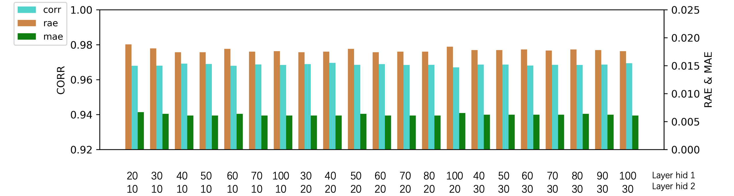
To test the parameter sensitivity of our model, we evaluate how the hidden size of the GNN component can affect the results. We report the MAE, RAE, CORR metrics on Exchange-Rate dataset. As can be seen in Figure 2, while ranging the hidden size of GNN layers from , the model performance is steady, being relatively insensitive to the hidden dimension parameter.
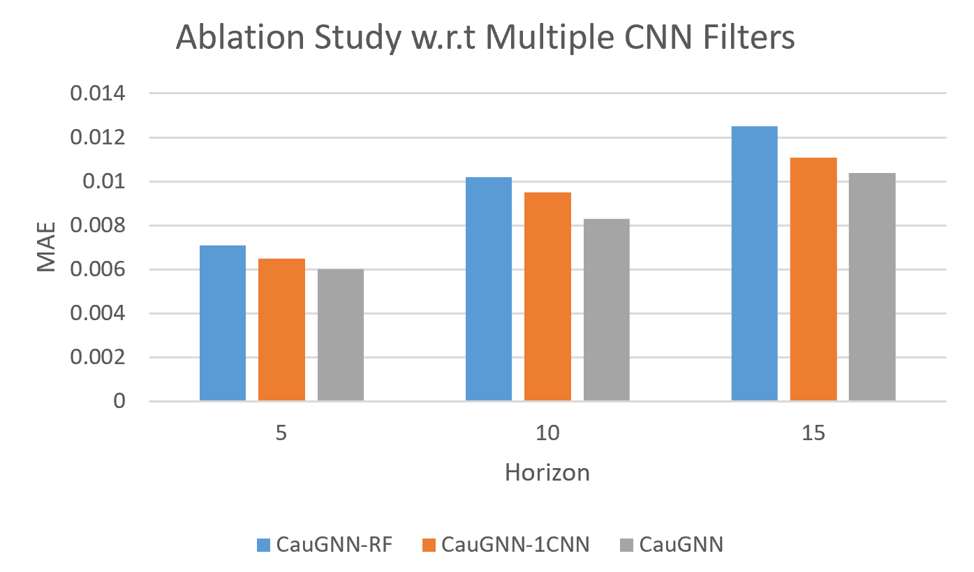
To prove the superiority of multiple CNN filters, we also did an ablation study on the Exchange-Rate dataset when horizon is 5. As shown in the Figure 3, CauGNN-RF, CauGNN-1CNN, and CauGNN respectively represent the direct use of the raw feature (original data) as the input of the node embedding model, using one CNN filter (here we set kernel size to 3), and our complete model CauGNN with three CNN filters. We can find that CauGNN-RF has the worst performance, indicating that direct use of raw feature will introduce too much noise, which is not conducive to the subsequent learning of the model; and CauGNN has the best performance, indicating that stacking multiple CNN filters can better capture multiple inherent time series period characteristics and make more accurate predictions.
5 Conclusion
In this paper, we propose a novel deep learning framework (CauGNN) for multivariate time series forecasting. Using CNN with multiple receiving fields, our model introduces causal prior information with transfer entropy features and uses graph neural network for feature extraction, which effectively improves the results in MTS forecasting. With in-depth theoretical analysis and experimental verification, we confirm that CauGNN successfully captures the causal relationship among variables and uses graph neural network to select key variables for accurate forecasting.
References
- [1] Haoyan Xu, Ziheng Duan, Yunsheng Bai, Yida Huang, Anni Ren, Qianru Yu, Qianru Zhang, Yueyang Wang, Xiaoqian Wang, Yizhou Sun, et al. Multivariate time series classification with hierarchical variational graph pooling. arXiv preprint arXiv:2010.05649, 2020.
- [2] Yishun Liu, Chunhua Yang, Keke Huang, and Weihua Gui. Non-ferrous metals price forecasting based on variational mode decomposition and lstm network. Knowledge-Based Systems, 188:105006, 2020.
- [3] Yueyang Wang, Ziheng Duan, Yida Huang, Haoyan Xu, Jie Feng, and Anni Ren. Mthetgnn: A heterogeneous graph embedding framework for multivariate time series forecasting. arXiv e-prints, pages arXiv–2008, 2020.
- [4] George EP Box, Gwilym M Jenkins, Gregory C Reinsel, and Greta M Ljung. Time series analysis: forecasting and control. John Wiley & Sons, 2015.
- [5] James D Hamilton. Time series analysis, volume 2. Princeton New Jersey, 1994.
- [6] Helmut Lütkepohl. New introduction to multiple time series analysis. Springer Science & Business Media, 2005.
- [7] Alper Tokgöz and Gözde Ünal. A rnn based time series approach for forecasting turkish electricity load. In 2018 26th Signal Processing and Communications Applications Conference (SIU), pages 1–4. IEEE, 2018.
- [8] Jeffrey L Elman. Finding structure in time. Cognitive science, 14(2):179–211, 1990.
- [9] Sepp Hochreiter and Jürgen Schmidhuber. Long short-term memory. Neural computation, 9(8):1735–1780, 1997.
- [10] Junyoung Chung, Caglar Gulcehre, KyungHyun Cho, and Yoshua Bengio. Empirical evaluation of gated recurrent neural networks on sequence modeling. arXiv preprint arXiv:1412.3555, 2014.
- [11] Guokun Lai, Wei-Cheng Chang, Yiming Yang, and Hanxiao Liu. Modeling long- and short-term temporal patterns with deep neural networks. CoRR, abs/1703.07015, 2017.
- [12] Yifu Zhou, Ziheng Duan, Haoyan Xu, Jie Feng, Anni Ren, Yueyang Wang, and Xiaoqian Wang. Parallel extraction of long-term trends and short-term fluctuation framework for multivariate time series forecasting. arXiv preprint arXiv:2008.07730, 2020.
- [13] Clive WJ Granger. Investigating causal relations by econometric models and cross-spectral methods. Econometrica: journal of the Econometric Society, pages 424–438, 1969.
- [14] Gebhard Kirchgässner, Jürgen Wolters, and Uwe Hassler. Granger causality. In Introduction to Modern Time Series Analysis, pages 95–125. Springer, 2013.
- [15] Terry Bossomaier, Lionel Barnett, Michael Harré, and Joseph T Lizier. Transfer entropy. In An introduction to transfer entropy, pages 65–95. Springer, 2016.
- [16] Thomas Dimpfl and Franziska Julia Peter. Using transfer entropy to measure information flows between financial markets. Studies in Nonlinear Dynamics & Econometrics, 17(1):85–102, 2013.
- [17] Thai Quang Tung, Taewoo Ryu, Kwang H Lee, and Doheon Lee. Inferring gene regulatory networks from microarray time series data using transfer entropy. In Twentieth IEEE International Symposium on Computer-Based Medical Systems (CBMS’07), pages 383–388. IEEE, 2007.
- [18] Margret Bauer, John W Cox, Michelle H Caveness, James J Downs, and Nina F Thornhill. Finding the direction of disturbance propagation in a chemical process using transfer entropy. IEEE transactions on control systems technology, 15(1):12–21, 2006.
- [19] Franco Scarselli, Marco Gori, Ah Chung Tsoi, Markus Hagenbuchner, and Gabriele Monfardini. The graph neural network model. IEEE Transactions on Neural Networks, 20(1):61–80, 2008.
- [20] Yueyang Wang, Ziheng Duan, Binbing Liao, Fei Wu, and Yueting Zhuang. Heterogeneous attributed network embedding with graph convolutional networks. In Proceedings of the AAAI Conference on Artificial Intelligence, volume 33, pages 10061–10062, 2019.
- [21] Ziheng Duan, Yueyang Wang, Weihao Ye, Zixuan Feng, Qilin Fan, and Xiuhua Li. Connecting latent relationships over heterogeneous attributed network for recommendation. arXiv preprint arXiv:2103.05749, 2021.
- [22] Justin Gilmer, Samuel S Schoenholz, Patrick F Riley, Oriol Vinyals, and George E Dahl. Neural message passing for quantum chemistry. In Proceedings of the 34th International Conference on Machine Learning-Volume 70, pages 1263–1272. JMLR. org, 2017.
- [23] Zhitao Ying, Jiaxuan You, Christopher Morris, Xiang Ren, Will Hamilton, and Jure Leskovec. Hierarchical graph representation learning with differentiable pooling. In Advances in neural information processing systems, pages 4800–4810, 2018.
- [24] Haoyan Xu, Runjian Chen, Yunsheng Bai, Ziheng Duan, Jie Feng, Yizhou Sun, and Wei Wang. Cosimgnn: Towards large-scale graph similarity computation. arXiv preprint arXiv:2005.07115, 2020.
- [25] Haoyan Xu, Ziheng Duan, Yueyang Wang, Jie Feng, Runjian Chen, Qianru Zhang, and Zhongbin Xu. Graph partitioning and graph neural network based hierarchical graph matching for graph similarity computation. Neurocomputing, 439:348–362, 2021.
- [26] Thomas N. Kipf and Max Welling. Semi-supervised classification with graph convolutional networks. CoRR, abs/1609.02907, 2016.
- [27] William L. Hamilton, Rex Ying, and Jure Leskovec. Inductive representation learning on large graphs. CoRR, abs/1706.02216, 2017.
- [28] Jie Chen, Tengfei Ma, and Cao Xiao. Fastgcn: fast learning with graph convolutional networks via importance sampling. arXiv preprint arXiv:1801.10247, 2018.
- [29] Keyulu Xu, Weihua Hu, Jure Leskovec, and Stefanie Jegelka. How powerful are graph neural networks? arXiv preprint arXiv:1810.00826, 2018.
- [30] Christopher Morris, Martin Ritzert, Matthias Fey, William L Hamilton, Jan Eric Lenssen, Gaurav Rattan, and Martin Grohe. Weisfeiler and leman go neural: Higher-order graph neural networks. In Proceedings of the AAAI Conference on Artificial Intelligence, volume 33, pages 4602–4609, 2019.
- [31] Petar Veličković, Guillem Cucurull, Arantxa Casanova, Adriana Romero, Pietro Lio, and Yoshua Bengio. Graph attention networks. arXiv preprint arXiv:1710.10903, 2017.
- [32] Shuang Han, Hongbin Dong, Xuyang Teng, Xiaohui Li, and Xiaowei Wang. Correlational graph attention-based long short-term memory network for multivariate time series prediction. Applied Soft Computing, 106:107377, 2021.
- [33] Thomas Schreiber. Measuring information transfer. Physical review letters, 85(2):461, 2000.
- [34] Diederik P Kingma and Jimmy Ba. Adam: A method for stochastic optimization. arXiv preprint arXiv:1412.6980, 2014.
- [35] Luis M Candanedo, Véronique Feldheim, and Dominique Deramaix. Data driven prediction models of energy use of appliances in a low-energy house. Energy and buildings, 140:81–97, 2017.
- [36] Yao Qin, Dongjin Song, Haifeng Chen, Wei Cheng, Guofei Jiang, and Garrison Cottrell. A dual-stage attention-based recurrent neural network for time series prediction. arXiv preprint arXiv:1704.02971, 2017.
- [37] Yann LeCun, Yoshua Bengio, et al. Convolutional networks for images, speech, and time series. The handbook of brain theory and neural networks, 3361(10):1995, 1995.
- [38] Ashish Vaswani, Noam Shazeer, Niki Parmar, Jakob Uszkoreit, Llion Jones, Aidan N Gomez, Ł ukasz Kaiser, and Illia Polosukhin. Attention is all you need. In I. Guyon, U. V. Luxburg, S. Bengio, H. Wallach, R. Fergus, S. Vishwanathan, and R. Garnett, editors, Advances in Neural Information Processing Systems 30, pages 5998–6008. Curran Associates, Inc., 2017.
- [39] Jiezhu Cheng, Kaizhu Huang, and Zibin Zheng. Towards better forecasting by fusing near and distant future visions. arXiv preprint arXiv:1912.05122, 2019.
[./Figure/Ziheng.jpg] Ziheng Duan received his B.E. in July, 2020 at Zhejiang University, College of Control Science and Engineering. His research interests lie in the area of Machine Learning, Computational Biology, Graph Representation Learning, Time Series Analysis, espeically the interaction of them.
{biography}
[./Figure/Haoyan.jpg] Haoyan Xu received his B.E. in July, 2020 at Zhejiang University, College of Control Science and Engineering. His research interests lie in the area of Graph Representation Learning, Time Series Analysis, Robot Learning and Microfluidics. He is particular interested in graph neural networks, with their applications in language processing, graph mining, etc.
[./Figure/Yida.jpg] Yida Huang received his B.E. in July, 2020 at Zhejiang University, College of Computer Science and Engineering. His research interests lie in the area of Time Series Analysis, Graph Representation Learning, Natural Language Processing, and their applications in Cyber Security.
[./Figure/Jiefeng.jpg] Jie Feng received his B.E. in July, 2021 at Zhejiang University, College of Control Science and Engineering, who will receive his B.S. in June. 2021. His research interests include artificial intelligence and robotics.
[./Figure/Yueyang.jpg] Yueyang Wang received the B.E. degree from the Software Institute, Nanjing University, Nanjing, China, and the Ph.D. degree from Zhejiang University, Hangzhou, China. She is currently a Lecturer with the School of Big Data and Software Engineering, Chongqing University. Her research interests include social network analysis and data mining.