Berry curvature for coupled waves of magnons and electromagnetic waves

Abstract

In this paper, we introduce Berry curvature, topological Chern number and topological chiral edge mode, that emerge from a hybridization between magnon and electromagnetic wave in a ferromagnet insulator. By focusing on the energy conservation, we first reformulate the Landau-Lifshitz-Maxwell equation into a Hermitian eigenvalue equation. From the eigenvalue equation, we define the Berry curvature of the magnon-photon coupled waves. We show that the Berry curvature thus introduced shows a prominent peak around a hybridization point between magnon mode and photon mode, and a massive hybrid mode takes a non-zero Chern number ($\pm 1$) due to the magnon-photon coupling. In accordance with the non-zero Chern number, the topological edge modes emerge inside the hybridization gap at a domain wall between two ferromagnetic insulators with opposite magnetizations.

I Introduction

Coupled waves between ferromagnetic moments and electromagnetic waves have been studied for a long time. Dispersion relations of the coupled waves of the magnon and the electromagnetic wave in layered film structures consisting of magnetic, ferroelectric, and insulating layers, are studied theoretically Demidov and Kalinikos (2000); Demidov et al. (2002a, b) and experimentally. In recent years, coupling between quantum spins and photons have attracted much attention both in theory and in experiment. The coupled wave of spins and photons behaves differently depending on the strength of the coupling. When the coupling is strong, the wave is called a magnon-polariton Mills and Burstein (1974); Lehmeyer and Merten (1985). The magnon-polariton is promising for applications in quantum information science and technology. Recently, strong coupling between the Kittel mode and the cavity mode is studied in the YIG sphere Zhang et al. (2014); Tabuchi et al. (2014, 2015), film Cao et al. (2015), and film split rings Bhoi et al. (2014).

The Berry curvature in various physical systems has also been attracting many researchers. A geometric character of the Bloch wavefunction gives rise to new phenomena such as topological electric and thermal Hall effect Xiao et al. (2010). The Berry curvature have been studied in electronsChang and Niu (1996); Sundaram and Niu (1999), photonsBliokh and Bliokh (2004); Onoda et al. (2004); Bliokh and Bliokh (2004, 2004, 2006); Onoda et al. (2006); Haldane and Raghu (2008); Raghu and Haldane (2008), magnonsOnose et al. (2010); Matsumoto and Murakami (2011a, b); Okamoto and Murakami (2017); Zhang et al. (2013); Shindou et al. (2013a, b), and so forth. Recently, calculations of finite Berry curvature are reported in various coupled systems such as systems with charge density and current couplingJin et al. (2015, ), exciton-photon couplingKarzig et al. (2015), and magnon-phonon coupling Park and Yang (2019); Zhang et al. (2019); Go et al. (2019); Park et al. (2019); Shen and Kim (2019). The hybridizations among these degrees of freedom lead to topological bands and novel edge states inside a hybridization gap. In the previous work, we have calculated the Berry curvature of magnetoelastic wave, by formulating a Hermitian eigenvalue equation from an equation of motion for the magnetoelastic waveOkamoto et al. (2020).

In this paper, we formulate a Hermitian eigenvalue equation for coupled equations of motion for ferromagnetic moments and electromagnetic waves. Based on the formulation, we calculate the Berry curvature of the coupled waves of magnons and electromagnetic wavesAkhiezer et al. (1968). We find that the Berry curvature is prominently enhanced at a crossing point of the dispersions and we carify its asymptotic behavior around the crossing point. We wind that in the presence of the finite hybridization, the topological Chern number of the coupled wave becomes quantized to be non-zero integer. We show that in accordance with the non-zero Chern number, non-trivial topological edge modes of the coupled wave appear inside the hybridization gap at a domain wall.

This paper is organized as follows. In Section II, we formulate generalized Hermitian eigenvalue equations from the equations of motion of magnons and electromagnetic waves and calculate eigenfrequencies. In Sections III and IV, we calculate the Berry curvature, the Chern number and its edge modes of the magnon and electromagnetic waves. We summarize the paper in Sec. V.

II Formulation of eigenvalue equation

We consider a three-dimensional ferromagnetic insulator with isotropic electric permittivity. The saturation magnetization ${\bm{M}_{0}}$ and the applied magnetic field ${\bm{H}_{0}}$ are parallel to each other, and they are along the $z$-direction. The magnon field is described by a magnetization ${\bm{m}}$ in the $xy$ plane (Fig. 1). We assume that electromagnetic waves with the magnetic flux density ${\bm{b}}$ and the electric field ${\bm{e}}$ trasmit entirely through the ferromagnetic insulator without dissipation. The amplitudes of the magnon and the electromagnetic waves are proportional to $\exp{i({\bm{k}\cdot r}-\omega t)}$, with frequency $\omega$ and wavevector ${\bm{k}}\equiv(k_{x},k_{y},k_{z})\equiv k(\sin\theta\cos\varphi,\sin\theta\sin\varphi,\cos\theta)$ (Fig. 1). Therefore, $\theta$ represents an angle between the wavevector and the saturation magnetization. The coupled equations of motions (EOM) consist of the Landau-Lifshitz equation and the Maxwell equation. In terms of the wavevector ${\bm{k}}$, the EOM take forms of

$$\frac{\partial{m_{x}}}{\partial t} = \frac{\omega_{M}}{4\pi}{b_{y}}-\omega_{s}{m_{y}},$$ (1)

$$\frac{\partial{m_{y}}}{\partial t} = -\frac{\omega_{M}}{4\pi}{b_{x}}+\omega_{s}{m_{x}},$$ (2)

$$\frac{\partial{\bm{b}}}{\partial t} = -icK{\bm{e}},$$ (3)

$$\frac{\partial{\bm{e}}}{\partial t} = i\frac{cK}{\epsilon}{(\bm{b}-4\pi\bm{m})},$$ (4)

where $\omega_{s}\equiv\omega_{M}+\omega_{H}$, $\omega_{M}\equiv 4\pi gM_{0}$, $\omega_{H}\equiv gH_{0}$, $g$ is gyromagnetic constant, $c$ is the speed of light, $\epsilon$ is the permittivity, and ${K}$ is an anti-symmetric matrix defined as

$$K=\left(\begin{array}[]{ccc}0&-k_{z}&k_{y}\\ k_{z}&0&-k_{x}\\ -k_{y}&k_{x}&0\end{array}\right).$$ (8)

For the later convenience, let us express Eqs. (1)-(4) as

$$i\frac{\partial}{\partial t}{\bm{x}}_{\bm{k}} = H_{\rm eff}{\bm{x}}_{\bm{k}},$$ (9)

where ${\bm{x}}_{\bm{k}}$ is the eigenvector, ${\bm{x}}_{\bm{k}}={}^{t}({m}_{\bm{k},x},{m}_{\bm{k},y},\ {\bm{b}}_{\bm{k}},\ {\bm{e}}_{\bm{k}})$. The 8 $\times$ 8 matrix $H_{\rm eff}$ is given by

$$H_{\rm eff} = \begin{pmatrix}\omega_{s}{\sigma_{2}}&-\frac{\omega_{M}}{4\pi}{\sigma^{\prime}_{2}}&{0}\\ {0}&{0}&cK\ \\ -\frac{4\pi c}{\epsilon}(K^{\prime})^{t}\ &-\frac{c}{\epsilon}K\ &{0}\\ \end{pmatrix}$$ (10)

with a 2 $\times$ 2 matrix ${\sigma_{2}}$ and 2 $\times$ 3 matrices $I^{\prime},\ {\sigma^{\prime}_{2}},\ {K^{\prime}}$:

$${I^{\prime}} = \left(\begin{array}[]{ccc}1&0&0\\ 0&1&0\\ \end{array}\right),$$ (13)

$${\sigma_{2}} = \left(\begin{array}[]{ccc}0&-i\\ i&0\\ \end{array}\right),\ \ {\sigma^{\prime}_{2}}=\left(\begin{array}[]{ccc}0&-i&0\\ i&0&0\\ \end{array}\right),$$ (18)

$${K^{\prime}} = \left(\begin{array}[]{ccc}0&-k_{z}&k_{y}\\ k_{z}&0&-k_{x}\\ \end{array}\right).$$ (21)

We call $H_{\rm eff}$ an effective Hamiltonian.

To define the Berry curvature for the coupled wave from the EOM, let us assume that a constant Hermitian matrix $\gamma$ makes $H_{\rm eff}$ to be Hermtian as $\tilde{H}_{\rm eff}\equiv\gamma H_{\rm eff}=\tilde{H}^{\dagger}_{\rm eff}$. In terms of these Hermitian matrices, the coupled EOM reduces to

$$i\gamma\frac{\partial{\bm{x}}_{\bm{k}}}{\partial t} = \tilde{H}_{\rm eff}{\bm{x}}_{\bm{k}}.$$ (22)

Define a ‘norm’ of ${\bm{x}}_{\bm{k}}$ in terms of the Hermitian matrix $\gamma$ as ${\bm{x}}_{\bm{k}}^{\dagger}\gamma{\bm{x}}_{\bm{k}}$. Since $\gamma$ and $\tilde{H}_{\rm eff}$ are both Hermitian, one see that the norm is a constant of motion, $\partial({\bm{x}}_{\bm{k}}^{\dagger}\gamma{\bm{x}}_{\bm{k}})/\partial t=0$. Physically speaking, the constant of motion must correspond to a total energy density of the system. Thus, we choose the Hermtian matrix $\gamma$ as

$$\gamma = \begin{pmatrix}\frac{(4\pi)^{2}\omega_{s}}{\omega_{M}}I&-4\pi I^{\prime}&{{0}}\\ -4\pi(I^{\prime})^{t}&I&{{0}}\\ {{0}}&{{0}}&\epsilon I\end{pmatrix},$$ (23)

with

$$\tilde{H}_{\rm eff}(\bm{k})= \gamma H_{\rm eff}(\bm{k})$$

$$= \begin{pmatrix}\frac{{(4\pi\omega_{s})}^{2}}{\omega_{M}}{\sigma_{2}}&-{4\pi}\omega_{s}{\sigma^{\prime}_{2}}&-4\pi cK^{\prime}\ \\ -{4\pi}\omega_{s}({\sigma^{\prime}_{2}})^{\dagger}&{\omega_{M}}{\Sigma_{2}}&cK&\\ -{4\pi c}(K^{\prime})^{t}&-{c}K&{\bm{0}}\\ \end{pmatrix},$$

and a 3 by 3 matrix $\Sigma_{2}$,

$${\Sigma_{2}} = \left(\begin{array}[]{ccc}0&-i&0\\ i&0&0\\ 0&0&0\\ \end{array}\right).$$ (28)

Then, the norm is equal to the total energy density, consisting of the energy density of the electric wave $u_{e}$ and that of the the magnetic wave $\ u_{m}$ Morgenthaler (1972); Buris and Stancil (1985); Fishman and Morgenthaler (1983),

$${\bm{x}}_{\bm{k}}^{\dagger}\gamma{\bm{x}}_{\bm{k}} =u_{e}+u_{m},$$ (29)

$$u_{e} ={\bm{e}}_{\bm{k}}^{\dagger}\frac{\partial(\omega\hat{\epsilon})}{\partial\omega}{\bm{e}}_{\bm{k}}=\epsilon|{\bm{e}}_{\bm{k}}|^{2},$$ (30)

$$u_{m} ={\bm{h}}_{\bm{k}}^{\dagger}\frac{\partial(\omega\hat{\mu})}{\partial\omega}{\bm{h}}_{\bm{k}}=(4\pi)^{2}\frac{\omega_{H}}{\omega_{M}}|{\bm{m}}_{\bm{k}}|^{2}+|{\bm{h}}_{\bm{k}}|^{2}.$$ (31)

Here $\hat{\epsilon}$ and $\hat{\mu}$ are an isotropic permittive tensor and permeability tensor defined by ${\bm{b}}_{\bm{k}}=\hat{\mu}{\bm{h}}_{\bm{k}}$ where ${\bm{h}}_{\bm{k}}$ represents a magnetic field. We henceforth choose a normalization condition of the eigenvector ${\bm{x}}_{\bm{k}}$ as ${\bm{x}}_{\bm{k}}^{\dagger}\gamma{\bm{x}}_{\bm{k}}=1$.

The eigenvalue equation (22) gives an equation for the dispersion relation

$$\omega^{6}-\left(2\omega_{em}^{2}+\omega_{s}^{2}\right)\omega^{4}+\omega_{em}^{2}\left(\omega_{em}^{2}+2\omega_{H}\omega_{s}+\omega_{M}\omega_{s}\sin^{2}{\theta}\right)\omega^{2}-\omega_{H}\omega_{em}^{4}\left(\omega_{H}+\omega_{M}\sin^{2}{\theta}\right)=0,$$

(32)

where $\omega_{em}=ck/\sqrt{\epsilon}$. The dispersion relation in Eq. (32) has only six solutions, while the dimension of the eigenvalue equation (9) is eight. The other two are nothing but two zero modes that correspond to unphysical gauge degrees of freedom. Namely, Eqs. (3) and (4) satisfy ${\bm{k}}\cdot{\bm{b}}=0$ and ${\bm{k}}\cdot{\bm{e}}=0$, respectively and correspondingly, Eq. (9) always has two eigenvectors that belong to the zero eigenfrequency. The six physical solutions consist of pairs of positive and negative frequencies. In the following, we only consider the case of (i) $\theta=\pi/2$ as shown in Fig. 1(i). We leave the case of (ii) $\theta=0$ in Appendix A.

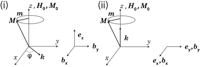
Figure 1: Schematic illustration of the magnons and the electromagnetic waves for (i) the wavevector perpendicular to the saturation magnetization ($\theta=\pi/2$) and (ii) the wavevector parallel to the saturation magnetization $\theta=0$ (in Appendix A).

III Berry curvature of coupled waves between magnons and electromagnetic waves for the case with $\theta=\pi/2$ ($k_{z}=0$)

When ${\bm{k}}$ is perpendicular to the magnetization ${M}_{0}$ ($\theta=\pi/2$), the wavevector becomes the two-dimensional vector, ${\bm{k}}=(k_{x},k_{y})=k(\cos\varphi,\sin\varphi)$, and Eq. (32) reduces to

$$\left[\omega^{4}-(\omega_{em}^{2}+\omega_{s}^{2})\omega^{2}+\omega_{em}^{2}\omega_{s}\omega_{H}\right]\left[\omega^{2}-\omega_{em}^{2}\right]=0.$$

(33)

The eigenfrequencies from the first and second parentheses correspond to the set of components $m_{x},m_{y},b_{x},b_{y},e_{z}$, and that of $b_{z},e_{x},e_{y}$, respectively. The decoupling between these two sets is due to a mirror symmetry with respect to the $xy$ plane, under which the wavevector ${\bm{k}}$ is invariant for the case with $\theta=\pi/2$. The first set comprises the hybrid waves of a magnon and an electromagnetic wave,

$$\omega^{2}_{\pm}=\frac{\omega_{s}^{2}+\omega_{em}^{2}}{2}\pm\sqrt{\left(\frac{\omega_{s}^{2}-\omega_{em}^{2}}{2}\right)^{2}+(\zeta k)^{2}}.$$ (34)

Meanwhile within the linearized EOM, the second set of the fields ($b_{z},e_{x},e_{y}$) represents a pure and is free from the hybridization with magnon with its frequency equal to $\omega_{em}$, satisfying $\omega_{-}<\omega_{em}<\omega_{+}$ (Figs. 2(a) and  3(a)). Here

$$\zeta\equiv\sqrt{\frac{\omega_{M}\omega_{s}}{\epsilon}}c$$ (35)

stands for the hybridization strength between magnon and electromagnetic waves. For the $\omega_{+}$ branch of Eq. (34), the dispersion at $k\rightarrow\infty$ and $k\rightarrow 0$ has the following asymptotic forms,

$$\omega_{+}^{2}\simeq\begin{cases}\omega^{2}_{em}+\frac{(\zeta k)^{2}}{\omega^{2}_{em}}&(k\rightarrow\infty),\\ \omega^{2}_{s}+\frac{(\zeta k)^{2}}{\omega^{2}_{s}}&(k\rightarrow 0),\end{cases}$$ (36)

and for the $\omega_{-}$ branch of Eq. (34) is

$$\omega_{-}^{2}\simeq\begin{cases}\omega^{2}_{s}-\frac{(\zeta k)^{2}}{\omega^{2}_{em}}=\omega^{2}_{mag}&(k\rightarrow\infty),\\ \omega^{2}_{em}-\frac{(\zeta k)^{2}}{\omega^{2}_{s}}&(k\rightarrow 0),\end{cases}$$ (37)

where $\omega^{2}_{mag}=\omega_{H}\omega_{s}=\omega_{H}(\omega_{H}+\omega_{M})$ is the dispersion of the magnon in the magnetostatic regime.

Let $k^{*}$ and $\tilde{\omega}$ denote the wavenumber and frequency at a crossing point between the dispersions of the magnon $\omega_{s}$ and the electromagnetic wave $\omega_{em}$ without the coupling ($\zeta=0$);

$$\omega_{s}=\omega_{em}(k^{*})\equiv\tilde{\omega},\ \ k^{*}\equiv\frac{\sqrt{\epsilon}\omega_{s}}{c}.$$ (38)

The frequencies of the coupled wave at the crossing point $k=k^{*}$ is given by

$$\omega_{\pm}=\sqrt{\tilde{\omega}^{2}\pm\tilde{\omega}\!\ \Delta\omega},\ \ \Delta\omega\equiv\frac{\zeta k^{*}}{\tilde{\omega}}.$$ (39)

where $\Delta\omega$ is defined as a hybridization gap at the crossing point. Note that the crossing point is located outside the magnetostatic regime. By using Eqs. (3)-(4), the magnetic field and the magnetization are written asStancil and Prabhakar (2009)

$${\bm{h}}_{\bm{k}}=\frac{4\pi}{1-\omega^{2}/\omega_{em}^{2}}\left(-\frac{{\bm{k}}\cdot{\bm{m}}_{\bm{k}}}{k^{2}}{\bm{k}}+\frac{\omega^{2}}{\omega_{em}^{2}}{\bm{m}}_{\bm{k}}\right),$$ (40)

$${\bm{k}}\times{\bm{h}}_{\bm{k}}=\frac{\omega^{2}/\omega_{em}^{2}}{1-\omega^{2}/\omega_{em}^{2}}{\bm{k}}\times{\bm{m}}_{\bm{k}}.$$ (41)

The magnetostatic regime is defined by $\omega\ll\omega_{em}$, where the magnetic field becomes approximately rotation free, ${\bm{h}}_{\bm{k}}\simeq-4\pi({{\bm{k}}\cdot{\bm{m}}_{\bm{k}}}){\bm{k}}/{k^{2}}$ and ${\bm{k}}\times{\bm{h}}_{\bm{k}}\simeq{\bm{0}}$. It is obvious that the crossing point ($\omega\simeq\omega_{em}$) sits far outside the magnetostatic regime. In the following, we will show that the Berry curvature of the coupled modes shows a prominent peak near the crossing point outside the magnetostatic regime.

The coupled modes between magnons and electromagnetic waves involve the components $m_{x},m_{y},b_{x},b_{y}$, and $e_{z}$. The eigenvalue equation for the coupled modes is given by a 5 $\times$ 5 matrix extracted from $\tilde{H}_{\rm eff}$:

$$\tilde{H}^{\perp}_{\rm eff}(\bm{k}){\bm{x}}_{{\bm{k}},\pm} = \omega_{\pm}\gamma^{\perp}{\bm{x}}_{{\bm{k}},\pm},$$ (42)

with

$$\tilde{H}^{\perp}_{\rm eff}(\bm{k}) = \scalebox{1.0}{$\begin{pmatrix}0&-i\frac{(4\pi)^{2}\omega_{s}^{2}}{\omega_{M}}&0&4\pi i\omega_{s}&-4\pi ck_{y}\\ i\frac{(4\pi)^{2}\omega_{s}^{2}}{\omega_{M}}&0&-4\pi i\omega_{s}&0&4\pi ck_{x}\\ 0&4\pi i\omega_{s}&0&-i\omega_{M}&ck_{y}\\ -4\pi i\omega_{s}&0&i\omega_{M}&0&-ck_{x}\\ -4\pi ck_{y}&4\pi ck_{x}&ck_{y}&-ck_{x}&0\\ \end{pmatrix}$}.$$

The energy density of the hybridized modes is given by a norm of a five-components eigenvector, ${\bm{x}}_{\bm{k}}\equiv{}^{t}(m_{{\bm{k}},x},m_{{\bm{k}},y},b_{{\bm{k}},x},b_{{\bm{k}},y},e_{{\bm{k}},z})$. The norm is given by ${\bm{x}}^{\dagger}_{\bm{k}}\gamma^{\perp}{\bm{x}}_{\bm{k}}$, where $\gamma^{\perp}$ is a 5 $\times$ 5 hermitian matrix extracted from the matrix $\gamma$: with

$$\gamma^{\perp}\equiv\begin{pmatrix}\frac{(4\pi)^{2}\omega_{s}}{\omega_{M}}&0&-4\pi&0&0\\ 0&\frac{(4\pi)^{2}\omega_{s}}{\omega_{M}}&0&-4\pi&0\\ -4\pi&0&1&0&0\\ 0&-4\pi&0&1&0\\ 0&0&0&0&\epsilon\\ \end{pmatrix}.$$ (44)

Based on this normalization, the Berry curvature of the coupled modes for the $\omega_{\pm}$ branches is defined as

$$\Omega_{z,n}(\bm{k}) = i\epsilon_{\alpha\beta}\frac{\partial\bm{x}^{\dagger}_{\bm{k},n}}{\partial k_{\alpha}}\gamma^{\perp}\frac{\partial\bm{x}_{\bm{k},n}}{\partial k_{\beta}}$$ (45)

for $n=\pm$, ${\bm{k}}=(k_{x},k_{y})=k(\cos\varphi,\sin\varphi)$, and $\alpha,\beta=x,y$ with ${\bm{x}}^{\dagger}_{{\bm{k}},n}\gamma^{\perp}{\bm{x}}_{{\bm{k}},n}=1$. Here $\epsilon_{\alpha\beta}$ is the antisymmetric tensor with $\epsilon_{xy}=-\epsilon_{yx}=1$. After a lengthy calculation, we find that the Berry curvature depends only on $k$;

$$\Omega_{z,\pm}(k)=\frac{1}{k}\frac{\partial}{\partial k}\left(\frac{\frac{\omega_{\pm}}{\omega_{s}}(\omega_{\pm}^{2}-\omega_{em}^{2})}{(2\omega_{\pm}^{2}-\omega_{s}^{2}-\omega_{em}^{2})}\right).$$ (46)

The details of the derivation are shown in Appendix B. By the similar procedure as in the magnetoelastic waveOkamoto et al. (2020), we henceforth calculate the Berry curvature in the regimes with weak and strong coupling defined by $\Delta\omega/\tilde{\omega}\ll 1$ and $\Delta\omega/\tilde{\omega}\simeq 1$, respectively.

III.1 Weak coupling regime

The weak-coupling regime between magnon and electromagnetic wave is expressed as $\omega_{M}\ll\omega_{s}$ from Eqs. (35), (38), and (39). To satisfy this condition, we set $\omega_{M}\ll\omega_{H}$ to calculate the Berry curvature. When $\omega_{M}\ll\omega_{H}$, the hybridization gap is approximately evaluate as

$$\Delta\omega\simeq\sqrt{\omega_{M}\omega_{H}}.$$ (47)

The gap is much smaller than $\tilde{\omega}$ under this condition. We show the results of the numerical calculation of the dispersion and the Berry curvature in Figs. 2 (a) and (b). The Berry curvatures for $\omega_{\pm}$ show a strong peak, and are localized at the crossing point of the dispersions.

The peak value of the Berry curvature at the crossing point ($k=k^{*}$) is approximately evaluated as

$$\Omega_{z,\pm}(k=k^{*}) = \mp\frac{\tilde{\omega}^{2}}{2{k^{*}}^{3}\zeta}=\mp\frac{1}{{2k^{*}}^{2}\Delta\omega/\tilde{\omega}}.$$ (48)

In terms of $\tilde{\omega}\simeq\omega_{H}$, and $\Delta\omega\simeq\sqrt{\omega_{M}\omega_{H}}$, we can see that the Berry curvature is proportional to $\Omega_{\pm}(k^{*})\propto{1}/{\omega_{M}^{1/2}}$ and ${1}/{\omega_{H}^{3/2}}$. The dependences of the Berry curvature on $\omega_{M}$ and $\omega_{H}$ agree with Figs. 2 (c) and (d). This result has the same form as the result of the magnetoelastic wave with respect to the hybridization gap except for some coefficientsOkamoto et al. (2020). It means that the main effect of the Berry curvature induced by the hybridization has a universal feature around the hybridization gap in the weak coupling regime.

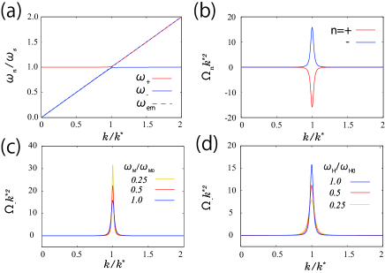
Figure 2: (Color online) Dispersions and Berry curvatures for coupled modes between magnons and electromagnetic waves in a weak coupling regime. (a) Dispersions of the $\omega_{+}$ and $\omega_{-}$ branches, and (b) Berry curvatures of the $\omega_{+}$ and $\omega_{-}$ branches as functions of $k$. The parameters are set to be $\omega_{H}/\omega_{M}=10^{3}$ with $\omega_{H}=5$ [GHz]. Berry curvatures for the $\omega_{-}$ mode is shown for (c) $\omega_{M}/\omega_{M0}=0.25,0.5,1.0$ with $\omega_{H}/\omega_{H0}=1.0$, and (d) $\omega_{H}/\omega_{H0}=\ 0.25,\ 0.5,\ 1.0$ with $\omega_{M}/\omega_{M0}=1.0$, with $\omega_{M0}=5\times 10^{-3}$ [GHz] and $\omega_{H0}=5$ [GHz].

III.2 Strong coupling regime

To calculate the Berry curvature in the strong-coupling regime, we set $\omega_{M}\simeq\omega_{s}$. The results of the dispersion and the Berry curvature are shown in Fig. 3. When the coupling between magnon and electromagnetic wave is strong, the peak of the Berry curvature at $k=k^{*}$ broadens as shown in Figs. 3 (a) and (b).

The Berry curvature of the coupled wave is affected by the hybridization even at $k\ll k^{*}$. By using Eq. (46) and the dispersions Eqs. (36) and (37), we obtain the Berry curvature for $k\ll k^{*}$

$$\Omega_{z,+}(k) \sim -\frac{\zeta^{2}}{\omega_{s}^{4}},$$ (49)

$$\Omega_{z,-}(k) \sim \frac{3\zeta^{2}c^{\prime}k}{\omega_{s}^{5}},$$ (50)

where $c^{\prime}=\sqrt{c^{2}/\epsilon-\zeta^{2}/\omega_{s}^{2}}$. These results show that the Berry curvature for $k\ll k^{*}$ is strongly affected by the coupling $\zeta$. The Berry curvature $\Omega_{z,+}$ is finite at $k\rightarrow 0$, while the Berry curvature $\Omega_{z,-}$ is zero at $k\rightarrow 0$. The analytical results agree with the result of Figs. 3 (c) and (d).

The asymptotic behavior of $\Omega_{z,-}$ around $k\simeq 0$ comes from the linearly polarized nature of the magnetic field and flux in the vicinity of $k=0$. For simplicity, we choose the wavevector ${\bm{k}}=k{\bm{e}}_{y}$ where ${\bm{e}}_{y}$ is a unit vector along the $y$-axis. A relation between $h_{x}$ and $h_{y}$ is written for the $\omega_{em}$ mode asStancil and Prabhakar (2009)

$$\frac{h_{y}}{h_{x}}=-\frac{i\omega\omega_{M}}{\omega_{mag}^{2}-\omega^{2}}.$$ (51)

Thus, the magnetic field becomes linearly polarized along the $x$ direction when $k\rightarrow 0$. In addition, the magnetic flux also becomes linearly polarized along $x$ at $k\rightarrow 0$, because the non-diagonal component of the permeability tensor $\mu_{xy}$ becomes smaller at $k\rightarrow 0$. These behaviors are the same for an arbitrary direction of ${\bm{k}}$. Thus, the eigenvector becomes asymptotically independent of $k$ and the Berry curvature $\Omega_{z,-}(k)$ becomes zero at $k\rightarrow 0$. This asymptotic behavior of the Berry curvature for the $\omega=\omega_{-}$ mode is totally different from that of the magnetoelastic wave $\omega=\omega_{+}$ in the strong coupling, where the Berry curvature of the linearly dispersive branch diverges toward $k=0$.

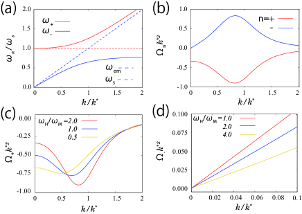
Figure 3: (Color online) Dispersions and Berry curvatures for coupled modes between magnons and electromagnetic waves in strong coupling regime (a) Dispersions of the $\omega_{+}$ and $\omega_{-}$ branches. (b) Berry curvatures of the $\omega_{+}$ and $\omega_{-}$ branches as functions of $k$. $\omega_{H}/\omega_{M}=2.0$ with $\omega_{H}=5.0$ [GHz]. The Berry curvature of the $\omega_{+}$ mode is shown for (c) $\omega_{H}/\omega_{M}=0.5,1.0,2.0$, and the $\omega_{-}$ mode for (d) $\omega_{H}/\omega_{M}=\ 0.5,\ 1/\sqrt{2},\ 1.0$.

IV Topological edge modes at $k_{z}=0$

IV.1 Chern number

Let us define an integral of the Berry curvature for the $\omega_{n}$ branch over the two-dimensional momentum space Thouless et al. (1982); Kohmoto (1985);

$${\rm Ch}_{n}=\int^{+\infty}_{-\infty}\int^{+\infty}_{-\infty}\Omega_{z,n}(\bm{k})\!\ \frac{dk_{x}dk_{y}}{2\pi},$$ (52)

with $n=\pm$. The integral is quantized to be an integer (Chern number), when the $\omega_{n}$ branch is separated from the other branches by a direct gap for any ${\bm{k}}=(k_{x},k_{y})$. The quantized integer is identical with a number of topological chiral edge modes inside the gap Halperin (1982). The edge modes are localized along a boundary of the system within the $xy$ plane. Using Eq. (46), we obtain

$${\rm Ch}_{n} = \int^{\infty}_{0}d{k}\frac{\partial}{\partial k}\left(\frac{\frac{\omega_{n}}{\omega_{s}}(\omega_{n}^{2}-\omega_{em}^{2})}{(2\omega_{n}^{2}-\omega_{s}^{2}-\omega_{em}^{2})}\right)$$ (53)

$$= N_{n}(\infty)-N_{n}(0),$$

where

$$N_{n}(k_{0})\equiv\left.\left(\frac{\frac{\omega_{n}}{\omega_{s}}(\omega_{n}^{2}-\omega_{em}^{2})}{(2\omega_{n}^{2}-\omega_{s}^{2}-\omega_{em}^{2})}\right)\right|_{k\rightarrow k_{0}}.$$ (54)

Using Eqs. (36) and (37), we have

$$N_{+}(k)=\begin{cases}0&(k\rightarrow\infty)\\ 1&(k\rightarrow 0)\end{cases},$$ (55)

and

$$N_{-}(k)=\begin{cases}\frac{\omega_{mag}}{\omega_{s}}&(k\rightarrow\infty)\\ 0&(k\rightarrow 0)\end{cases}.$$ (56)

Thus, the Chern number for the $\omega_{+}$ branch is $-1$,

$${\rm Ch}_{+}=-1.$$ (57)

The dispersion and its Chern number are illustrated in Fig. 4 (a). From the quantization of the Chern number, we expect that a chiral edge mode with $k_{z}=0$ appears inside the hybridization gap between the $\omega_{+}$ branch and $\omega_{-}$ branch.

The integral of the Berry curvature for the $\omega_{-}$ branch is not quantized to an integer. This is because the $\omega_{-}$ branch in the particle space ($\omega=\omega_{-}\geq 0$) and its hole counterpart ($\omega=-\omega_{-}\leq 0$) forms a band touching at $k=0$; $\omega_{-}(k=0)=0$. In the eigenvalue equation (9), the branch with the positive frequency and that with the negative frequency are coupled with each other. Due to the band touching at $k=0$, the Chern number for the $\omega_{-}$ branch is not well defined. As a result, the sum of the Chern number over the branches with the positive frequency region is not zero either, unlike the cases with a gap between the positive $\omega$ and the negative $\omega$ branchesShindou et al. (2013b).

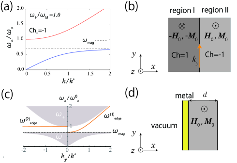
Figure 4: (Color online) Topological Chern number and topological edge modes of coupled waves between magnons and electromagnetic waves (a) Dispersions of the $\omega_{+}$ and $\omega_{-}$ branches with the Chern number for the $\omega_{+}$ branch. (b) Schematic picture of two ferromagnetic regions with opposite magnetization and magnetic field. In region I, the Chern number of the $\omega_{+}$ branch is $+1$ with ${\bm{H}}=(0,0,-H_{0})$, and in region II it is $-1$ with ${\bm{H}}=(0,0,H_{0})$. The boundary between the two regions is parallel to the $y$-axis. We define the surface momentum along $y$ as $k_{y}$. (c) Dispersions for the edge modes (orange lines) with $\omega^{0}_{H}=\omega^{0}_{M}=5.0$ [GHz]. Gray-colored regions show projections of the dispersions of the bulk modes $\omega_{+}$ and $\omega_{-}$ onto the surface momentum $k_{y}$. (d) Ferromagnetic insulator slab with a metalized surface. A chiral mode appears only in the $k_{y}<0$ on the metalized surface.

IV.2 Chiral edge modes

From the quantization of the Chern number of the $\omega_{+}$ branch, we expect that a chiral edge mode with $k_{z}=0$ appear inside the hybridization gap. The mode is localized at a boundary between topologically different regions. Here, we show an emergence of such topological chiral edge modes at an interface between two regions with opposite magnetizations. We consider a domain wall as schematically illustrated in Fig. 4 (b). The magnetization and magnetic field is directed along $-z$ direction in region I ($x<0$) and $+z$ direction in region II ($x>0$). Namely, ${\bm{H}}=(0,0,H_{0})$, ${\bm{M}}=(0,0,M_{0})$ in region II and ${\bm{H}}=(0,0,-H_{0})$, ${\bm{M}}=(0,0,-M_{0})$ in region I, where $H_{0}$ and $M_{0}$ are positive. This means $\omega_{H}=\omega^{0}_{H}\equiv gH_{0}$, $\omega_{M}=\omega^{0}_{M}\equiv 4\pi gM_{0}$, and $\omega_{s}=\omega^{0}_{s}\equiv\omega^{0}_{H}+\omega^{0}_{M}$ in region II and $\omega_{H}=-\omega^{0}_{H}$, $\omega_{M}=-\omega^{0}_{M}$, and $\omega_{s}=-\omega^{0}_{s}$ in region I. From Eq. (46), the Berry curvature for the $\omega_{n}$ branch changes its sign from the region I to the region II. Thus, the Chern number for the $\omega_{+}$ branch in the region I is $+1$, while that in the region II is $-1$.

The number of chiral edge modes at an interface with two regions with different Chern numbers equals to the difference of the two Chern numbers between the two regionsHalperin (1982). It is independent of the details of the interface. Since the Chern number in the region I and in the region II are $1$ and $-1$ respectively, two chiral edge modes are expected to emerge at the interface. To see them, we note that the wavenumber $k_{y}$ along the edge ($y$ axis) is conserved, while we should replace $k_{x}$ by $-i\partial_{x}$ in Eq. (LABEL:Hamiltonian1). We then calculate eigenmodes of Eq. (42) at the boundary. The eigenmodes localized at the boundary is proportional to $e^{ik_{y}y+\kappa x}$ for $x<0$ and $e^{ik_{y}y-\kappa x}$ for $x>0$ with $\kappa>0$. From the boundary conditions for the electromagnetic waves $b_{x}$, $h_{y}$ and $e_{z}$, we obtain two edge-mode solutions $\omega=\omega^{(1)}_{\rm edge},\ \omega^{(2)}_{\rm edge}$ inside the gap between $\omega_{+}$ and $\omega_{-}$ (see Appendix E), and their dispersion relations are shown in Fig. 4 (c). The dispersions of the edge modes are written as

$$(\omega^{(1)}_{\rm edge})^{2}=\frac{\omega_{mag}^{2}+\omega_{em}^{2}}{2}+\sqrt{\left(\frac{\omega_{mag}^{2}+\omega_{em}^{2}}{2}\right)^{2}-\omega_{H}^{2}\omega_{em}^{2}}$$

$$(k_{y}>0),\ \ \ \ \ \$$ (58)

$$\omega^{(2)}_{\rm edge}=\omega^{0}_{s}\ \ (k_{y}<0),$$ (59)

with $\omega_{em}=ck_{y}/\sqrt{\epsilon}$ and $k_{y}>0$. The dispersion $\omega^{(1)}_{\rm edge}$ touches at $k_{y}=0$ the top of the $\omega_{-}$ branch of the bulk mode. The dispersion quadratically increases in small $k_{y}$ for $k_{y}\sim k^{*}$ due to the magnon, while it linearly increases for $k_{y}\gg k^{*}$ because the electromagnetic wave is dominant. The other edge mode $\omega^{(2)}_{\rm edge}$ shows a flat dispersion as in Fig. 4 (c) with $k_{y}<0$.

An edge mode with a flat dispersion similar to Eq. (59) was also reported in a previous study of topological edge magnetoplasmonJin et al. (2015). The magnetoplasmon is a coupled wave between the charge density and electric current density in a two-dimensional electron gas (2DEG) under a high magnetic field. The previous studyJin et al. (2015) found two distinct edge modes in the 2DEG under the magnetic field, one edge mode with a flat dispersion and the other edge mode with a linear (chiral) dispersion. The edge mode with the flat dispersion carries only the electric current component, while the other edge mode carries both charge density and current components. Similarly to the topological magnetoedgeplasmon, the edge mode with the flat dispersion in the present system, Eq. (59), carries only the magnetization and the magnetic field components, but not the electric field component (see Appendix E). Meanwhile, the edge mode with the chiral dispersion, Eq. (58), is a coupled mode among magnetization, magnetic field and electric field (see Appendix E1).

The edge mode with the flat dispersion in Eq. (59) can be regarded as the Damon-Eshbach surface mode in a ferromagnetic insulator slab with its surface being metalizedSeshadri (1970). A dispersion of the surface mode of the surface-metalized ferromagnetic insulator slab with a finite thickness $d$ exists only in the $k_{y}<0$ region in Fig. 4 (d). When the thickness becomes much larger than the wavelength ($|k_{y}d|\gg 1$), the dispersion becomes flat when the exchange interaction is neglectedSeshadri (1970) and the saturated dispersion equals to Eq. (59). Note also that the boundary condition for the magnetic flux in the edge mode with the flat dispersion $\omega=\omega^{0}_{s}$ (see Appendix E) is the same as that in the surface-metalized ferromagnet, where the magnetic flux density along $x$ direction at the surface is zero due to the metalized surfaceSeshadri (1970).

V Conclusion

In this paper, we discuss the Berry curvature and topological edge modes that emerge from a hybridization between a magnon and an electromagnetic wave in a ferromagnetic insulator. By introducing a norm of eigenvector for the coupled wave based on the energy conservation, we reformulated the Landau-Lifshitz-Maxwell equation into a Hermitian eigenvalue equation. From the eigenvalue equation, we introduced the Berry curvature of the coupled waves between the magnon and the electromagnetic wave. When the wavevector of the coupled wave ${\bm{k}}$ is perpendicular to the magnetic field and magnetization, we found that the Berry curvature shows a prominent peak around a hybridization point between the magnon and the electromagnetic modes. The hybridization leads to two relevant hybrid modes; one is a magnon-like massive mode $(\omega=\omega_{+})$ at ${\bm{k}}=0$ and the other is a photon-like massless mode $(\omega=\omega_{-})$ at ${\bm{k}}=0$. Around ${\bm{k}}\simeq 0$, the Berry curvature for the massless mode converges to zero, while that for the massive mode converges to a non-zero value. We found that the Chern number for the massive mode takes a non-zero integer ($\pm 1$), and consequently two chiral edge modes emerge inside the hybridization gap at a domain wall between two ferromagnetic insulators with opposite magnetizations. One of the two edge modes carries both a magnon and an electromagnetic wave, while the other edge mode is purely magnetic and can be regarded as the Damon-Eschbach surface chiral mode of the surface-metalized ferromagnetic insulator slab.

Recently, the surface mode of the ferromagnet film in the dipole-exchange regime immune to backscattering is reportedMohseni et al. (2019). Our work provides an insight for the search of the chiral edge modes and stimulates future simulational and experimental studies on coupled waves between magnons and electromagnetic waves.

Appendix A Dispersion of the coupled wave between the magnon and the electromagnetic wave with the wavevector parallel to the magnetization

In the main text, we consider the case with ${\bm{k}}\perp{\bm{M}}_{0}$. In this Appendix, we calculate the dispersion relation for the other case, the case with ${\bm{k}}\parallel{\bm{M}}_{0}$. From Eq. (32), the dispersion relation reduces to

$$\left[\omega\left(\omega^{2}-\omega_{em}^{2}\right)-\left(\omega_{s}\omega^{2}-\omega_{H}\omega_{em}^{2}\right)\right]$$

$$\times\left[\omega\left(\omega^{2}-\omega_{em}^{2}\right)+\omega_{s}\omega^{2}-\omega_{H}\omega_{em}^{2}\right]=0.$$ (60)

From this, we obtain the dispersion relations for three branches shown in Ref. Stancil and Prabhakar, 2009. Let $\omega_{i}$ ($i=1,2,3$) be the eigenfrequencies of the waves with $0<\!\ \omega_{1}<\omega_{2}<\omega_{3}$. Among the three modes with positive frequencies, one is massive at $k=0$, $\omega(k=0)\not=0$, while the other two is massless at $k=0$. The dispersions of the massless modes take the following asymptotic forms around $k=0$,

$$\omega_{1}\approx\omega_{em}\sqrt{\frac{\omega_{H}}{\omega_{s}}}-\frac{\omega_{M}\omega_{em}^{2}}{2\omega_{s}^{2}},$$ (61)

and

$$\omega_{2}\approx\omega_{em}\sqrt{\frac{\omega_{H}}{\omega_{s}}}+\frac{\omega_{M}\omega_{em}^{2}}{2\omega_{s}^{2}}.$$ (62)

The dispersion of the massive mode has the following asymptotic form near $k=0$,

$$\omega_{3}\approx\omega_{s}+\frac{\omega_{M}\omega_{em}^{2}}{\omega_{s}^{2}}.$$ (63)

Appendix B Calculation of the Berry curvature of the coupled wave between the magnon and the electromagnetic wave

In this Appendix, we give a detailed calculation of the Berry curvature for the coupled modes between a magnon and an electromagnetic wave for the case with ${\bm{k}}\perp{\bm{M}}_{0}$. Let ${\bm{M}}_{0}$ to be along the $z$ axis. The two relevant branches with $\omega=\omega_{\pm}$ represent hybridized waves of $m_{x}$, $m_{y}$, $b_{x}$, $b_{y}$ and $e_{z}$. The eigenvalue equation for these five components, ${\bm{x}}_{\bm{k}}\equiv{}^{t}(m_{{\bm{k}},x},m_{{\bm{k}},y},b_{{\bm{k}},x},b_{{\bm{k}},y},e_{{\bm{k}},z})$, is given by:

$$\tilde{H}^{\perp}_{\rm eff}(k,\varphi){\bm{x}}_{\bm{k}} = \omega\gamma^{\perp}{\bm{x}}_{\bm{k}},$$ (64)

where

$$\tilde{H}^{\perp}_{\rm eff}(k,\varphi)=\gamma^{\perp}H_{\rm eff}(k,\varphi)$$

$$=\scalebox{1.0}{$\begin{pmatrix}0&-i\frac{(4\pi)^{2}\omega_{s}^{2}}{\omega_{M}}&0&4\pi i\omega_{s}&-4\pi ck_{y}\\ i\frac{(4\pi)^{2}\omega_{s}^{2}}{\omega_{M}}&0&-4\pi i\omega_{s}&0&4\pi ck_{x}\\ 0&4\pi i\omega_{s}&0&-i\omega_{M}&ck_{y}\\ -4\pi i\omega_{s}&0&i\omega_{M}&0&-ck_{x}\\ -4\pi ck_{y}&4\pi ck_{x}&ck_{y}&-ck_{x}&0\\ \end{pmatrix}$}.$$

(65)

Here ${\bm{k}}\equiv k(\cos{\varphi},\ \sin{\varphi})$ is within the $xy$ plane, with $\varphi$ being the angle between the $x$ axis (see Fig. 1). The norm of the eigenvector is defined through the Hermitian matrix $\gamma^{\perp}$;

$$\gamma^{\perp}=\begin{pmatrix}\frac{(4\pi)^{2}\omega_{s}}{\omega_{M}}&0&-4\pi&0&0\\ 0&\frac{(4\pi)^{2}\omega_{s}}{\omega_{M}}&0&-4\pi&0\\ -4\pi&0&1&0&0\\ 0&-4\pi&0&1&0\\ 0&0&0&0&\epsilon\\ \end{pmatrix}.$$ (66)

From the O(2) rotational symmetry in the Landau-Lifshitz-Maxwell equation, the eigenvector at finite $\varphi$ is related with that at $\varphi=0$ by the O(2) transformation,

$$\tilde{H}^{\perp}_{\rm eff}(k,\varphi=0)\tilde{\bm{x}}_{k}={\omega}\gamma^{\perp}\tilde{\bm{x}}_{k},$$ (67)

$$\bm{x}_{\bm{k}}=\begin{pmatrix}{\bm{U}}_{2}(\varphi)&&\\ &{\bm{U}}_{2}(\varphi)&\\ &&1\\ \end{pmatrix}\tilde{\bm{x}}_{k},$$ (68)

where

$${\bm{U}}_{2}(\varphi)=\begin{pmatrix}\cos\varphi&-\sin\varphi\\ \sin\varphi&\cos\varphi\\ \end{pmatrix}.$$ (69)

The dependence on $\varphi$ and $k$ in ${\bm{x}}_{\bm{k}}$ is now factorized into ${\bm{U}}_{2}(\varphi)$ and $\tilde{\bm{x}}_{k}$. $\tilde{\bm{x}}_{k}$ is an eigenstate of the following Hermitian matrix,

$$\tilde{H}^{\perp}_{\rm eff}(k,\varphi=0)$$

$$=\begin{pmatrix}0&-i\frac{(4\pi)^{2}\omega_{s}^{2}}{\omega_{M}}&0&4\pi i\omega_{s}&0\\ i\frac{(4\pi)^{2}\omega_{s}^{2}}{\omega_{M}}&0&-4\pi i\omega_{s}&0&4\pi ck\\ 0&4\pi i\omega_{s}&0&-i\omega_{M}&0\\ -4\pi i\omega_{s}&0&i\omega_{M}&0&-ck\\ 0&4\pi ck&0&-ck&0\\ \end{pmatrix}.$$

By using the factorized form for ${\bm{x}}_{\bm{k}}$ , the Berry curvature is calculated as

$$\Omega_{z,n}(\bm{k}) = i\epsilon_{\alpha\beta}\frac{\partial\bm{x}^{\dagger}_{\bm{k}}}{\partial k_{\alpha}}\gamma^{\perp}\frac{\partial\bm{x}_{\bm{k}}}{\partial k_{\beta}}$$ (71)

$$= \frac{1}{k}\frac{\partial}{\partial k}\Big{(}\tilde{\bm{x}}^{\dagger}_{k}\Gamma\tilde{\bm{x}}_{k}\Big{)},$$

$$\Gamma = \begin{pmatrix}0&-\frac{(4\pi)^{2}\omega_{s}}{\omega_{M}}&0&4\pi&0\\ \frac{(4\pi)^{2}\omega_{s}}{\omega_{M}}&0&-4\pi&0&0\\ 0&4\pi&0&-1&0\\ -4\pi&0&1&0&0\\ 0&0&0&0&0\end{pmatrix},$$ (72)

with the normalization condition $\tilde{\bm{x}}^{\dagger}_{k}\gamma^{\perp}\tilde{\bm{x}}_{k}=1$. To evaluate Eq. (71), it is convenient to introduce an unnormalized eigenstate $\tilde{\bm{X}}_{k}$, which is related with $\tilde{\bm{x}}_{k}$ by

$$\tilde{\bm{x}}_{k}\equiv\frac{\tilde{\bm{X}}_{k}}{\sqrt{\tilde{\bm{X}}^{\dagger}_{k}\gamma^{\perp}\tilde{\bm{X}}_{k}}}.$$ (73)

In terms of the unnormalized eigenstate, the Berry curvature is given by

$$\Omega_{z,n}(\bm{k})=\frac{1}{k}\frac{\partial}{\partial k}\left(\frac{\tilde{\bm{X}}_{k}\Gamma\tilde{\bm{X}}_{k}}{\tilde{\bm{X}}_{k}\gamma^{\perp}\tilde{\bm{X}}_{k}}\right).$$ (74)

From the Hermitian eigenvalue equation, the eigenstate satisfies

$$\begin{pmatrix}-\frac{(4\pi)^{2}\omega_{s}\omega}{\omega_{M}}&-i\frac{(4\pi)^{2}\omega_{s}^{2}}{\omega_{M}}&4\pi\omega&4\pi i\omega_{s}&0\\ i\frac{(4\pi)^{2}\omega_{s}^{2}}{\omega_{M}}&-\frac{(4\pi)^{2}\omega_{s}\omega}{\omega_{M}}&-4\pi i\omega_{s}&4\pi\omega&4\pi ck\\ 4\pi\omega&4\pi i\omega_{s}&-\omega&-i\omega_{M}&0\\ -4\pi i\omega_{s}&4\pi\omega&i\omega_{M}&-\omega&-ck\\ 0&4\pi ck&0&-ck&-\epsilon\omega\\ \end{pmatrix}\tilde{\bm{X}}_{k}={\bm{0}}.$$

Thus, we have

$$\tilde{\bm{X}}_{k}=\begin{pmatrix}-i\frac{\omega_{M}ck}{4\pi(\omega^{2}-\omega_{s}^{2})}\\ \frac{\omega_{s}\omega_{M}ck}{4\pi\omega(\omega^{2}-\omega_{s}^{2})}\\ 0\\ -\frac{ck}{\omega}\\ 1\end{pmatrix}.$$ (76)

By using this wavefuntion and Eq. (74), we obtain the Berry curvature for the two eigenmodes with $\omega=\omega_{\pm}$:

$$\Omega_{z,\pm}(k)=\frac{1}{k}\frac{\partial}{\partial k}\left(\frac{\frac{\omega_{\pm}}{\omega_{s}}(\omega_{\pm}^{2}-\omega_{em}^{2})}{(2\omega_{\pm}^{2}-\omega_{s}^{2}-\omega_{em}^{2})}\right).$$ (77)

Appendix C Wavenumber and Berry curvature at the crossing point of the dispersions for the electromagnetic wave and the magnon

Here we present a detailed calculation of the peak value of the Berry curvature at the crossing point between magnon and photon mode. The wavevector at the crossing point $k^{*}$ is defined by

$$k^{*}=\sqrt{\frac{\epsilon}{c^{2}}}(\omega_{H}+\omega_{M}).$$ (78)

The dispersion and the Berry curvature around $k=k^{*}$ are given by

$${\omega}_{\pm}\simeq \sqrt{\frac{c^{2}(k^{2}+{k^{*}}^{2})}{2\epsilon}}$$

$$\times\left(1\pm\frac{1}{(k^{2}+{k^{*}}^{2})}\sqrt{\frac{(k^{2}-{k^{*}}^{2})^{2}}{4}+\left(\frac{\epsilon\zeta k}{c^{2}}\right)^{2}}\right).$$ (79)

Using Eqs. (77, 79), we obtain peak values of the Berry curvature;

$$\Omega_{z,\pm}(k=k^{*}) = \mp\frac{\tilde{\omega}^{2}}{2{k^{*}}^{3}\zeta}=\mp\frac{1}{{2k^{*}}^{2}\Delta\omega/\tilde{\omega}}.$$ (80)

Appendix D Hermitian eigenvalue problems in the other bases

In the main text, we use the basis for the eigenvector as ${\bm{x}}_{{\bm{k}},1}\equiv({\bm{m}}_{\bm{k}},{\bm{b}}_{\bm{k}},{\bm{e}}_{\bm{k}})^{t}$. Using ${\bm{b}}_{\bm{k}}={\bm{h}}_{\bm{k}}+4\pi{\bm{m}}_{\bm{k}}$, one can change the basis for the eigenvector into either ${\bm{x}}_{{\bm{k}},2}\equiv({\bm{m}}_{\bm{k}},{\bm{h}}_{\bm{k}},{\bm{e}}_{\bm{k}})^{t}$ or ${\bm{x}}_{{\bm{k}},3}\equiv({\bm{b}}_{\bm{k}},{\bm{h}}_{\bm{k}},{\bm{e}}_{\bm{k}})^{t}$. In terms of ${\bm{x}}_{{\bm{k}},2}$, the Hermitian Hamiltonian in the eigenvalume problem changes into

$$H_{2}({\bm{k}}) = \scalebox{1.0}{$\begin{pmatrix}0&-i\frac{(4\pi)^{2}\omega_{H}^{2}}{\omega_{M}}&0&4\pi i\omega_{H}&0\\ i\frac{(4\pi)^{2}\omega_{H}^{2}}{\omega_{M}}&0&-4\pi i\omega_{H}&0&0\\ 0&4\pi i\omega_{H}&0&-i\omega_{M}&ck_{y}\\ -4\pi i\omega_{H}&0&i\omega_{M}&0&-ck_{x}\\ 0&0&ck_{y}&-ck_{x}&0\\ \end{pmatrix}$}.$$

In the new basis, a norm of the eigenvectors should be redefined as $\left<{\bm{x}}_{{\bm{k}},2}\right|\gamma_{2}\left|{\bm{x}}_{{\bm{k}},2}\right>$ with

$$\gamma_{2}=\begin{pmatrix}\frac{(4\pi)^{2}\omega_{H}}{\omega_{M}}&0&0&0&0\\ 0&\frac{(4\pi)^{2}\omega_{H}}{\omega_{M}}&0&0&0\\ 0&0&1&0&0\\ 0&0&0&1&0\\ 0&0&0&0&\epsilon\\ \end{pmatrix}.$$ (82)

(compare this with Eqs. (29), (30), and (31). We can also choose another basis, ${\bm{x}}_{{\bm{k}},3}\equiv({\bm{b}}_{\bm{k}},{\bm{h}}_{\bm{k}},{\bm{e}}_{\bm{k}})^{t}$, with

$$H_{3}({\bm{k}}) = \scalebox{1.0}{$\begin{pmatrix}0&-i\frac{\omega_{H}^{2}}{\omega_{M}}&0&i\frac{\omega_{H}\omega_{s}}{\omega_{M}}&0\\ i\frac{\omega_{H}^{2}}{\omega_{M}}&0&-i\frac{\omega_{H}\omega_{s}}{\omega_{M}}&0&0\\ 0&i\frac{\omega_{H}\omega_{s}}{\omega_{M}}&0&-i\frac{\omega_{s}^{2}}{\omega_{M}}&ck_{y}\\ -i\frac{\omega_{H}\omega_{s}}{\omega_{M}}&0&i\frac{\omega_{s}^{2}}{\omega_{M}}&0&-ck_{x}\\ 0&0&ck_{y}&-ck_{x}&0\\ \end{pmatrix}$},$$

and

$$\gamma_{3}=\begin{pmatrix}\frac{\omega_{H}}{\omega_{M}}&0&-\frac{\omega_{H}}{\omega_{M}}&0&0\\ 0&\frac{\omega_{H}}{\omega_{M}}&0&-\frac{\omega_{H}}{\omega_{M}}&0\\ -\frac{\omega_{H}}{\omega_{M}}&0&\frac{\omega_{s}}{\omega_{M}}&0&0\\ 0&-\frac{\omega_{H}}{\omega_{M}}&0&\frac{\omega_{s}}{\omega_{M}}&0\\ 0&0&0&0&\epsilon\\ \end{pmatrix}.$$ (84)

The norm in this basis is defined as $\left<{\bm{x}}_{{\bm{k}},3}\right|\gamma_{3}\left|{\bm{x}}_{{\bm{k}},3}\right>$. In accordance with the change of the norm, the Berry curvature in these new bases are defined by Eq. (45) with a replacement of $\gamma^{\perp}$ and ${\bm{x}}_{{\bm{k}}}$ by $\gamma_{2}$ and ${\bm{x}}_{{\bm{k}},2}$ or by $\gamma_{3}$ and ${\bm{x}}_{{\bm{k}},3}$ respectively. It is important to note that these different formulae give the same calculation result of the Berry curvature as Eq. (46).

Appendix E Calculation of the edge-mode solutions of the coupled wave between the magnon and the electromagentic wave

In the main text, we discuss the emergence of the chiral edge modes at the boundary between the two ferromagnetic regions with an opposite magnetization and magnetic field. In the following, we will give a detailed derivation of the edge modes and their dispersions. From Eq. (33) with the replacement of $k_{x}$ by $\pm i\kappa\ (\kappa>0)$, the eigenfrequencies of the edge modes shold satisfy the following equation;

$$\omega^{4}-(\tilde{\omega}^{2}_{em}+\omega^{2}_{s}) \omega^{2}+\tilde{\omega}^{2}_{em}\omega^{2}_{mag}=0,$$ (85)

$$\tilde{\omega}^{2}_{em} \equiv\frac{c^{2}(k_{y}^{2}-\kappa^{2})}{\epsilon}.$$ (86)

Unnormalized eigenvectors for the edge modes are obtained from Eqs. (76) and (68) with the replacement of $k_{x}$ by $+i\kappa\ (\kappa>0)$ for the region II ($x>0$) and by $-i\kappa$ for the region I ($x<0$), Eqs. (76) and (68) give the unnormalized eigenvectors at the both sides of the boundary,

$$\psi_{k_{y}}(x,y)=$$

$$\begin{pmatrix}m_{x,k_{y}}\\ m_{y,k_{y}}\\ b_{x,k_{y}}\\ b_{y,k_{y}}\\ e_{z,k_{y}}\\ \end{pmatrix}=C_{\pm}\begin{pmatrix}\pm\frac{\omega_{M}\!\ c\kappa}{4\pi}-\frac{\omega_{s}\omega_{M}ck_{y}}{4\pi\omega}\\ -i\frac{\omega_{M}\!\ ck_{y}}{4\pi}\pm i\frac{\omega_{s}\omega_{M}c\kappa}{4\pi\omega}\\ \frac{ck_{y}}{\omega}(\omega^{2}-\omega_{s}^{2})\\ \mp i\frac{c\kappa}{\omega}(\omega^{2}-\omega_{s}^{2})\\ (\omega^{2}-\omega_{s}^{2})\end{pmatrix}e^{\mp\kappa x+ik_{y}y},$$

$$\ \ \ \ \ \ \ \ \ \ \ \ \ \ \ \ \ \ \ \ \ \ \ \ \ \ \ \ \ \ \ \ \ \ \ \ \ \ \ \ \ \ \ \ \ \ \ (x>0\ (x<0))$$ (87)

where $C_{\pm}$ are constants. Here, we note that $\omega_{H}=\omega^{0}_{H}\equiv gH_{0}$, $\omega_{M}=\omega^{0}_{M}\equiv 4\pi gM_{0}$, and $\omega_{s}=\omega^{0}_{s}\equiv\omega^{0}_{H}+\omega^{0}_{M}$ for $x>0$ and $\omega_{H}=-\omega^{0}_{H}$, $\omega_{M}=-\omega^{0}_{M}$, and $\omega_{s}=-\omega^{0}_{s}$ for $x<0$. Next, we need to determine the constant factors $C_{\pm}$ so as to satisfy the appropriate boundary conditions:

$$b_{x}(x=0+) = b_{x}(x=0-),$$ (88)

$$e_{z}(x=0+) = e_{z}(x=0-),$$ (89)

$$h_{y}(x=0+) = h_{y}(x=0-).$$ (90)

In the following, to calculate edge-modes solutions, we study cases the $\omega\neq\omega^{0}_{s}$ and $\omega=\omega^{0}_{s}$ separately.

E.1 edge-mode solution with $\omega\neq\omega^{0}_{s}$

Let us first consider an edge-mode solution with $\omega\neq\omega^{0}_{s}$. From Eq. (87), to satisfy the boundary conditions for $b_{x}$ and $e_{z}$ at $x=0$ we need to set $C_{+}=C_{-}$. Then the boundary condition for $h_{y}$ at $x=0$ gives a relation between $\kappa$ and $k_{y}$,

$$\kappa=\frac{\omega^{0}_{M}\!\ \omega}{\omega^{2}-\omega^{2}_{mag}}k_{y}.$$ (91)

A substitution of Eq. (91) into Eqs. (85) and (86) leads to the dispersion relation between $k_{y}$ and $\omega$ for localized modes:

$$\omega^{4}-(\omega^{2}_{mag}+\omega^{2}_{em})\omega^{2}+\omega^{2}_{H}\omega^{2}_{em}=0,$$ (92)

with $\omega_{em}\equiv ck_{y}/\sqrt{\epsilon}$ for $\omega\neq\omega_{mag}$. It gives the chiral dispersion, Eq. (58), where $k_{y}>0$ is required by the positiveness of $\kappa$.

The edge mode with the chiral dispersion involves both a magnetization and an electric field. For $k_{y}\rightarrow 0$, the chiral edge mode becomes magnonic,

$$\begin{pmatrix}m_{x,k_{y}}(x,y)\\ m_{y,k_{y}}(x,y)\\ b_{x,k_{y}}(x,y)\\ b_{y,k_{y}}(x,y)\\ e_{z,k_{y}}(x,y)\\ \end{pmatrix}=C_{\pm}\begin{pmatrix}\frac{1}{4\pi\sqrt{2}}\sqrt{\frac{\omega_{M}}{\omega_{s}}}\\ \mp\frac{i}{4\pi\sqrt{2}}\sqrt{\frac{\omega_{M}}{\omega_{H}}}\\ 0\\ \mp\frac{i}{\sqrt{2}}\sqrt{\frac{\omega_{M}}{\omega_{H}}}\\ 0\end{pmatrix}\!\ e^{\mp\kappa x+ik_{y}y},$$

$$(x>0\ (x<0)).$$ (93)

For $k_{y}\gg k^{*}$, the chiral mode becomes photonic,

$$\begin{pmatrix}m_{x,k_{y}}(x,y)\\ m_{y,k_{y}}(x,y)\\ b_{x,k_{y}}(x,y)\\ b_{y,k_{y}}(x,y)\\ e_{z,k_{y}}(x,y)\\ \end{pmatrix}=C_{\pm}\begin{pmatrix}0\\ 0\\ 1/\sqrt{2}\\ 0\\ 1/\sqrt{2\epsilon}\end{pmatrix}\!\ e^{\mp\kappa x+ik_{y}y},$$

$$(x>0\ (x<0)).$$ (94)

E.2 edge-mode solution with $\omega=\omega^{0}_{s}$

First, Eq. (87) satisfies the boundary conditions for $b_{x}$ and $e_{z}$, while the boundary condition for $h_{y}$ is satisfied by setting $C_{-}=-C_{+}$. Then, by combining $\omega=\omega^{0}_{s}$, we obtain with Eqs. (85) and (86) relates $k_{y}$ with $\kappa$ as,

$$\tilde{\omega}^{2}_{em}\equiv\frac{c^{2}(k_{y}^{2}-\kappa^{2})}{\epsilon}=0,\ \ \Rightarrow k_{y}=\pm\kappa$$ (95)

A case with $k_{y}=+\kappa\!\ (>0)$ makes all the components in Eq. (87) to be zero, giving no physical solution. The other case with $k_{y}=-\kappa\!\ (<0)$ gives a physical edge-mode solution with the flat dispersion, Eq. (59). From Eq. (87), the edge mode with the flat dispersion involves only the magnetization and the magnetic field;

$$\begin{pmatrix}m_{x,k_{y}}(x,y)\\ m_{y,k_{y}}(x,y)\\ b_{x,k_{y}}(x,y)\\ b_{y,k_{y}}(x,y)\\ e_{z,k_{y}}(x,y)\\ \end{pmatrix}=C_{\pm}\begin{pmatrix}\pm\frac{1}{4\sqrt{2}\pi}\sqrt{\frac{\omega_{M}}{\omega_{s}}}\\ i\frac{1}{4\sqrt{2}\pi}\sqrt{\frac{\omega_{M}}{\omega_{s}}}\\ 0\\ 0\\ 0\end{pmatrix}e^{\mp\kappa x+ik_{y}y},$$

$$(x>0\ (x<0)).$$ (96)