Probing thermalization in quenched (non-)integrable Fermi-Hubbard models

Abstract

Using numerically exact methods we examine the Fermi-Hubbard model on arbitrary cluster topology. We focus on the question which systems eventually equilibrate or even thermalize after an interaction quench when initially prepared in a state highly entangled between system and bath. We find that constants of motion in integrable clusters prevent equilibration to the thermal state. We discuss the size of fluctuations during equilibration and thermalization and the influence of integrability. The influence of real space topology and in particular of infinite-range graphs on equilibration and thermalization is studied.

I Introduction

Non-equilibrium quantum physics is attracting much interest currently. This is partly due to the significantly increased experimental possibilities, for instance in artificial systems of atoms in optical lattices Anderson (1998); Bloch (2005); Trotzky et al. (2012) and by ultrafast pump and probe spectroscopy of condensed matter systems Axt and Kuhn (2004); Morawetz (2004); Perfetti et al. (2006). Partly, fundamental conceptual issues Eisert et al. (2015) attract theoretical interest more and more: How does equilibration and thermalization occur in closed quantum systems? Which features of the systems and of the quenches influence these processes? Under which circumstances could thermalization even break down Imbrie et al. (2017); Abanin et al. (2019) or be weakened? The main aim of the present article is to contribute to the understanding of these issues by a comprehensive numerical study on clusters.

A common technique to create a non-equilibrium situation is a quench Läuchli and Kollath (2008); Chen et al. (2011); Langen et al. (2013), i.e., an abrupt change of parameters of the system. The main aim of our work is to examine both equilibration and thermalization after such quenches in the context of the Fermi-Hubbard model with arbitrary topology and to study the prerequisites under which the different phenomena occur. Throughout this work, the terms equilibration and thermalization appear. At first glance, they seem to refer to the same phenomenon. Thus, it is worthwhile to point out what is actually meant by these terms and in how far they differ from each other.

I.1 Equilibration

By equilibration of a quantum system we denote the process that time-dependent observables $\expectationvalue{A(t)}$ eventually relax for $t\to\infty$ to an average value $\overline{A}=\Tr(A\omega)$ where $\omega:=\overline{\rho(t)}$ denotes the density operator of the system averaged over very long time intervals. Equilibration is considered a generic phenomenon in quantum systems Reimann (2008); Short (2011); Wilming et al. (2019); Ptaszyński and Esposito (2019). But finite quantum systems with a finite-dimensional Hilbert space are special in a rigorous sense because they display a discrete and finite set of eigenvalues. Hence, the temporal evolution of an arbitrary quantum state and thereby of its expectation values is governed by frequencies corresponding to these eigenvalues or more precisely to the differences between these eigenvalues. For a finite set of eigenvalues one has a finite set of possible frequencies so that an oscillatory evolution is induced (except if one starts by accident from an eigenstate). Rigorously, no equilibration towards $\overline{A}$ can occur which seems to indicate that only infinite systems can display equilibration. While this conclusion is correct in the strict sense, it does not reflect the range of observable phenomena. Due to the exponential increase of the dimensionality of the Hilbert space with system size already finite, not too large systems reflect the behavior of their infinite counterparts. But there are fluctuations around the long-time averages $\overline{A}$ and their size and its dependence on the system size constitute an important issue which we will address below.

For studying equilibration one conventionally starts by partitioning a given closed quantum system into a small subsystem and a considerably larger bath

$$\mathcal{H}=\mathcal{H}_{S}\otimes\mathcal{H}_{B}~{}\text{with}~{}d_{S}\ll d_{B}$$ (1)

where $d_{i}:=\dim{\mathcal{H}_{i}}$. In line with most of the present literature we assume that this partitioning is done in real space. Certain aspects may carry over to other representations as well. Measurements are supposed to take place on the smaller subsystem which can be taken as small as a single site if the measurement of local, on-site observables is considered. Equilibration means that the chosen subsystem $S$ resides in a state described by the partial density matrix $\rho_{S}(t)=\Tr_{B}\rho(t)$ which is close to its time-averaged state $\omega_{S}=\overline{\rho_{S}(t)}$ for all times, at least after a sufficiently long initial period of relaxation.

For initial product states, i.e., states of the form $\ket{\psi}_{SB}=\ket{\psi}_{S}\otimes\ket{\psi}_{B}$, it has been proven rigorously by Linden et al. Linden et al. (2009) that the trace distance for two Hermitian operators as given by

$$D(t)=\frac{1}{2}\Tr\left(\sqrt{(\rho_{S}(t)-\omega_{S})^{2}}\right)$$ (2)

between $\rho_{S}(t)$ and $\omega_{S}$ is bounded by

$$\overline{D(t)}\leq\frac{1}{2}\sqrt{\frac{d_{S}}{d_{\mathrm{eff}}(\omega_{B})}}\leq\frac{1}{2}\sqrt{\frac{d_{S}^{2}}{d_{\mathrm{eff}}(\omega)}}.$$ (3)

Here and in similar studies Reimann (2008); Linden et al. (2010); Short (2011); Short and Farrelly (2012); Wilming et al. (2019) the relevant quantity has proven to be the effective dimension $d_{\mathrm{eff}}(\omega):=1/\Tr\left(\omega^{2}\right)$ of the time-averaged state $\omega=\overline{\rho(t)}$. The effective dimension is given by

$$d_{\mathrm{eff}}(\omega)=\left(\sum_{n}(\Tr\left(P_{n}\rho(0)\right))^{2}\right)^{-1}$$ (4)

where we use the projector $P_{n}$ onto the eigenspace of energy $E_{n}$ and the initial state is given by $\rho(0)$ Short (2011); Linden et al. (2010). If this effective dimension is sufficiently large the above inequality implies that the small subsystem equilibrates in the sense that the expecation values in the subsystem deviate from their long-time average little and very rarely. It is reasonable to presume that the effective dimension in realistic cases of interacting Hamiltonians is very large due to exponentially many energy eigenstates contributing to quenched states, even if these states display only small energy uncertainties Linden et al. (2009); Hinrichsen et al. (2011).

The physical motivation for the phenomenon of equilibration in a subsystem is intuitively accessible. Equilibration means that information encoded in the initial state of the subsystem is lost. Since rigorously the unitary evolution of the whole quantum system does not allow for information loss, the loss must occur to the bath, i.e., to the remainder of the system. This is favored if the quantum dynamics allows to reach the whole Hilbert space or a substantial part of it. This, in turn, implies a high effective dimension.

But even though highly plausible it still remains unclear whether the assumption of a sufficiently large effective dimension holds for all physically realistic configurations. What is more, evaluation of the quantity $d_{\mathrm{eff}}(\omega)$ requires an a priori complete exact diagonalization and thus highly limits the applicability of the bound (3) in practical situations.

Recent research has reformulated the effective dimension in terms of the Rényi entanglement entropy. This reformulation does not imply an improved calculability Wilming et al. (2019). In addition, however, an upper bound for the Rényi entanglement entropy was derived which predicts a linear increase of the entropy with system size $N$, implying an exponential growth of the effective dimension with $N$. The prefactor of $N$ in these estimates remains yet unknown.

Furthermore, the mathematical considerations implying $\ln(d_{\text{eff}})\propto N$ Wilming et al. (2019) consider product states of system and bath as initial states. There remains the open issue whether the situation changes fundamentally if the system is quenched starting from other types of initial states. For this reason, we will investigate another generic, but non-product initial state. We prepare the system initially in a state which is highly entangled with respect to the chosen real space partitioning, namely the Fermi sea (12). This means that there are no pure states of both subsystems $S$ and $B$ individually since $\ket{\text{FS}}$ cannot be split into a product state of a state of $S$ and $B$, respectively. By doing so we intentionally violate one of the main conditions conventionally assumed to hold in the process of equilibration. We want to study whether equilibration still occurs in the chosen more generic setting. Subsequently, the system will be subjected to a quench to drive it out of equilibrium in a well-defined and reproducible manner.

I.2 Thermalization

When referring to thermalization a specific form of equilibration is meant. If the average value $\overline{A}$ equals the thermal value $A_{\mathrm{th}}$ which results from statistical ensemble theory according to

$$A_{\mathrm{th}}=\Tr(A\rho_{\text{can}})$$ (5)

thermalization has taken place. Here the canonical density matrix at inverse temperature $\beta$ reads

$$\rho_{\text{can}}=\frac{1}{Z}e^{-\beta H}.$$ (6)

The most intriguing aspect about thermalizing systems is that the expecation values $\overline{A}=A_{\mathrm{th}}$ only depend on an effective inverse temperature $\beta_{\mathrm{eff}}$ resulting from the overall energy $E=\expectationvalue{H}$ according to

$$E=-\derivative{\beta}\ln(Z(\beta))\big{|}_{\beta=\beta_{\mathrm{eff}}}.$$ (7)

In other words, it appears that the system has lost its memory about the initial state at $t=0$ except for its energy content. Of course, this cannot be true if one had access to all conceivable observables of a system. Then it is easy to see that this access provides complete knowledge about the temporal evolution of the initial state without any loss of information. Hence, equilibration and thermalization can only occur for observables measured on a small subsystem of the total quantum system. Typically, observables acting only on a very few adjacent sites are considered.

Conserved quantities $C_{i}$ in integrable models restrict the dynamics similar to the energy in the canonical ensemble. Obviously, the expectation values of the $C_{i}$ are constant in time and do not change from their initial values. Thus, they cannot relax to any thermal value. Hence, thermalization is claimed to be a specific property of non-integrable systems Kollath et al. (2007); Rigol et al. (2008); Rigol (2009). As an example for the constraints of the dynamics of an integrable system we consider the Fermi-Hubbard model on a finite chain with periodic boundary conditions Lieb and Wu (1968); Essler et al. (2005) and nearest-neighbor hoppings $J_{ij}=J$ and on-site Hubbard repulsions $U_{i}=U$. Most of the integrals of motion, but not all of them, are functionally dependent on the ratio $\nicefrac{{J}}{{U}}$ Shastry (1986); Grosse (1989). As realizations of non-integrable systems we consider connected clusters of arbitrary topology.

Independent of integrability, any number of integrals of motion $C_{i}$ restricts equilibration. Instead of the thermal density matrix in the canonical ensemble it is straightforward to derive that the maximization of the entropy of a density matrix for given, fixed values $\langle C_{i}\rangle$ for $C_{i}$ leads to a generalization of (6) called the generalized Gibbs ensemble (GGE) Rigol et al. (2007, 2008)

$$\rho_{\text{GGE}}=\frac{1}{Z}e^{-\sum_{i}\lambda_{i}C_{i}},$$ (8)

where the $\lambda_{i}$ are Lagrange multipliers which are determined by the condition

$$\langle C_{i}\rangle_{\text{GGE}}=\langle C_{i}\rangle_{\text{initial}}.$$ (9)

We emphasize that this result does not require that the conserved quantities commute pairwise, i.e., $[C_{i},C_{j}]=0$ is not a necessary condition. This is so because the entropy to be maximized is given by a trace which allows for cyclic permutations after derivation so that the sequence of operators can always be chosen such that $C_{i}$ stands in front of (or after) the density matrix. In literature, the GGE for non-commuting integrals of motion is sometimes called non-Abelian thermal state Yunger Halpern et al. (2016, 2020). In any case, a system with conserved quantities may show generalized thermalization to the GGE in (8) while its thermalization to the canonical ensemble (6) is only possible if this ensemble fulfills the conditions (9) accidentally.

For the scope of the present paper it is of importance to stress the following key idea here once again: Non-integrable generic clusters, which are not restricted by any conserved quantities other than the overall energy, are expected to show signs of thermalization while integrable ones do not. Using numerically exact methods we investigate this expectation for the one-band Fermi-Hubbard model in the remainder of this work.

This article is structured in the following way: In Sec. II, the Fermi-Hubbard model and the general quench protocol are explained briefly. Sec. III outlines the concepts and algorithms used to access the time-evolution of observables and their thermal expectation values, namely the Chebyshev expansion technique (CET), the kernel polynomial method (KPM) and thermal pure quantum states (TPQ). In Sec. IV we discuss the results for the globally quenched Fermi-Hubbard model on clusters of various topologies, study the influence of the cluster properties on the general relaxation behavior and work out the thermalization behaviour of different systems. Summary and outlook are given in Sec. V.

II Model

The Fermi-Hubbard model is one of the paradigmatic models for interacting electrons on a lattice and combines tight-binding electrons with a strongly screened Coulomb interaction Hubbard (1963); Kanamori (1963); Gutzwiller (1964). In the following, we restrict considerations to the one-band model on arbitrarily shaped clusters such that the Hamiltonian takes the form

$$H=H_{0}+H_{\text{int}}=-\sum_{\begin{subarray}{c}ij\sigma\end{subarray}}J_{ij}{\vphantom{\dagger}}f_{i\sigma}^{\dagger}f_{j\sigma}^{\vphantom{\dagger}}+\sum_{i}U_{i}\widehat{n}_{{i\uparrow}}\widehat{n}_{{i\downarrow}}.$$ (10)

Here, $f_{i\sigma}^{\dagger}$ ($f_{i\sigma}^{\vphantom{\dagger}}$) are the creation (annihilation) operators at site $i$ for a fermion of spin $\sigma$ and $\widehat{n}_{{i\sigma}}$ is the corresponding number operator, $J_{ij}$ denotes the real hopping matrix element between the sites $i$ and $j$ and $U_{i}>0$ is the on-site interaction, i.e., the energy cost of a double occupancy at site $i$. Since we are dealing with arbitrarily shaped clusters, it is convenient to introduce the cluster as the undirected graph $G=(V,E)$ consisting of consecutively labeled vertices (sites) $V$ each carrying information about its local repulsion $U_{i}$ and edges (hopping matrix elements) $E$. The most natural representation of an undirected graph $G$ is by means of its weighted adjacency matrix $A(G)$. Here, the weights carry the information about the different hopping strengths $J_{ij}$.

To excite the system to a non-equilibrium state a sudden global interaction quench is used for which we initially prepare the system in the Fermi sea state $\ket{\text{FS}}$ as an eigenstate of $H_{0}$ and suddenly turn on the local interaction. Consequently, the quench protocol reads

$$H_{\text{Q}}(t)=H_{0}+\Theta(t)H_{\text{int}}$$ (11)

where $\Theta(t)$ is the Heaviside function. Since the quench in $H_{\text{Q}}(t)$ changes the overall system parameters $U_{i}$ and thus influences all sites it is called a global quench. Global quenches have been considered to a great extent Manmana et al. (2007); Moeckel and Kehrein (2008, 2009); Manmana et al. (2009); Barmettler et al. (2009); Calabrese et al. (2011, 2012); Caux and Essler (2013).

As $H_{0}$ concerns interaction-free particles diagonalizing $H_{0}$ is a one-particle problem. It is sufficient to diagonalize the one-particle Hamiltonian $h_{0}:=-A(G)$ in order to obtain the Fermi sea. Let $\ket{i\sigma}$ be the eigenstates of the number operator of site $i$ and spin $\sigma$ and let $h_{0}$ fulfill the eigenvalue equation $h_{0}\ket{\nu\sigma}=\epsilon_{\nu}\ket{\nu\sigma}$ where $\nu$ is labeling the eigenstates. Then, the Fermi sea is constructed by gradually filling the states $\ket{\nu\sigma}$ in order of increasing eigenenergies $\epsilon_{\nu}$ according to

$$\ket{\text{FS}}:=\prod_{\mathclap{(\nu,\sigma)\,\in\,I}}f_{\nu\sigma}^{\dagger}\ket{0}=\prod_{\mathclap{(\nu,\sigma)\,\in\,I}}\,\,\,\,\left(\sum_{i}\innerproduct{i\sigma}{\nu\sigma}f_{i\sigma}^{\dagger}\right)\ket{0}.$$ (12)

The index set $I$ is chosen such that the condition $\epsilon_{\nu}<\epsilon_{\mathrm{F}}$ with $\epsilon_{\mathrm{F}}$ being the Fermi energy is fulfilled for all occupied eigenstates of $h_{0}$. In the case of degeneracy we construct all possible Fermi sea states and use equal weights for them in the initial density matrix $\rho(0)$.

III Method

In this section, we present a brief overview over the methods used to calculate the time-dependence and the thermal expectation values of observables as well as the predictions of canonical ensemble theory. Importantly, we point out the strengths and shortcomings of the techniques used. More detailed mathematical derivations can be found in the references given.

III.1 Chebyshev expansion technique

To obtain the time-dependence $O(t)$ of an observable we resort to Chebyshev expansion technique Tal‐Ezer and Kosloff (1984) (CET) which consists of the expansion of the unitary time evolution operator $U=e^{-iHt}$ in terms of Chebyshev polynomials

$$T_{0}(x) =1,\qquad T_{1}(x)=x$$ (13a)

$$T_{n+1}(x) =2xT_{n}(x)-T_{n-1}(x)$$ (13b)

which are defined on the closed interval $I=\left[-1;1\right]$. To be able to apply this technique to a general Hamiltonian $H$ as in (10) a finite rescaling $H\to H^{\prime}=(H-b)/a$ is a prerequisite. This is to ensure that the Chebyshev polynomials can be used as an orthonormal basis set. In order to perform an appropriate rescaling an estimate of the extremal eigenvalues Lanczos (1950); Arnoldi (1951); Kuczyński and Woźniakowski (1992) of $H$ is needed to obtain $a=\nicefrac{{1}}{{2}}\left(E_{\mathrm{max}}-E_{\mathrm{min}}\right)$ and $b=\nicefrac{{1}}{{2}}\left(E_{\mathrm{max}}+E_{\mathrm{min}}\right)$. Note that estimates in form of upper bounds for $E_{\mathrm{max}}$ and lower bounds for $E_{\mathrm{min}}$ are sufficient because the rescaling only has to ensure that the rescaled eigenvalues all lie within $I$. Finally, the time-evolution operator becomes

$$U =\sum_{n=0}^{\infty}\alpha_{n}(t)T_{n}(H^{\prime})$$ (14a)

$$\alpha_{n}(t) =(2-\delta_{n,0})i^{n}e^{-ibt}J_{n}(at)$$ (14b)

where the time-dependent coefficients essentially depend on the Bessel functions of the first kind $J_{n}(at)$. The dynamics of an initial state $\ket{\psi_{0}}$ is given by

$$\ket{\psi(t)}=U\ket{\psi_{0}}=\sum_{n=0}^{\infty}\alpha_{n}(t)\underbrace{T_{n}(H^{\prime})\ket{\psi_{0}}}_{=:\,\ket{\phi_{n}}}$$ (15)

with the basis states of the expansion $\ket{\phi_{0}}\!=\!\ket{\psi_{0}}$ and $\ket{\phi_{1}}=H^{\prime}\ket{\psi_{0}}$ as well as $\ket{\phi_{n+1}}=2H^{\prime}\ket{\phi_{n}}-\ket{\phi_{n-1}}$.

Numerically, the infinite series must be cut-off at some finite value $N_{\mathrm{c}}<\infty$. The time dependence of the prefactors is essentially determined by the time dependence Olver et al. (2019) of the Bessel functions $J_{n}(t)$. The higher the order $n$ the longer it takes the Bessel function $J_{n}(t)$ to yield a noticeable contribution to the series. Hence, an estimate for the accuracy of the truncated series with cut-off value of $N_{\mathrm{c}}$ can be given

$$\epsilon\lessapprox\left(\frac{at\cdot e}{2N_{\mathrm{c}}}\right)^{N_{\mathrm{c}}}.$$ (16)

Consequently, the truncation error is not only related to $N_{\mathrm{c}}$, but depends also directly on the maximum time up to which results are calculated as well as on the parameter $a$ which equals half the width of the energy spectrum. Importantly, increasing $N_{\text{c}}$ linearly increases the time $t$ up to which the error estimate is the same.

III.2 Kernel polynomial method

The main aim in the application of the kernel polynomial method Weiße et al. (2006) (KPM) and of thermal pure quantum (TPQ) states Sugiura and Shimizu (2013) is to obtain thermal expectation values without the necessity to fully diagonalize the Hamiltonian. A brief comparison of the results of these two approaches in different temperature ranges will be given in the next Sec. III.3.

For KPM we resort again to the rescaled Hamiltonian $H^{\prime}$ as given in Sec. III.1 such that all energies $E\in I$. For brevity, we omit the superscripts from now on. Given the canonical partition function

$$Z=\int_{-1}^{1}\rho(E)e^{-\beta E}\differential{E}$$ (17)

the desired thermal expectation value becomes

$$\expectationvalue{O}_{\mathrm{th}}=\frac{1}{Z}\int_{-1}^{1}o(E)e^{-\beta E}\differential{E}.$$ (18)

The problem consists in finding suitable approximations of the (rescaled) density of states $\rho(E)$ and of the observable density $o(E)$ given by

$$\rho(E) =\frac{1}{d}\sum_{i=0}^{d-1}\delta(E-E_{i})$$ (19a)

$$o(E) =\frac{1}{d}\sum_{i=0}^{d-1}\matrixelement{i}{O}{i}\delta(E-E_{i})$$ (19b)

where $d\!:=\!\operatorname{dim}\quantity(\mathcal{H})$ denotes the dimension of the Hilbert space. To obtain appropriate approximations, we expand the real functions (19) as

$$f(E) =\frac{1}{\pi\sqrt{1-E^{2}}}\left(\mu_{0}+2\sum_{n=1}^{\infty}\mu_{n}T_{n}(E)\right)$$ (20a)

$$\mu_{n} =\int_{-1}^{1}f(E)T_{n}(E)\differential{E}.$$ (20b)

The most detrimental effect of truncating infinite series such as the one in (20a) after $k<\infty$ terms are Gibbs’ oscillations. In the vicinity of points where the function to be approximated possesses singularities, for instance discontinuities, the truncated series displays strong oscillations. This leads to unsatisfactory approximations of $f(E)$ and may spoil the integration of the approximated function with high precision which is necessary for the determination of thermal quantities. As a remedy, we convolve (20a) with the Jackson kernel Jackson (1911, 1912) as introduced by Weisse et al. Weiße et al. (2006). This amounts to rescaling the Chebyshev moments of the expansion according to $\mu_{n}\to g_{n}\mu_{n}$ with $\alpha:=k+1$ by

$$g_{n}=\frac{(\alpha-n)\cos\left(\nicefrac{{\pi n}}{{\alpha}}\right)+\sin\left(\nicefrac{{\pi n}}{{\alpha}}\right)+\cot\left(\nicefrac{{\pi}}{{\alpha}}\right)}{\alpha}.$$ (21)

For the calculation of the moments of the expansion

$$\mu_{n}=\int_{-1}^{1}o(E)T_{n}(E)\differential{E}=\frac{1}{d}\Tr\left(OT_{n}(H)\right)$$ (22)

we employ stochastic trace evaluation as initially proposed by Skilling Skilling (1988) and later generalized by others Drabold and Sankey (1993); Silver and Röder (1994). It consists of the approximation of the full trace $\Tr(A)$ by $R\ll d$ randomly chosen quantum states, see also next section.

III.3 Thermal pure quantum states

This approach relies on what is called quantum typicality these days. It is based on two ingredients. The first is actually the stochastic evaluation of traces Skilling (1988); Drabold and Sankey (1993); Silver and Röder (1994) in order to compute thermal averages of quantum mechanical observables in the canonical ensemble. This element was already used in the KPM approach. The second lies in the evolution of stochastic states in imaginary time to determine the thermal pure quantum states (TPQ).

Using a set of $R$ normalized states $\ket{r}$ whose complex coefficients are each drawn from a normal distribution we approximate traces by the average of the expectation values

$$\Tr\left(O\right)=d\overline{\matrixelement{r}{O}{r}}$$ (23)

where the overbar denotes the process of determining the arithmetic mean from the set of all different random states $\left\{\ket{r}\right\}$ and $d$ stands for the dimension of the Hilbert space.

A central idea in TPQ is to decompose the application of the Boltzmann weight to the random state $\ket{r}$ into two contributions for bra and ket. The invariance of the trace under cyclic permutations ensures that this is correct

$$\Tr(O\exp(-\beta H))$$

$$\qquad\qquad=\ \Tr(\exp(-\beta H/2)O\exp(-\beta H/2))$$ (24a)

$$\qquad\qquad=\ d\overline{\matrixelement{r}{\exp(-\beta H/2)O\exp(-\beta H/2)}{r}}.$$ (24b)

Defining

$$\ket{\beta}:=\exp(-\beta H/2)\ket{r},$$ (25)

the partition sum $Z$ can be expressed by $\overline{\innerproduct{\beta}{\beta}}$ and the thermal expectation value itself is given by

$$\expectationvalue{O}=\frac{\overline{\matrixelement{\beta}{O}{\beta}}}{\overline{\innerproduct{\beta}{\beta}}}.$$ (26)

The standard deviation of the estimate (26) scales like $1/\sqrt{Rd}$.

A crucial advantage of this technique is the possibility to easily evaluate the TPQ states $\ket{\beta}$ without fully diagonalizing $H$ first. An especially efficient way Wietek et al. (2019) to determine the matrix exponentials is by resorting to the Lanczos algorithm Lanczos (1950) to approximate the Hamiltonian by its matrix form in the Krylov space $\mathcal{K}^{s}\!\left(\ket{r}\right)=\mathrm{span}\left(\ket{r},\,H\ket{r},\,H^{2}\ket{r},\ldots,\,H^{s-1}\ket{r}\right)$ We draw sufficiently many states $\ket{r}$ to gain a deviation below the tolerance ${10}^{-3}$, i.e., achieving $1/\sqrt{Rd}\lessapprox${10}^{-3}$$, and compute an adequately large Krylov space of dimension $s$ in each step; the dimension $s$ must be chosen sufficiently large in order to ensure that the systematic error due to $s<d$ is less than the required tolerance. For best efficiency, the systematic error is chosen of the same order of magnitude as the stochastic error.

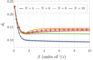
Figure 1: (Color online) Comparison of the results for the thermal expectation value (5) of the double occupancy $d_{i}$ stemming from exact diagonalization (solid lines) and TPQ states (circles) for a one-dimensional chain with periodic boundary conditions at $U_{i}=U=3J=3J_{ij}$. All TPQ results are calculated using a Krylov space dimension of $s=10$ except for the open circles in the $N=10$ case ($s=50$).

In Fig. 1 we exemplarily checked the convergence of TPQ results (circles) against results from exact diagonalization (solid lines) at half-filling and lattice sizes up to $N=10$. Even for comparably small Krylov dimensions $s=10$ a good agreement up to $N=8$, corresponding to $d=4900$ of the full Hilbert space, can be achieved. Only for $N=10$ sites ($d\approx$6.4\text{\times}{10}^{4}$$) the results of TPQ states start to deviate from the exact results. Using a Krylov space with $s=50$ is enough as a remedy leading again to a good convergence. This observation is in full accordance with the expectation that only small fractions of the overall Hilbert space are needed to yield accurate results in Krylov space procedures.

Before comparing KPM and TPQ to each other we point out that low temperatures $T$ result in large relative Boltzmann weights in Eqs. 17 and 18 for the low-energy part of the spectrum approximated by KPM. This, in turn, heavily amplifies even small numerical errors of stochastic or systematic origin. This spoils numerical results altogether for low temperatures. This issue is fundamental and cannot be solved by trivial means such as increasing the number of moments $\mu_{n}$. Approaches have been suggested to overcome these obstacles in the interacting regime by combining partial exact diagonalization and the kernel polynomial method Weiße et al. (2006). The ground state and the $m-1$ energetically lowest excitations of the systems are treated exactly while the remainder of the spectrum is calculated using KPM.

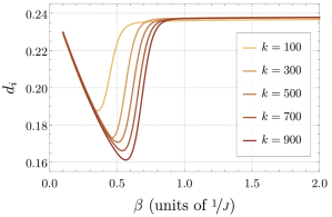
Figure 2: (Color online) Thermal expectation value of the double occupancy in a half-filled $N=10$ Hubbard chain at $U=3J$ calculated by KPM using $k$ moments $\mu_{n}$. The number of moments increases from top to bottom. A higher number of moments improves the accuracy, but it does not change the overall behavior for $\beta J>1$.

We illustrate the sketched caveat of KPM in its unmodified form described in Sec. III.2. Specifically, Fig. 2 displays KPM results which reproduce the physics at lower temperatures (larger inverse temperatures $\beta$) slightly better for a higher number $k$ of moments. But the true low-temperature limit, cf. Fig. 1, is not captured at all. The degree of double occupancy is significantly overestimated by KPM.

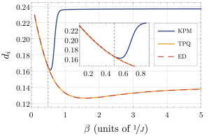
Figure 3: (Color online) Comparison of results from KPM ($k=900$) and TPQ states (Krylov space dimension $s=50$) with results from exact diagonalization (ED). KPM results show notable deviations for increasing $\beta$ while TPQ does not. Results for a half-filled Hubbard chain with periodic boundary conditions of $N=10$ sites at $U=3J$.

Nevertheless, we stress that the high-energy physics is captured very well by KPM. To emphasize this point the most accurate results of KPM for $k=900$ and the exact results (ED) are compared in the inset of Fig. 3. Although KPM results start deviating from the ED results at about $\beta\approx 0.5$ the high-energy physics for $T\gtrapprox 2J$ is described very accurately by KPM.

In contrast to KPM, using TPQ states is very robust against accumulating numerical errors since neither a functional approximation based on a truncated series nor a numerical integration is involved. In addition, TPQ states are easy to deal with. This makes this approach advantageous. Its convergence has been examined in detail Sugiura and Shimizu (2013) indicating that the choice of the individual random states $\ket{r}$ has an exponentially small effect at finite temperatures and that results from TPQ states converge to the actual ensemble results exponentially fast in the system size $N$. Thus, TPQ states can be used with predictable accuracy leading to well controlled results for a broad range of temperature as shown in Fig. 3. For this reason, all computations of thermal expectation values in the remainder of this article are performed using TPQ states. Two sources of errors need to be controlled: (i) the stochastic error in the evaluation of the traces and (ii) the systematic error in the evaluation of the matrix exponentials in Krylov spaces of finite dimension $s$.

IV Results

In this section, we tackle the issues of equilibration and thermalization on finite clusters. Temporal averages of expectation values and the corresponding temporal fluctuations will be discussed. The first section deals with equilibration, the subsequent one with thermalization.

IV.1 Equilibration

As outlined in the Introduction, analytic arguments for equilibration have been brought forward for the case of initial product states of system and bath Wilming et al. (2019). In order to extend evidence for equilibration beyond this special situation, we focus on the Fermi sea $\ket{\text{FS}}$ as generic non-product state in real space representation. The initial non-equilibrium is generated by an interaction quench according to (11).

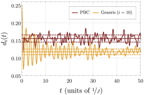
Figure 4: (Color online) Time evolution of the double occupancy on the integrable periodic Hubbard chain after interaction quench $U=3J$ and on the non-integrable (Generic) cluster of $N=12$ sites at half-filling. For the non-integrable case, the time evolution of cluster (l), see Appendix A, and its site $i=10$ is depicted and a one percent randomization around the average $U\approx 3J$ is chosen. Solid lines denote the average values (27), dashed lines the average plus and minus the standard deviation $\sigma_{i}$, both calculated at $\tau=$0.6$$.

In the highly excited state ensuing from the quench we examine the tendency of the finite clusters to equilibrate by simulating the time-dynamics of proper local observables which are measurable in the subsystem $S$. To study this phenomenon in detail we consider two types of clusters: (i) integrable ones with periodic boundary conditions (PBC) and a constant ratio $\nicefrac{{U}}{{J}}$ as well as (ii) generic clusters with an arbitrary topology. A complete overview over the used finite-size clusters is given in Appendix A. Henceforth, the labels (a), (b), … (n) ascribed to the individual topologies will be used for identifying a particular cluster. In order to avoid any undesired symmetries in the generic clusters, we additionally slightly randomize the parameters of the model such as the hopping strengths $J_{ij}=J_{ji}$ by drawing their values with uniform probability from the respective intervals $[J-p\cdot J;\,J+p\cdot J]$ with $p=0.01$. The same applies to the on-site interactions $U_{i}$ as well: they are taken from the interval $[U-p\cdot U;\,U+p\cdot U]$. Note that the randomization is deliberately chosen weak in order to avoid any many-body localization Nandkishore and Huse (2015). The only purpose of randomization is to avoid the influence of accidental symmetries. In the integrable clusters no randomization is performed because it would spoil the integrability.

As a meaningful local observable which incorporates two-particle interaction we choose the double occupancy $d_{i}=\widehat{n}_{{i\uparrow}}\widehat{n}_{{i\downarrow}}$. Thus, the subsystem $S$ consists of site $i$. For the calculation of the time-dependence we resort to CET as given in (15).

Results of the time-dependence in the integrable N=12 cluster and in the non-integrable cluster (l) of the same size are shown in Fig. 4 for half-filling and for $U=3J$. We clearly see signs of the expected fluctuations, see Introduction, around an average value without a tendency to converge to a constant stationary value. Even on longer time scales (not shown here) no constant stationary value is approached. This is to be attributed to the finite system size.

Interestingly, there seem to be indeed qualitative differences between the integrable and the generic cluster. The time series of the integrable cluster shows fluctuations which are of the same magnitude for all times. In contrast, the time series of the generic cluster first shows larger fluctuations which subsequently diminish to some extent. This observation, however, certainly needs to be substantiated further.

Next, we want to determine the long-time averages of the fluctuating quantities. These values are the best guesses on finite clusters for stationary values after relaxation. Since at the beginning there are various transient effects, see Fig. 4, it is not obvious how the long-time averages can be computed reliably. We account for this obstacle by introducing an averaging according to

$$\overline{d}(\tau):=\frac{1}{t_{\mathrm{max}}-t_{\mathrm{min}}}\int_{t_{\mathrm{min}}}^{t_{\mathrm{max}}}\differential{t}d(t)$$ (27)

with $\tau:=\nicefrac{{t_{\mathrm{min}}}}{{t_{\mathrm{max}}}}\in[0;1]$ for fixed values of $t_{\mathrm{max}}$. By tuning $\tau$ and thus the minimum time starting from which the averaging is performed we are able to eliminate the influence of initial relaxation effects on the dynamics. If not noted otherwise, all calculations are performed up to $t_{\mathrm{max}}=100/J$.

Exemplary results for all sites of the non-integrable, half-filled $N=12$ cluster (l), cf. Appendix A, are shown in Fig. 5. As can be seen, some weak initial transients are visible up to the range of $\tau\leq$0.2$$. During this initial time span we consider the data not fully converged yet, cf. especially the data for sites $i=6$ or $i=8$. After this initial transient, the averaged data converges to an almost constant value. But choosing $\tau$ too large, i.e., too close to unity, large fluctuations appear. The reason is that the averaged time span becomes too small so that the fluctuations do not cancel sufficiently anymore, cf. the range $\tau\gtrapprox$0.8$$ in Fig. 5. In conclusion, avoiding the initial transient effects as well as the final fluctuations can be achieved by reading off $\overline{d}_{i}$ for medium values, i.e., around $\tau\approx$0.5$$ to $\tau\approx$0.6$$.

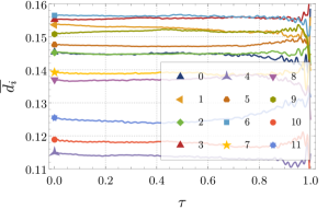
Figure 5: (Color online) Averages of the double occupancy of cluster (l) at the sites $i$ determined according to (27). A tendency of the dynamics to converge towards an essentially constant value around $\tau\approx$0.5$$ to $\tau\approx$0.6$$ is discernible for all sites.

In all checked cases of various lattice sizes $N$ and both integrable and non-integrable topology the determination of the time-averaged value according to (27) is possible since no significant variations occur in the range of $\tau\approx$0.5$$ to $\tau\approx$0.6$$. Thus, all following calculations are performed for a constant $\tau=$0.6$$. In this way, we obtain a suitable approximation of the stationary value of an observable $\overline{A}$ as discussed in Sec. I. We refer to these time-averages in the study of equilibration and thermalization.

For visual orientation, Fig. 4 shows the long-time averages (solid lines) and the standard deviations around them (dashed lines), both calculated at $\tau=0.6$. The initial dynamics differs qualitatively between the two cases considered. The generic model shows longer-lasting transients after the quench. Nevertheless, the long-time fluctuations show roughly the same amount of spread. This leads to the hypothesis that fluctuations show no pronounced dependence on the integrability of the model. We will substantiate this conjecture in the following.

The fluctuations present in the dynamics of the system around the time-averaged values $\overline{d}_{i}$ of the double occupancies are quantified by the individual variances $\sigma^{2}_{i}$. They are a measure for how well the (finite) system stays close to the time average $\overline{d}_{i}$. A fully equilibrating system would show vanishing fluctuations since it would fulfill $\lim_{t\to\infty}d_{i}(t)=\overline{d}_{i}$ so that $\sigma^{2}_{i}=0$ if the latter is determined for long, ideally infinite, time ranges. Practically, we use (27) also for the determination of the $\sigma^{2}_{i}$. We are not aware of analytic a priori predictions of the values of $\sigma^{2}_{i}$ in the physical situation we are considering, namely a highly entangled initial state in real space. Applying a scheme similar to (3) for an observable $O$ leads to an upper bound to its variance Short (2011) given by

$$\sigma_{O}^{2}\leq\frac{\Delta(O)^{2}}{4d_{\mathrm{eff}}(\omega)}\leq\frac{\norm{O}^{2}}{d_{\mathrm{eff}}(\omega)}$$ (28)

with $\norm{O}$ being the largest absolute eigenvalue of the Hermitian operator $O$ and

$$\Delta(O)=2\min_{c\in\mathbb{C}}\norm{O-c\mathbb{1}}.$$ (29)

Unfortunately, these upper bounds (28) still require the cumbersome calculation of the effective dimension as main ingredient which can neither be predicted without a complete diagonalization nor estimated except for initial product states of system and bath. For this reason, our main interest here is to study to which extent the considered systems equilibrate after their quench.

In order not to discuss each site in a cluster separately we define the global variance

$$\sigma^{2}=\frac{1}{N}\sum_{i=1}^{N}\sigma_{i}^{2}.$$ (30)

This quantity provides a good measure for the degree of equilibration. If it vanishes it indicates equilibration, at least on average. Fig. 6 depicts the global standard deviation $\sigma$. For the generic, non-integrable cluster the values for $\sigma^{2}$ are averaged additionally over all clusters of the same size $N$, see Appendix A, e.g., all generic clusters of $N=12$ sites are those labeled by (l)-(n). The plotted error bars indicate the average spread between the maximum and minimum standard deviation for each of the different clusters contributing to each data point for a specific cluster size $N$, i.e., half the error bar amounts to $\nicefrac{{1}}{{2}}(\sigma_{\mathrm{max}}-\sigma_{\mathrm{min}})$.

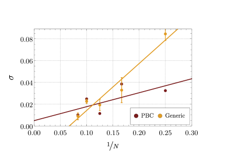
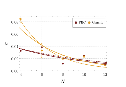
Figure 6: (Color online) Global standard deviations $\sigma$ as derived from (30) of the double occupancies $d_{i}(t)$ fluctuating around their individual average values $\overline{d}_{i}$. Results for both integrable (PBC) and non-integrable (Generic) clusters are shown. Three different least-square fits to the numerical data are displayed using either $\sigma=a_{0}+\nicefrac{{b_{0}}}{{N}}$ (upper panel), $\log(\sigma)=\log(a_{1})-b_{1}N$ (lower panel, solid lines) and $\sigma=a_{2}\exp(-b_{2}N)$ (lower panel, dashed lines). The latter two fits seem to be the same, but this is not the case because the condition of least squares depends on the functional form and leads to differing weights and thus to differing optimum sets $(a_{i},b_{i})$.

The first remarkable observation is that the standard deviations of the integrable and the non-integrable clusters are very similar for the same cluster size. One could have expected that the fluctuations in the integrable systems are larger because there is less accessible Hilbert space due to the large number of conserved quantities. But this does not seem to be the case. Furthermore, one could think that the similarity of the integrable and non-integrable fluctuations in Fig. 6 is at odds with the time series shown in Fig. 4 where the generic fluctuations are larger briefly after the quench. But for longer times this is no longer true and it is for these longer times that the quantity $\sigma$ is determined by definition, e.g., the evaluation at $\tau=0.6$ for $t_{\text{max}}=100/J$ implies that $\sigma$ is computed for the time interval $[60/J,100/J]$. In Fig. 4 the dashed lines and their mutual distance illustrate that the fluctuations of both systems are comparable in size.

In Fig. 6 we tackle the issue to extrapolate the data to the thermodynamic limit. To do so, we compare two kinds of fits with the first one being linear in the inverse lattice size, i.e., $\sigma=a+\nicefrac{{b}}{{N}}$ (upper panel) and the second one being exponential in the lattice size, i.e., $\sigma=a\exp\left(-bN\right)$ (lower panel). The exponential fit is carried out in two ways of least-square fits: (i) $\sigma$ is fitted with $a\exp\left(-bN\right)$, (ii) $\ln(\sigma)$ is fitted with $\ln(a)-bN$. The difference between both seemingly equal approaches lies in the least squares which are computed for $\sigma$ or $\ln(\sigma)$ implying different weights. The first procedure keeps the fit close to the data points at larger values of $\sigma$ while the second procedure focuses on the data points at smaller values.

We find that our data is consistent with the exponential scaling predicted Wilming et al. (2019). But the numerical data does not provide compelling evidence for the exponential scaling either. Thus, further study on this issue is certainly called for. However, both data sets and all fits regardless of the implied form of scaling indicate a vanishing global variance for $N\to\infty$. So this provides numerical evidence that equilibration takes place for systems of increasing system size. Equilibration appears to be the generic scenario independent of the property of integrability. This leads us to conclude that equilibration is an even more generic property than currently proven as it is neither limited by a highly entangled initial state nor by constants of motion present in integrable systems. These conclusions are corroborated by quenches to stronger interactions, for results see Appendix B for $U=6J$. For significantly weaker interaction quenches, the studied time scales and system sizes are not large enough to allow for unambiguous evidence, see Appendix B for $U=J$.

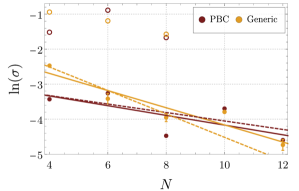
Figure 7: (Color online) Comparison of the actual global standard deviations $\sigma$ (filled symbols) to the upper bounds (open symbols) given by eq. 31 on logarithmic scale. The same fits and parameters as in the lower panel of Fig. 6 are shown; they appear here as straight lines.

For system sizes that are accessible to complete exact diagonalization we additionally determine the effective dimensions and the respective upper bounds (28) to variance and standard deviation. In this context, we compare the tightest upper bound for the double occupancies, i.e., $O=d_{i}$ and $c=\nicefrac{{1}}{{2}}$ in (29), leading to the upper bound

$$\sigma_{i}\leq\frac{1}{2}d_{\mathrm{eff}}(\omega)^{-\frac{1}{2}}.$$ (31)

The required effective dimension is computed assuming the absence of any degeneracy so that the following relation holds

$$\frac{1}{d_{\mathrm{eff}}(\omega)}=\sum_{n,j}\left(p_{j}\absolutevalue{\innerproduct{n}{\psi_{j}}}^{2}\right)^{2}.$$ (32)

Here, the initial state may be given as mixture $\rho(0)=\sum_{j}p_{j}\outerproduct{\psi_{j}}{\psi_{j}}$ and $\ket{n}$ denote the eigenstates of $H$.

The upper bounds are displayed by open symbols in the same color as the time-averaged standard deviations. The results and fits to the data are shown in Fig. 7 on a logarithmic scale. It is evident that the mathematically rigorous upper bounds are not particularly tight for the actually occurring fluctuations.

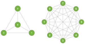
Figure 8: Infinite-range clusters for $N=4$ and $N=8$ denoting clusters with the maximum number of hoppings possible, also called complete graphs. For each of the $N$ sites the coordination number is $z=N-1$ leading to a total of $K=\nicefrac{{1}}{{2}}N(N-1)$ hopping links.

Discussing fluctuations it is interesting to consider the influence of the coordination number $z$. In the clusters considered so far, the typical coordination numbers is $z=2$ for the PBC and a mean value of $\overline{z}=$2.45$$ for the generic clusters. Hence these numbers do not vary much. But it is to be expected that systems with large coordination number display smaller fluctuations. At least in equilibrium, it is common lore that mean-field approaches work much better in higher dimensions and for larger coordination numbers because the relevance of the relative fluctuations is lower. Hence, the same presumption is a plausible working hypothesis out-of-equilibrium.

Here we want to test it for the accessible clusters. Due to the computational limitations in system size $N$ we choose to consider the limiting case of the maximum value of the coordination number. It is reached by linking each site with every other site implying $z=N-1$. The resulting clusters $G_{c}$ are called infinite-range clusters in physics and complete graphs in mathematics. In total, they have $K=\nicefrac{{1}}{{2}}N(N-1)$ bonds. The respective adjacency matrix reads

$$A(G_{c})=J_{N}-\mathbb{1}_{N}$$ (33)

where $J_{N}$ denotes the $N\times N$ all-ones-matrix and $\mathbb{1}_{N}$ stands for the identity matrix. We subtract the latter one to exclude local terms corresponding to hops from site $i$ to $i$. We point out that in infinite-range clusters without any randomization the initial Fermi sea state is highly degenerate leading to $\rho^{2}\ll\rho$. Due to this inherent self-averaging the fluctuations in fully symmetric clusters $G_{c}$ with the same $J$ on each bond and the same $U$ at each site are strongly suppressed (not shown). Since this is not what we want to study here we again slightly randomize the hoppings $J_{ij}$ and the interactions $U_{i}$ by $1\text{\,}\mathrm{\char 37\relax}$. This is exactly what we did for the generic clusters allowing for a study of the direct influence of large coordination numbers without being distracted by a large number of symmetries.

An example of two infinite-range graphs with $N=4$ and $N=8$, respectively, is given in Fig. 8. We use such clusters to compute the time-averaged double occupancies $\overline{d}_{i}$ and subsequently the global standard deviations $\sigma$ as before for (non-)integrable models in Fig. 6. No averaging over various clusters is conducted. The results are displayed in Fig. 9 and compared to the ones for integrable chains. Again, we insert the upper bounds for $\sigma_{i}$ determined by (31) by means of open symbols for small systems. A clear difference of the thermodynamic behavior, i.e., for $N\to\infty$, can be noticed. In PBC systems with a small coordination number the extrapolated fluctuations are noticeably larger than in the infinite-range clusters $G_{c}$. The standard deviations in the infinite-range clusters have a much steeper slope for increasing $N$ rendering fluctuations less important for larger complete graphs than for long PBC chains. This clearly supports the hypothesis that a larger connectivity favors smaller fluctuations. Hence, as a rule of thumb we expect that systems with larger coordination number equilibrate better than those with smaller coordination number. We stress that this finding does not necessarily imply that the equilibration occurs faster, i.e., on a shorter time scale. The issue of time scales is beyond the scope of the present article since the reliable determination of equilibration time scales is numerically very challenging.

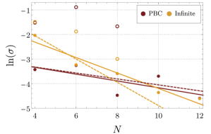
Figure 9: (Color online) Global standard deviations $\sigma$ of integrable chains with coordination number $z=2$ and of infinite-range clusters $G_{c}$ with $z=N-1$ and a one-percent randomization. Results are to be compared with Fig. 6. The amount of fluctuations depends on the number of bonds and decreases upon increasing coordination number so that the infinite-range clusters display only small fluctuations in the limit $N\to\infty$ relative to the fluctuations in the PBC clusters. The available upper bounds (31) are inserted using open symbols. Dashed and solid lines are fits, cf. Fig. 6.

IV.2 Thermalization

Here we address the process of thermalization. In the above Sec. IV.1 we noted no substantial influence of integrability on the degree of equilibration. In both cases of PBC and of the generic clusters the results indicated a stationary, equilibrated state in the thermodynamic limit. Moreover, the fluctuations due to the finite size of the studied clusters are comparable for the same system sizes.

In a next step, it suggests itself to investigate thermalization in the integrable chains and the generic clusters. To this end, we compare the equilibrated, time-averaged double occupancies $\overline{d}_{i}$ with the thermal predictions $\expectationvalue{d_{i}}_{\mathrm{th}}$ where the latter are computed for the canonical statistical ensemble at the same energy as the quenched system. Are they equal? In order not to be distracted by accidental effects at particular sites we define the global deviation from the thermalized values

$$\Delta_{\mathrm{therm}}:=\frac{1}{N}\sum_{i=1}^{N}\absolutevalue{\overline{d}_{i}-\expectationvalue{d_{i}}_{\mathrm{th}}}$$ (34)

for integrable (PBC) and non-integrable (generic) clusters of size $N$. The thermal predictions $\expectationvalue{d_{i}}_{\mathrm{th}}$ are calculated using TPQ states as described in Sec. III.3. Since each site $i$ of a given cluster contributes in (34) this definition accommodates for the highly differing individual topologies in a systematic way. A system showing perfect thermalization is characterized by a vanishing $\Delta_{\mathrm{therm}}=0$.

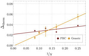
Figure 10: (Color online) Global deviation of the time-averages $\overline{d}_{i}$ from the thermal predictions $\expectationvalue{d_{i}}_{\mathrm{th}}$ at the effective temperature for $U=3J$. This deviation $\Delta_{\mathrm{therm}}$ is shown in dependence on the inverse cluster size $N$. For the generic clusters the shown values are averaged over various clusters of the same size and the error bar indicates the spread within this set of clusters. The lines represent linear regressions to the data.

Since we are dealing with closed quantum systems the total energy is conserved which allows us to determine the effective temperature of the system easily. Knowing the corresponding inverse temperature $\beta$ is necessary to compute the thermal expectation value of the cluster since it defines the statistical density matrix of the canonical ensemble. The initial state of the system, cf. Eq. 12 defines this effective temperature. It has an overall energy $E=\matrixelement{\mathrm{FS}}{H}{\mathrm{FS}}$ which translates into an effective inverse temperature according to Eq. 7.

In Fig. 10 the different global deviations are plotted against the inverse cluster sizes $N$ for the various topologies. Error bars again account for the spread of the values between the differently shaped clusters of same $N$ in the generic, non-integrable cases. In order to analyze the data, a linear fit $\Delta_{\mathrm{therm}}=\nicefrac{{A}}{{N}}+B$ is performed and included in the plot for both data sets. In accordance with previous studies Kinoshita et al. (2006); Rigol et al. (2007); Barthel and Schollwöck (2008); Kollar and Eckstein (2008); Eckstein and Kollar (2008); Rigol (2009); Tang et al. (2018) and with our expectations, clear trends can be read off. The generic, non-integrable clusters display a vanishing deviation $\Delta_{\mathrm{therm}}$ in the limit $N\to\infty$. This is a definite indication that theses clusters thermalize. In contrast, the integrable chains show only a slight decrease of the global deviation which is not consistent with a vanishing value for $N\to\infty$. The persisting finite value of $\Delta_{\mathrm{therm}}$ even for extrapolated infinitely large systems is a strong sign for equilibration of the integrable chains towards a non-thermal state. This must be attributed to the restricted dynamics due to the large number of constants of motion.

Since a perfectly thermalizing system loses all of its knowledge about the initial state $\rho(0)$ to the larger bath two borderline cases come to ones mind here. First, it is of interest whether a system which is only weakly perturbed, i.e., which is quenched to $\nicefrac{{U}}{{J}}\lessapprox 1$, is kept from thermalizing. Does a weak quench allow to retain memory about $\rho(0)$? Second, one can wonder whether quenches even stronger than $U=3J$ also lead to thermalization. We discuss both these questions in Appendix B for brevity.

V Summary

Using numerically exact methods we computed results for equilibration and thermalization of arbitrarily shaped finite-size clusters of the quenched Fermi-Hubbard model. The chosen initial state is the Fermi sea which is highly entangled in real space. The double occupancy is the local quantity of which the non-trivial quantum dynamics is studied after the interaction quenches.

We showed that even for the Fermi sea, which is a quantum state extremely far from a product state in real space, equilibration towards a stationary state is a generic property regardless of topology or integrability in the thermodynamic limit, i.e., for infinite system sizes. The fluctuations present in the finite systems are of comparable magnitude for various topologies and do not show a strong influence of integrability.

In addition, we studied infinite-range graphs which represent systems with maximum coordination number at given system size. It was found that the fluctuations in these graphs become significantly smaller for $N\to\infty$ than those in graphs of coordination number $z=2$. We stress that in infinite-range graphs the coordination number increases with system size $z=N-1$. This corroborates the expectation that fluctuations are less important for higher connectivity of the cluster. This paradigm is well established at equilibrium and the evidence found indicates that it holds true as well in non-equilibrium.

Concerning thermalization, we confirmed the expectations established in the literature that it depends decisively on the extent that integrals of motion exist. The integrable chains studied do not show thermalization, but stay away from the thermal canonical ensemble. In contrast, the generic clusters clearly display thermalization.

Obviously, many issues in the field of equilibration and thermalization still require intensive investigation. Our data showed that there are clear signs of transient behavior briefly after the quench before the long-time average values and variances emerge. For conceptual and practical purposes it is highly desirable to understand this transient behavior better, for instance by determining or at least estimating the relevant time scales. Knowledge of the relevant time scales in turn will help to compute long-time averages and stationary values with high accuracy. Finally, passing from quenches to more general forms of time-dependences of closed or open quantum systems represents a vast field of research.

Appendix A Finite clusters

Below, all clusters are presented which are used in the study of quenches in the generic non-integrable one-band Fermi-Hubbard model at half-filling. The $J_{ij}$ and $U_{i}$ have been chosen randomly in a uniform manner within a one-percent range around $J$ and $U$. The number of sites $N$ increases by two row by row starting from $N=4$ and going up to $N=12$.

(a)	(b)
(c)	(d)	(e)
(f)	(g)	(h)
(i)	(j)	(k)
(l)	(m)	(n)

Appendix B Additional results for $U=1J$ and $U=6J$

Additionally to the results for sudden interaction quenches to $U=3J$ provided in the main text, we simulated quenches to both $U=1J$ and $U=6J$. We again calculated the global standard deviation $\sigma$ as well as the global deviation $\Delta_{\mathrm{therm}}$. The respective results are thus comparable to the results shown in Fig. 6 and Fig. 10, respectively. Results for $U=1J$ are shown in Fig. 12 as well as in Fig. 12. The results for $U=6J$ are depicted in Fig. 14 as well as in Fig. 14.

Both for $U=1J$ and $U=6J$, we again notice a clear tendency of the global standard deviation $\sigma$ to decrease exponentially with increasing cluster size $N$, see Fig. 12 and Fig. 14. This is in full accordance with the results of quenches to $U=3J$ and corroborates our conclusion that this is the generic behavior.

The situation is slightly different for the thermalization behavior characterized by the global deviation $\Delta_{\mathrm{therm}}$ between actual results and thermal predictions. The predictions regarding thermalization with a vanishing $\Delta_{\mathrm{therm}}\to 0$ in the thermodynamic limit hold when the quenching strength is reasonably large, cf. Fig. 14. In situations, however, where the quench is comparably weak – which is the case when hopping strength $J$ and interaction $U$ are about equal at $U=1J$ – the system is only weakly perturbed. The amount of energy deposited in the system is relatively small. It is plausible that the effects induced by the lower amount of quenched energy make themselves felt only on larger time scales. Concomitantly, larger spatial scales are also required. While the computations can be done also for longer times with reasonable effort, increasing linearly in time, it is extremely tedious, if not impossible, to tackle larger systems because they have exponentially larger Hilbert spaces.

It is worthwhile to notice that the average spread of $\Delta_{\mathrm{therm}}$ among the generic clusters is much larger for $U=1J$ in Fig. 12 than in the other cases $U=3J$ and $U=6J$. This fact emphasizes the higher influence of the varying topology of the generic clusters for a particular system size $N$ for weak quenches. We attribute this to the fact that for weak interaction quenches the kinetic part of the Hamiltonian comprising the hoppings remains important. It is this part which defines the topology; for the local interaction any set of $N$ sites behaves the same.

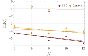
Figure 11: (Color online) Results for $U=1J$ showing the global standard deviation $\sigma$ as derived from (30) of the double occupancies $d_{i}(t)$ fluctuating around their average values $\overline{d}_{i}$ after interaction quenches. In accordance with Fig. 6 fluctuations are becoming exponentially smaller with increasing cluster size $N$. Upper bounds (31) are computed by complete exact diagonalization and shown using open symbols. The bounds are indeed well above the actual data, but they are clearly not tight. Solid and dashed lines denote fits, cf. Fig. 6.

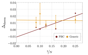
Figure 12: (Color online) Results for an interaction quench of the strength $U=1J$ showing the global deviation $\Delta_{\mathrm{therm}}$ of the time-averages $\overline{d}_{i}$ from the thermal predictions $\expectationvalue{d_{i}}_{\mathrm{th}}$ at the effective temperature of the quench. Integrable (PBC) and non-integrable (Generic) clusters are shown. A pronounced spread between the different generic clusters can be noticed. Since the system is only weakly quenched no clear tendency of thermalization or the absence thereof is visible in the data for both the PBC and the generic systems.

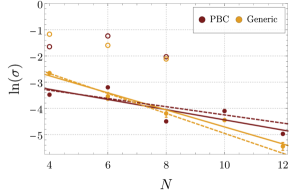
Figure 13: (Color online) Global standard deviations $\sigma$ for $U=6J$ as derived from (30). The tendency of the fluctuations to decrease exponentially with increasing system size $N$ is obvious. Open symbols show upper bounds (31).

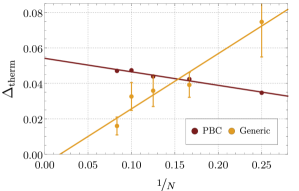
Figure 14: (Color online) Global deviation of the time-averages $\overline{d}_{i}$ from the thermal predictions $\expectationvalue{d_{i}}_{\mathrm{th}}$ at the effective temperature for $U=6J$. The results agree qualitatively with the ones shown in Fig. 10 where a detailed analysis can be found.