Quantifying Attention Flow in Transformers

Abstract

In the Transformer model, “self-attention” combines information from attended embeddings into the representation of the focal embedding in the next layer. Thus, across layers of the Transformer, information originating from different tokens gets increasingly mixed. This makes attention weights unreliable as explanations probes. In this paper, we consider the problem of quantifying this flow of information through self-attention. We propose two methods for approximating the attention to input tokens given attention weights, attention rollout and attention flow, as post hoc methods when we use attention weights as the relative relevance of the input tokens. We show that these methods give complementary views on the flow of information, and compared to raw attention, both yield higher correlations with importance scores of input tokens obtained using an ablation method and input gradients.

1 Introduction

Attention (Bahdanau et al., 2015; Vaswani et al., 2017) has become the key building block of neural sequence processing models, and visualizing attention weights is the easiest and most popular approach to interpret a model’s decisions and to gain insights about its internals (Vaswani et al., 2017; Xu et al., 2015; Wang et al., 2016; Lee et al., 2017; Dehghani et al., 2019; Rocktäschel et al., 2016; Chen and Ji, 2019; Coenen et al., 2019; Clark et al., 2019). Although it is wrong to equate attention with explanation  (Pruthi et al., 2019; Jain and Wallace, 2019), it can offer plausible and meaningful interpretations (Wiegreffe and Pinter, 2019; Vashishth et al., 2019; Vig, 2019). In this paper, we focus on problems arising when we move to the higher layers of a model, due to lack of token identifiability of the embeddings in higher layers (Brunner et al., 2020).

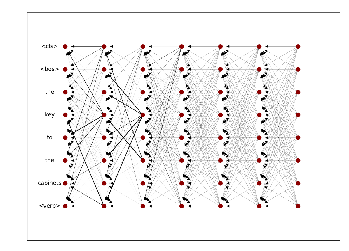
(a) Embedding attentions

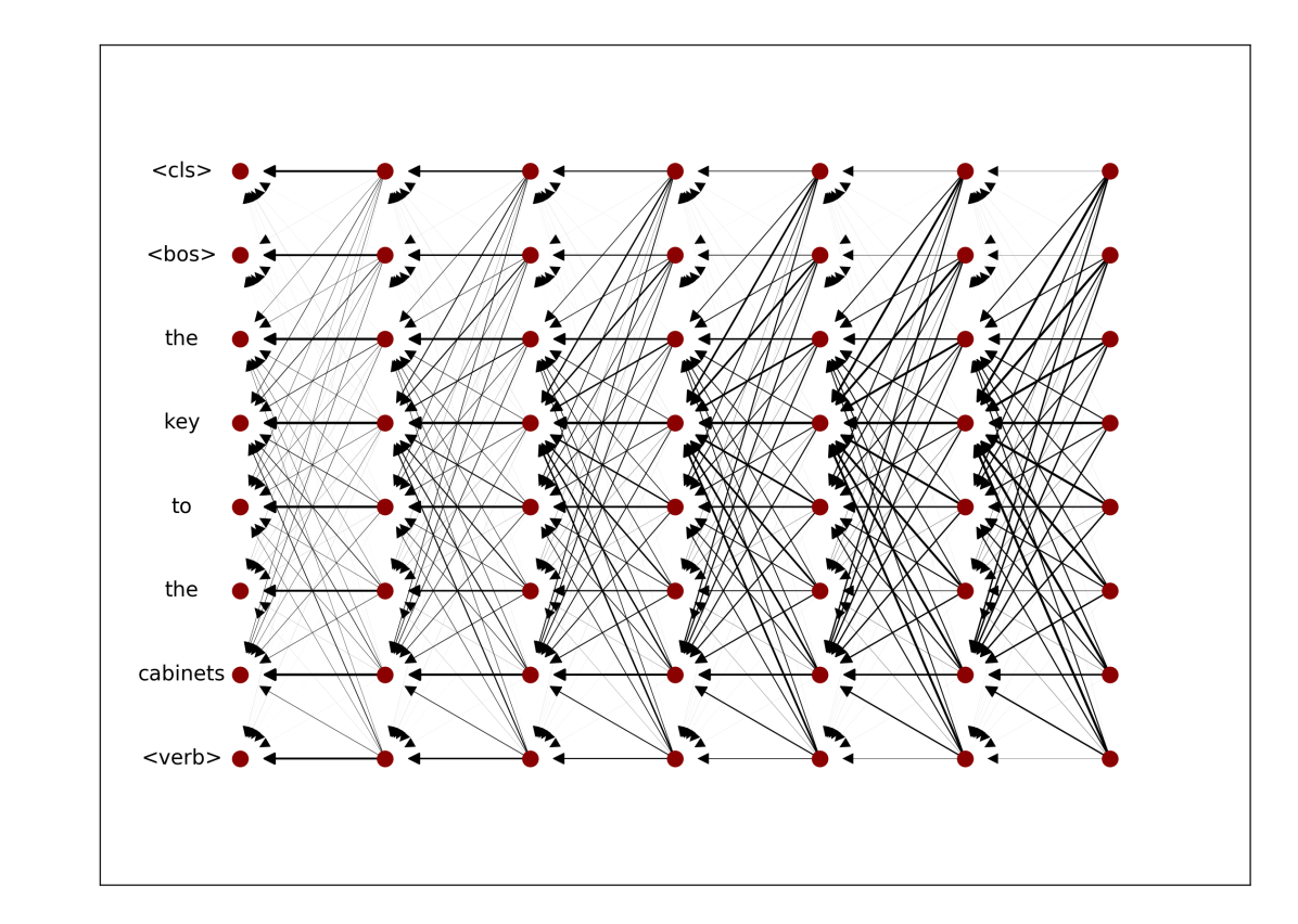
(b) Attention rollout

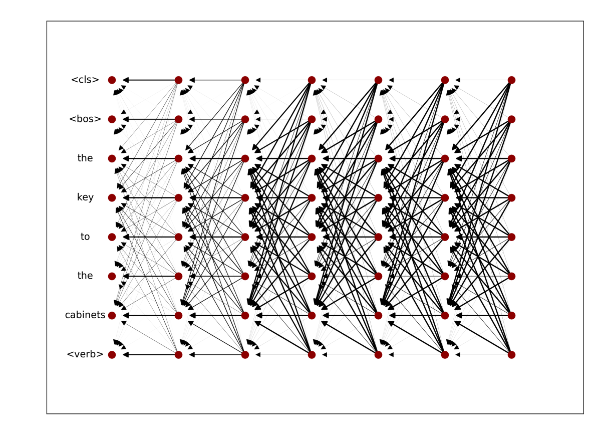
(c) Attention flow

Figure 1: Visualisation of attention weights.

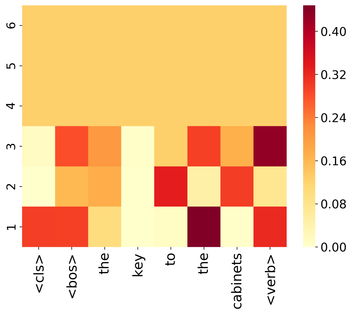
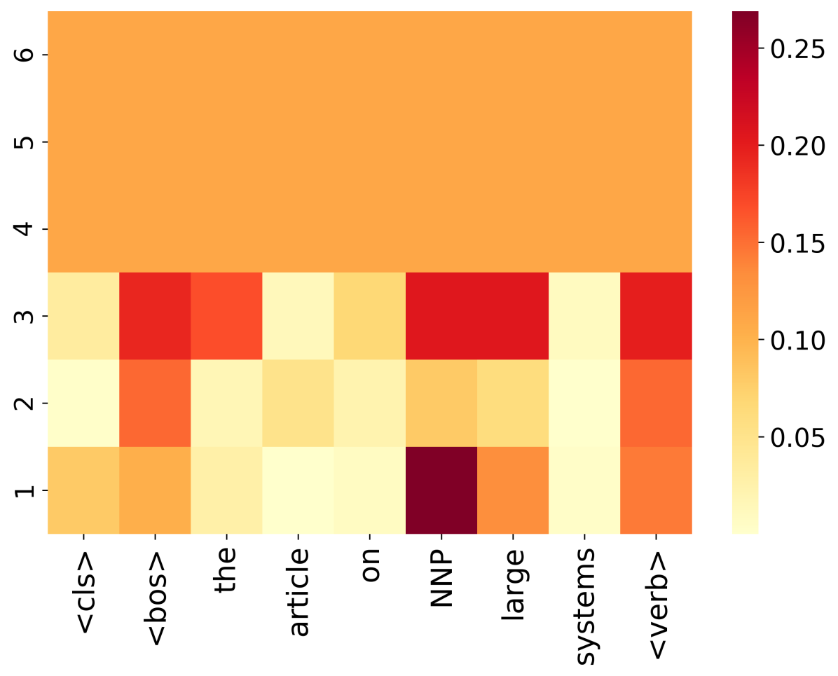
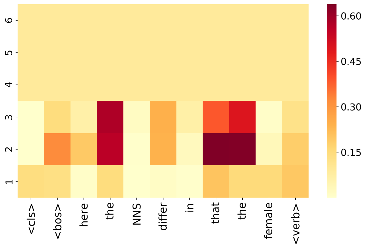
Figure 2: Raw Attention maps for the CLS token at different layers.

We propose two simple but effective methods to compute attention scores to input tokens (i.e., token attention) at each layer, by taking raw attentions (i.e., embedding attention) of that layer as well as those from the precedent layers. These methods are based on modelling the information flow in the network with a DAG (Directed Acyclic Graph), in which the nodes are input tokens and hidden embeddings, edges are the attentions from the nodes in each layer to those in the previous layer, and the weights of the edges are the attention weights. The first method, attention rollout, assumes that the identities of input tokens are linearly combined through the layers based on the attention weights. To adjust attention weights, it rolls out the weights to capture the propagation of information from input tokens to intermediate hidden embeddings. The second method, attention flow, considers the attention graph as a flow network. Using a maximum flow algorithm, it computes maximum flow values, from hidden embeddings (sources) to input tokens (sinks). In both methods, we take the residual connection in the network into account to better model the connections between input tokens and hidden embedding. We show that compared to raw attention, the token attentions from attention rollout and attention flow have higher correlations with the importance scores obtained from input gradients as well as blank-out, an input ablation based attribution method. Furthermore, we visualize the token attention weights and demonstrate that they are better approximations of how input tokens contribute to a predicted output, compared to raw attention.

It is noteworthy that the techniques we propose in this paper, are not toward making hidden embeddings more identifiable, or providing better attention weights for better performance, but a new set of attention weights that take token identity problem into consideration and can serve as a better diagnostic tool for visualization and debugging.

2 Setups and Problem Statement

In our analysis, we focus on the verb number prediction task, i.e., predicting singularity or plurality of a verb of a sentence, when the input is the sentence up to the verb position. We use the subject-verb agreement dataset (Linzen et al., 2016). This task and dataset are convenient choices, as they offer a clear hypothesis about what part of the input is essential to get the right solution. For instance, given “the key to the cabinets” as the input, we know that attending to “key” helps the model predict singular as output while attending to “cabinets” (an agreement attractor, with the opposite number) is unhelpful.

We train a Transformer encoder, with GPT-2 Transformer blocks as described in (Radford et al., 2019; Wolf et al., 2019) (without masking). The model has 6 layers, and 8 heads, with hidden/embedding size of 128. Similar to Bert (Devlin et al., 2019) we add a CLS token and use its embedding in the final layer as the input to the classifier. The accuracy of the model on the subject-verb agreement task is $0.96$. To facilitate replication of our experiments we will make the implementations of the models we use and algorithms we introduce publicly available at https://github.com/samiraabnar/attention_flow.

We start by visualizing raw attention in Figure 1(a) (like Vig 2019). The example given here is correctly classified. Crucially, only in the first couple of layers, there are some distinctions in the attention patterns for different positions, while in higher layers the attention weights are rather uniform. Figure 2 (left) gives raw attention scores of the CLS token over input tokens (x-axis) at different layers (y-axis), which similarly lack an interpretable pattern.These observations reflect the fact that as we go deeper into the model, the embeddings are more contextualized and may all carry similar information. This underscores the need to track down attention weights all the way back to the input layer and is in line with findings of Serrano and Smith (2019), who show that attention weights do not necessarily correspond to the relative importance of input tokens.

To quantify the usefulness of raw attention weights, and the two alternatives that we consider in the next section, besides input gradients, we employ an input ablation method, blank-out, to estimate an importance score for each input token. Blank-out replaces each token in the input, one by one, with UNK and measures how much it affects the predicted probability of the correct class. We compute the Spearman’s rank correlation coefficient between the attention weights of the CLS embedding in the final layer and the importance scores from blank-out. As shown in the first row of Table 1, the correlation between raw attention weights of the CLS token and blank-out scores is rather low, except for the first layer. As we can see in Table 2 this is also the case when we compute the correlations with input gradients.

	L1	L2	L3	L4	L5	L6
Raw	0.69$\pm$0.27	0.10$\pm$0.43	-0.11$\pm$0.49	-0.09$\pm$0.52	0.20$\pm$0.45	0.29$\pm$0.39
Rollout	0.32$\pm$0.26	0.38$\pm$0.27	0.51$\pm$0.26	0.62$\pm$0.26	0.70$\pm$0.25	0.71$\pm$0.24
Flow	0.32$\pm$0.26	0.44$\pm$0.29	0.70$\pm$0.25	0.70$\pm$0.22	0.71$\pm$0.22	0.70$\pm$0.22

Table 1: SpearmanR correlation of attention based importance with blank-out scores for 2000 samples from the test set for the verb number prediction model.

	L1	L2	L3	L4	L5	L6
Raw	0.53$\pm$0.33	0.16$\pm$0.38	-0.06$\pm$0.42	0.00$\pm$0.47	0.24$\pm$0.40	0.46$\pm$0.35
Rollout	0.22$\pm$0.31	0.27$\pm$0.32	0.39$\pm$0.32	0.47$\pm$0.32	0.53$\pm$0.32	0.54$\pm$0.31
Flow	0.22$\pm$0.31	0.31$\pm$0.34	0.54$\pm$0.32	0.61$\pm$0.28	0.60$\pm$0.28	0.61$\pm$0.28

Table 2: SpearmanR correlation of attention based importance with input gradients for 2000 samples from the test set for the verb number prediction model.

3 Attention Rollout and Attention Flow

Attention rollout and attention flow recursively compute the token attentions in each layer of a given model given the embedding attentions as input. They differ in the assumptions they make about how attention weights in lower layers affect the flow of information to the higher layers and whether to compute the token attentions relative to each other or independently.

To compute how information propagates from the input layer to the embeddings in higher layers, it is crucial to take the residual connections in the model into account as well as the attention weights. In a Transformer block, both self-attention and feed-forward networks are wrapped by residual connections, i.e., the input to these modules is added to their output. When we only use attention weights to approximate the flow of information in Transformers, we ignore the residual connections. But these connections play a significant role in tying corresponding positions in different layers. Hence, to compute attention rollout and attention flow, we augment the attention graph with extra weights to represent residual connections. Given the attention module with residual connection, we compute values in layer $l+1$ as $V_{l+1}=V_{l}+W_{att}V_{l}$, where $W_{att}$ is the attention matrix. Thus, we have $V_{l+1}=(W_{att}+I)V_{l}$. So, to account for residual connections, we add an identity matrix to the attention matrix and re-normalize the weights. This results in $A=0.5W_{att}+0.5I$, where $A$ is the raw attention updated by residual connections.

Furthermore, analyzing individual heads requires accounting for mixing of information between heads through a position-wise feed-forward network in Transformer block. Using attention rollout and attention flow, it is also possible to analyze each head separately. We explain in more details in Appendix A.1. However, in our analysis in this paper, for simplicity, we average the attention at each layer over all heads.

Attention rollout

Attention rollout is an intuitive way of tracking down the information propagated from the input layer to the embeddings in the higher layers. Given a Transformer with $L$ layers, we want to compute the attention from all positions in layer $l_{i}$ to all positions in layer $l_{j}$, where $j<i$. In the attention graph, a path from node $v$ at position $k$ in $l_{i}$, to node $u$ at position $m$ in $l_{j}$, is a series of edges that connect these two nodes. If we look at the weight of each edge as the proportion of information transferred between two nodes, we can compute how much of the information at $v$ is propagated to $u$ through a particular path by multiplying the weights of all edges in that path. Since there may be more than one path between two nodes in the attention graph, to compute the total amount of information propagated from $v$ to $u$, we sum over all possible paths between these two nodes. At the implementation level, to compute the attentions from $l_{i}$ to $l_{j}$, we recursively multiply the attention weights matrices in all the layers below.

$$\tilde{A}(l_{i})=\left\{\begin{array}[]{@{}ll@{}}A(l_{i})\tilde{A}(l_{i-1})&\mbox{if}~{}i>j\\ A(l_{i})&\mbox{if}~{}i=j\end{array}\right.$$ (1)

In this equation, $\tilde{A}$ is attention rollout, $A$ is raw attention and the multiplication operation is a matrix multiplication. With this formulation, to compute input attention we set $j=0$.

Attention flow

In graph theory, a flow network is a directed graph with a “capacity” associated with each edge. Formally, given $G=(V,E)$ is a graph, where $V$ is the set of nodes, and $E$ is the set of edges in $G$; $C=\{c_{uv}\in\mathbb{R}~{}|~{}\forall{u,v}~{}\mathrm{where}~{}e_{u,v}\in E\land u\neq v\}$ denotes the capacities of the edges and $s,t\in V$ are the source and target (sink) nodes respectively; flow is a mapping of edges to real numbers, $f:E\to\mathbb{R}$, that satisfies two conditions: (a) capacity constraint: for each edge the flow value should not exceed its capacity, $|f_{uv}\leq c_{uv}|$; (b) flow conservation: for all nodes except $s$ and $t$ the input flow should be equal to output flow –sum of the flow of outgoing edges should be equal to sum of the flow of incoming edges. Given a flow network, a maximum flow algorithm finds a flow which has the maximum possible value between $s$ and $t$ (Cormen et al., 2009).

Treating the attention graph as a flow network, where the capacities of the edges are attention weights, using any maximum flow algorithm, we can compute the maximum attention flow from any node in any of the layers to any of the input nodes. We can use this maximum-flow-value as an approximation of the attention to input nodes. In attention flow, the weight of a single path is the minimum value of the weights of the edges in the path, instead of the product of the weights. Besides, we can not compute the attention for node $s$ to node $t$ by adding up the weights of all paths between these two nodes, since there might be an overlap between the paths and this might result in overflow in the overlapping edges.

It is noteworthy that both of the proposed methods can be computed in polynomial time. $O(d*n^{2})$ for attention rollout and $O(d^{2}*n^{4})$ for attention flow, where $d$ is the depth of the model, and $n$ is the number of tokens.

Figure 3: Attention maps for the CLS token

.

4 Analysis and Discussion

Now, we take a closer look at these three views of attention. Figure 1 depicts raw attention, attention rollout and attention flow for a correctly classified example across different layers. It is noteworthy that the first layer of attention rollout and attention flow are the same, and their only difference with raw attention is the addition of residual connections. As we move to the higher layers, we see that the residual connections fade away. Moreover, in contrast to raw attention, the patterns of attention rollout and attention flow become more distinctive in the higher layers.

Figures 2 and 3 show the weights from raw attention, attention rollout and attention flow for the CLS embedding over input tokens (x-axis) in all 6 layers (y-axis) for three examples. The first example is the same as the one in Figure 1. The second example is “the article on NNP large systems <?>”. The model correctly classifies this example and changing the subject of the missing verb from “article” to “articles” flips the decision of the model. The third example is “here the NNS differ in that the female <?>”, which is a miss-classified example and again changing “NNS” (plural noun) to “NNP” (singular proper noun) flips the decision of the model.

For all cases, the raw attention weights are almost uniform above layer three (discussed before). In the case of the correctly classified example, we observe that both attention rollout and attention flow assign relatively high weights to both the subject of the verb, “article’ and the attractor, “systems”. For the miss-classified example, both attention rollout and attention flow assign relatively high scores to the “NNS” token which is not the subject of the verb. This can explain the wrong prediction of the model.

The main difference between attention rollout and attention flow is that attention flow weights are amortized among the set of most attended tokens, as expected. Attention flow can indicate a set of input tokens that are important for the final decision. Thus we do not get sharp distinctions among them. On the other hand, attention rollout weights are more focused compared to attention flow weights, which is sensible for the third example but not as much for the second one.

	L1	L3	L5	L6
Raw	0.12 $\pm$ 0.21	0.09 $\pm$ 0.21	0.08 $\pm$ 0.20	0.09 $\pm$ 0.21
Rollout	0.11 $\pm$ 0.19	0.12 $\pm$ 0.21	0.13 $\pm$ 0.21	0.13 $\pm$ 0.20
Flow	0.11 $\pm$ 0.19	0.11 $\pm$ 0.21	0.12 $\pm$ 0.22	0.14 $\pm$ 0.21

Table 3: SpearmanR correlation of attention based importance with input gradients for 100 samples from the test set for the DistillBERT model fine tuned on SST-2.

(a) “The author talked to Sara about mask book.”

(b) “Mary convinced John of mask love.”

Figure 4: Bert attention maps. We look at the attention weights from the mask embedding to the two potential references for it, e.g. “author” and “Sara” in (a) and “Mary” and “John” in (b). The bars, at the left, show the relative predicted probability for the two possible pronouns, “his” and “her”.

Furthermore, as shown in Table 1 and 2 both attention rollout and attention flow, are better correlated with blank-out scores and input gradients compared to raw attention, but attention flow weights are more reliable than attention rollout. The difference between these two methods is rooted in their different views of attention weights. Attention flow views them as capacities, and at every step of the algorithm, it uses as much of the capacity as possible. Hence, attention flow computes the maximum possibility of token identities to propagate to the higher layers. Whereas attention rollout views them as proportion factors and at every step, it allows token identities to be propagated to higher layers exactly based on this proportion factors. This makes attention rollout stricter than attention flow, and so we see that attention rollout provides us with more focused attention patterns. However, since we are making many simplifying assumptions, the strictness of attention rollout does not lead to more accurate results, and the relaxation of attention flow seems to be a useful property.

At last, to illustrate the application of attention flow and attention rollout on different tasks and different models, we examine them on two pretrained BERT models. We use the models available at https://github.com/huggingface/transformers.

Table 3 shows the correlation of the importance score obtained from raw attention, attention rollout and attention flow from a DistillBERT (Sanh et al., 2019) model fine-tuned to solve “SST-2” (Socher et al., 2013), the sentiment analysis task from the glue benchmark (Wang et al., 2018). Even though for this model, all three methods have very low correlation with the input gradients, we can still see that attention rollout and attention flow are slightly better than raw attention.

Furthermore, in Figure 4, we show an example of applying these methods to a pre-trained Bert to see how it resolves the pronouns in a sentence. What we do here is to feed the model with a sentence, masking a pronoun. Next, we look at the prediction of the model for the masked word and compare the probabilities assigned to “her” and “his”. Then we look at raw attention, attention rollout and attention flow weights of the embeddings for the masked pronoun at all the layers. In the first example, in Figure 4(a), attention rollout and attention flow are consistent with each other and the prediction of the model. Whereas, the final layer of raw attention does not seem to be consistent with the prediction of the models, and it varies a lot across different layers. In the second example, in Figure 4(b), only attention flow weights are consistent with the prediction of the model.

5 Conclusion

Translating embedding attentions to token attentions can provide us with better explanations about models’ internals. Yet, we should be cautious about our interpretation of these weights, because, we are making many simplifying assumptions when we approximate information flow in a model with the attention weights. Our ideas are simple and task/architecture agnostic. In this paper, we insisted on sticking with simple ideas that only require attention weights and can be easily employed in any task or architecture that uses self-attention. We should note that all our analysis in this paper is for a Transformer encoder, with no casual masking. Since in Transformer decoder, future tokens are masked, naturally there is more attention toward initial tokens in the input sequence, and both attention rollout and attention flow will be biased toward these tokens. Hence, to apply these methods on a Transformer decoder, we should first normalize based on the receptive field of attention.

Following this work, we can build the attention graph with effective attention weights (Brunner et al., 2020) instead of raw attentions. Furthermore, we can come up with a new method that adjusts the attention weights using gradient-based attribution methods (Ancona et al., 2019).

Appendix A Appendices

A.1 Single Head Analysis

For analysing the attention weights, with multi-head setup, we could either analyze attention heads separately, or we could average all heads and have a single attention graph. However, we should be careful that treating attention heads separately could potentially mean that we are assuming there is no mixing of information between heads, which is not true as we combine information of heads in the position-wise feed-forward network on top of self-attention in a transformer block. It is possible to analyse the role of each head in isolation of all other heads using attention rollout and attention flow. To not make the assumption that there is no mixing of information between heads, for computing the “input attention”, we will treat all the layers below the layer of interest as single head layers, i.e., we sum the attentions of all heads in the layers below. For example, we can compute attention rollout for head $k$ at layer $i$ as $\tilde{A}(i,k)=A(i,k)\bar{A}_{(}i)$, where, $\bar{A}_{(}i)$ is attention rollout computed for layer $i$ with the single head assumption.

References

- Ancona et al. (2019) Marco Ancona, Enea Ceolini, Cengiz Öztireli, and Markus Gross. 2019. Gradient-Based Attribution Methods, pages 169–191. Springer International Publishing.
- Bahdanau et al. (2015) Dzmitry Bahdanau, Kyunghyun Cho, and Yoshua Bengio. 2015. Neural machine translation by jointly learning to align and translate. In proceedings of the 2015 International Conference on Learning Representations.
- Brunner et al. (2020) Gino Brunner, Yang Liu, Damian Pascual, Oliver Richter, Massimiliano Ciaramita, and Roger Wattenhofer. 2020. On identifiability in transformers. In International Conference on Learning Representations.
- Chen and Ji (2019) Hanjie Chen and Yangfeng Ji. 2019. Improving the interpretability of neural sentiment classifiers via data augmentation. arXiv preprint arXiv:1909.04225.
- Clark et al. (2019) Kevin Clark, Urvashi Khandelwal, Omer Levy, and Christopher D. Manning. 2019. What does BERT look at? an analysis of BERT’s attention. In Proceedings of the 2019 ACL Workshop BlackboxNLP: Analyzing and Interpreting Neural Networks for NLP, pages 276–286, Florence, Italy. Association for Computational Linguistics.
- Coenen et al. (2019) Andy Coenen, Emily Reif, Ann Yuan, Been Kim, Adam Pearce, Fernanda Viégas, and Martin Wattenberg. 2019. Visualizing and measuring the geometry of bert. arXiv preprint arXiv:1906.02715.
- Cormen et al. (2009) Thomas H. Cormen, Charles E. Leiserson, Ronald L. Rivest, and Clifford Stein. 2009. Introduction to Algorithms, Third Edition, 3rd edition. The MIT Press.
- Dehghani et al. (2019) Mostafa Dehghani, Stephan Gouws, Oriol Vinyals, Jakob Uszkoreit, and Łukasz Kaiser. 2019. Universal transformers. In proceedings of the 2019 International Conference on Learning Representations.
- Devlin et al. (2019) Jacob Devlin, Ming-Wei Chang, Kenton Lee, and Kristina Toutanova. 2019. BERT: Pre-training of deep bidirectional transformers for language understanding. In proceedings of the 2019 Conference of the North American Chapter of the Association for Computational Linguistics: Human Language Technologies. Association for Computational Linguistics.
- Jain and Wallace (2019) Sarthak Jain and Byron C. Wallace. 2019. Attention is not Explanation. In proceedings of the 2019 Conference of the North American Chapter of the Association for Computational Linguistics: Human Language Technologies, pages 3543–3556. Association for Computational Linguistics.
- Lee et al. (2017) Jaesong Lee, Joong-Hwi Shin, and Jun-Seok Kim. 2017. Interactive visualization and manipulation of attention-based neural machine translation. In proceedings of the 2017 Conference on Empirical Methods in Natural Language Processing: System Demonstrations, pages 121–126.
- Linzen et al. (2016) Tal Linzen, Emmanuel Dupoux, and Yoav Goldberg. 2016. Assessing the ability of LSTMs to learn syntax-sensitive dependencies. Transactions of the Association for Computational Linguistics, 4:521–535.
- Pruthi et al. (2019) Danish Pruthi, Mansi Gupta, Bhuwan Dhingra, Graham Neubig, and Zachary C Lipton. 2019. Learning to deceive with attention-based explanations. arXiv preprint arXiv:1909.07913.
- Radford et al. (2019) Alec Radford, Jeffrey Wu, Rewon Child, David Luan, Dario Amodei, and Ilya Sutskever. 2019. Language models are unsupervised multitask learners. OpenAI Blog, 1(8).
- Rocktäschel et al. (2016) Tim Rocktäschel, Edward Grefenstette, Karl Moritz Hermann, Tomas Kocisky, and Phil Blunsom. 2016. Reasoning about entailment with neural attention. In International Conference on Learning Representations (ICLR).
- Sanh et al. (2019) Victor Sanh, Lysandre Debut, Julien Chaumond, and Thomas Wolf. 2019. Distilbert, a distilled version of bert: smaller, faster, cheaper and lighter.
- Serrano and Smith (2019) Sofia Serrano and Noah A. Smith. 2019. Is attention interpretable? In proceedings of the 57th Annual Meeting of the Association for Computational Linguistics. Association for Computational Linguistics.
- Socher et al. (2013) Richard Socher, Alex Perelygin, Jean Wu, Jason Chuang, Christopher D. Manning, Andrew Ng, and Christopher Potts. 2013. Recursive deep models for semantic compositionality over a sentiment treebank. In Proceedings of the 2013 Conference on Empirical Methods in Natural Language Processing, pages 1631–1642, Seattle, Washington, USA. Association for Computational Linguistics.
- Vashishth et al. (2019) Shikhar Vashishth, Shyam Upadhyay, Gaurav Singh Tomar, and Manaal Faruqui. 2019. Attention interpretability across nlp tasks. arXiv preprint arXiv:1909.11218.
- Vaswani et al. (2017) Ashish Vaswani, Noam Shazeer, Niki Parmar, Jakob Uszkoreit, Llion Jones, Aidan N Gomez, Łukasz Kaiser, and Illia Polosukhin. 2017. Attention is all you need. In Advances in neural information processing systems, pages 5998–6008.
- Vig (2019) Jesse Vig. 2019. Visualizing attention in transformer-based language models. arXiv preprint arXiv:1904.02679.
- Wang et al. (2018) Alex Wang, Amanpreet Singh, Julian Michael, Felix Hill, Omer Levy, and Samuel Bowman. 2018. GLUE: A multi-task benchmark and analysis platform for natural language understanding. In Proceedings of the 2018 EMNLP Workshop BlackboxNLP: Analyzing and Interpreting Neural Networks for NLP, pages 353–355, Brussels, Belgium. Association for Computational Linguistics.
- Wang et al. (2016) Yequan Wang, Minlie Huang, Li Zhao, et al. 2016. Attention-based lstm for aspect-level sentiment classification. In proceedings of the 2016 conference on empirical methods in natural language processing, pages 606–615.
- Wiegreffe and Pinter (2019) Sarah Wiegreffe and Yuval Pinter. 2019. Attention is not not explanation. In proceedings of the 2019 Conference on Empirical Methods in Natural Language Processing and the 9th International Joint Conference on Natural Language Processing (EMNLP-IJCNLP). Association for Computational Linguistics.
- Wolf et al. (2019) Thomas Wolf, Lysandre Debut, Victor Sanh, Julien Chaumond, Clement Delangue, Anthony Moi, Pierric Cistac, Tim Rault, R’emi Louf, Morgan Funtowicz, and Jamie Brew. 2019. Huggingface’s transformers: State-of-the-art natural language processing. ArXiv, abs/1910.03771.
- Xu et al. (2015) Kelvin Xu, Jimmy Ba, Ryan Kiros, Kyunghyun Cho, Aaron Courville, Ruslan Salakhudinov, Rich Zemel, and Yoshua Bengio. 2015. Show, attend and tell: Neural image caption generation with visual attention. In proceedings of International Conference on Machine Learning, pages 2048–2057.