Pattern-Based Analysis of Time Series: Estimation

Abstract

While Internet of Things (IoT) devices and sensors create continuous streams of information, Big Data infrastructures are deemed to handle the influx of data in real-time. One type of such a continuous stream of information is time series data. Due to the richness of information in time series and inadequacy of summary statistics to encapsulate structures and patterns in such data, development of new approaches to learn time series is of interest. In this paper, we propose a novel method, called pattern tree, to learn patterns in the times-series using a binary-structured tree. While a pattern tree can be used for many purposes such as lossless compression, prediction and anomaly detection, in this paper we focus on its application in time series estimation and forecasting. In comparison to other methods, our proposed pattern tree method improves the mean squared error of estimation.

I Introduction

With the enormous amount of data being collected by the smart devices and sensors, Internet of Things (IoT), high resolution time series are becoming one of the main types of Big Data. Due to the long temporal length and high temporal resolution of time series, efficient processing of such data can be challenging. One possibility is characterization through low order statistics, but such approaches may lead to the loss of information-rich parts of time series, since in many applications most of the value in the information is in the parts that deviates from the low order statistics, i.e. in the atypical parts [1, 2]. For example, consider the heart rate time series recorded by wearables that are being used as remote health monitoring devices (IoT in health care [3]), there are short-duration arrhythmic patterns that are valuable in the sense that they are known to indicate possible onset of disease, but not fully reflected in simple summary statistics like the sample mean, variance or covariance. Another example is stock market data, for which hourly stock data is more eventful than the daily data. Hence, the availability of such time series data and the richness of information they contain encourage new approaches in order to efficiently learn the structure of the time series, and extract patterns for more accurate processing (e.g. estimation, prediction and detection).

Regression and classification trees (CART) and random forests [4] constitute a general approach to non-parametric analysis of data developed in the early 1980’s. More recently, model-free pattern-based analysis has been considered in the literature [5, 6, 7, 8, 9, 10, 11, 12, 13]. Kozat et al. [14] used a universal prediction approach, called a context tree to partition the regressors space resulting in a piece-wise linear prediction technique. Chung et al. [5] developed a dynamic approach using evolutionary computation for pattern-based segmentation of time series. Ouyang et al. [6] proposed a dissimilarity measure based on ordinal patterns of EEG (electroencephalogram) time series in order to identify nonlinear dynamics of different brain states. Liu et al. [7] proposed a pattern-based strategy for prediction of short-duration and long-term activities in workflow systems. Berndt [8] et al. used dynamic time warping to identify patterns in time series. Fu et al. [9] developed a framework for identification of the perceptually important points in order to find patterns in stock market data and analyze the trends. Alvisi et al. [10] proposed a water-demand forecasting model based on the periodic patterns observed at various levels (annual, weekly and daily) and used it in a feed-forward control system for decision-making. Alvarez et al. [11] introduced a pattern-based approach to forecasting in time series using the similarity of patterns to historical data. Hu et al. [13] used generalized principal component analysis to identify the patterns in the historical wind speed data and used them in the wind speed prediction. Among the aforementioned approaches, [10, 11, 13] are the only works that focused on using the observed patterns in data to forecast. However, their approaches require pattern classification methods and historical data as a reference. In this paper, we intend to use a binary structure tree to naturally classify and learn the patterns in the time series and use it for online estimation without historical data requirement.

In this paper, we first introduce an analytic method to identify and learn patterns in time series using a binary-structured tree (similar to context tree [15, 16, 17]), and then we present how these patterns can be used for estimation in time series data. While assuming a single generative distribution with fixed parameters for time series samples does not seem to be fully practical, it serve as our starting point to see how such a hypothetical distribution may be decomposed based on patterns in the time series. Albeit the focus of this paper is on how patterns in the time series can be used for estimation, the proposed pattern-based analysis can be used for many purposes including compression and anomaly detection. In fact, our proposed methodology allows the extension of Context-Tree Weighting [15, 16, 17] to real-valued case.

This paper is organized as follows: in Section II, the notation used in this paper is introduced. Section III develops a pattern-based decomposition of distributions. Section IV represents our proposed estimation method using the patterns in time series. Finally, section V presents numerical results.

II Notation

For any binary variable $b\in\left\{0,1\right\}$, we define

$$x\overset{b}{\lessgtr}y \triangleq\begin{cases}x>y,&\qquad b=1;\\ x\leq y,&\qquad b=0.\end{cases}$$

$$x\overset{b}{\lessgtr}y \Longleftrightarrow y\overset{1-b}{\lessgtr}x.$$

$$x\overset{b}{\lessgtr}y \Longleftrightarrow x\overset{b}{\gtrless}y.$$

which characterizes the non-symmetric binary operators $\lessgtr$ and $\gtrless$; note that $x\lessgtr y$ and $y\lessgtr x$ are different. Suppose $B^{\left(D\right)}=b_{1}b_{2}\cdots b_{D}$ is a binary string of length $D$, and let $\mathcal{B}^{\left(D\right)}$ be the set of all possible binary strings of length $D$. For instance, $\mathcal{B}^{\left(2\right)}=\left\{00,01,10,11\right\}$. In this paper, we use $B^{\left(D\right)}$ to indicate a pattern and we consider two types of patterns: static pattern and dynamic pattern. These patterns are defined as

$$B_{st}^{\left(D\right)}\left(i\right) \triangleq\bigcap_{n=i-D+1}^{i}\left\{x_{i}\overset{b_{-n+i+1}}{\lessgtr}x_{n-1}\right\},$$

$$B_{dy}^{\left(D\right)}\left(i\right) \triangleq\bigcap_{n=i-D+1}^{i}\left\{x_{n}\overset{b_{-n+i+1}}{\lessgtr}x_{n-1}\right\}.$$

It follows that $B_{st}^{\left(D\right)}\left(i\right)=\bigcap\left\{x_{i}\overset{b_{1}}{\lessgtr}x_{i-1},B_{st}^{\left(D\right)}\left(i-1\right)\right\}$ and similarly $B_{dy}^{\left(D\right)}\left(i\right)=\bigcap\left\{x_{i}\overset{b_{1}}{\lessgtr}x_{i-1},B_{dy}^{\left(D\right)}\left(i-1\right)\right\}$. As easily seen, at any time $i$, $B_{st}^{\left(D\right)}\left(i\right)$ is used to compare the current sample $x_{i}$ with previous $D$ samples, and $B_{dy}^{\left(D\right)}\left(i\right)$ is used to compare the past $D$ consecutive pairs. While the dynamic pattern $B_{dy}^{\left(D\right)}\left(i\right)$, represents the actual pattern in the time series, we show below that it is closely tied to the static pattern $B_{st}^{\left(D\right)}\left(i\right)$. Given depth $D$ and pattern $B^{\left(D\right)}$, we define the following probability distribution functions (p.d.f.)

$$f^{\left(B_{st}^{\left(D\right)}\right)}\left(x\right) =f\left(x=x_{i}\biggl{|}B_{st}^{\left(D\right)}\left(i\right)\right)$$

$$=f\left(x=x_{i}\biggl{|}\bigcap_{n=i-D+1}^{i}\left\{x_{i}\overset{b_{-n+i+1}}{\lessgtr}x_{n-1}\right\}\right),$$

$$f^{\left(B_{dy}^{\left(D\right)}\right)}\left(x\right) =f\left(x=x_{i}\biggl{|}B_{dy}^{\left(D\right)}\left(i\right)\right)$$

$$=f\left(x=x_{i}\biggl{|}\bigcap_{n=i-D+1}^{i}\left\{x_{n}\overset{b_{-n+i+1}}{\lessgtr}x_{n-1}\right\}\right).$$

Also, $f^{\left(B_{st}^{\left(D\right)}\right)}\left(x\right)$ and $f_{st}^{\left(B^{\left(D\right)}\right)}\left(x\right)$ can be used interchangeably (similarly $f^{\left(B_{dy}^{\left(D\right)}\right)}\left(x\right)$ might be used interchangeably with $f_{dy}^{\left(B^{\left(D\right)}\right)}\left(x\right)$).

III Pattern-Based Decomposition of Distributions

Suppose $x_{i}$, $i=1,2,\ldots,$ are time series samples drawn i.i.d. according to the Gaussian distribution $\mathcal{N}\left(\mu,\sigma^{2}\right)$ with known mean $\mu$ and variance $\sigma^{2}$ (the i.i.d. assumption will be relaxed in Section IV). We call such a time series an independent normally distributed time series. Given any static or dynamic pattern $B^{\left(D\right)}$, we would like to calculate the probability $\Pr\left(B^{\left(D\right)}\right)$ of observing such a pattern and the distribution $f^{\left(B^{\left(D\right)}\right)}\left(x\right)$ of samples compatible with such a pattern. As presented in Theorem 1 and Theorem 2, these quantities depend on the beta-normal distribution [18, 19] whose p.d.f. is given by

$$\textrm{BN}\left(\alpha,\beta,\mu,\sigma\right) \triangleq\frac{1}{\textrm{B}\left(\alpha,\beta\right)}\left[\Phi\left(\frac{x-\mu}{\sigma}\right)\right]^{\alpha-1}$$

$$\times\left[1-\Phi\left(\frac{x-\mu}{\sigma}\right)\right]^{\beta-1}\frac{1}{\sigma}\phi\left(\frac{x-\mu}{\sigma}\right),$$ (1)

where $\phi\left(x\right)$ and $\Phi\left(x\right)$ are the standard normal p.d.f. and c.d.f. respectively, and $\textrm{B}\left(\alpha,\beta\right)=\frac{\Gamma\left(\alpha\right)\Gamma\left(\beta\right)}{\Gamma\left(\alpha+\beta\right)}$ is the beta function. In Theorem 1, given a static pattern $B^{\left(D\right)}$, closed-form equations for $\Pr\left(B^{\left(D\right)}\right)$ and $f^{\left(B^{\left(D\right)}\right)}\left(x\right)$ are presented. These results are then generalized to dynamic patterns in Theorem 2. Due to the page limitation and similarity of the proof steps, we only provide the proof of Theorem 2 which is more general than Theorem 1.

Theorem 1.

Suppose $x_{i}$, $i=1,2,\ldots,$ are time series samples drawn i.i.d. according to the Gaussian distribution $\mathcal{N}\left(\mu,\sigma^{2}\right)$. Given depth $D$ and any static pattern $B_{st}^{\left(D\right)}$ we have

1. $\Pr\left(B_{st}^{\left(D\right)}\left(i\right)\right)=\textrm{B}\left(\alpha,\beta\right)$

2. $f^{\left(B_{st}^{\left(D\right)}\right)}\left(x\right)=\textrm{BN}\left(\alpha,\beta,\mu,\sigma\right)$

where $\alpha=\sum_{i=1}^{D}b_{i}+1$ and $\beta=D-\sum_{i=1}^{D}b_{i}+1$ are integers.

Theorem 2.

Suppose $x_{i}$, $i=1,2,\ldots,$ are time series samples drawn i.i.d. according to the Gaussian distribution $\mathcal{N}\left(\mu,\sigma^{2}\right)$. Given depth $D$ and any dynamic pattern $B_{dy}^{\left(D\right)}$, the distribution $f^{\left(B_{dy}^{\left(D\right)}\right)}\left(x\right)$ can be written as the mixture of beta-normal distribution.

Proof:

In order to derive $f^{\left(B_{dy}^{\left(D\right)}\right)}\left(x\right)$, we first need to find $\Pr\left(B_{dy}^{\left(D\right)}\left(i\right)\right)=\Pr\left(\bigcap_{n=i-D+1}^{i}\left\{x_{n}\overset{b_{-n+i+1}}{\lessgtr}x_{n-1}\right\}\right)$ (to reduce clutter, the definite integrals $\int_{-\infty}^{+\infty}$ is abbreviated to $\int$)

$$A =\Pr\left(B_{dy}^{\left(D\right)}\left(i\right)\right)$$

$$=\int\Pr\left(x_{i},B_{dy}^{\left(D\right)}\left(i\right)\right)dx_{i}$$

$$=\int\Pr\left(x_{i},x_{i}\overset{b_{1}}{\lessgtr}x_{i-1},B_{dy}^{\left(D\right)}\left(i-1\right)\right)dx_{i}$$

$$=\int\Pr\left(B_{dy}^{\left(D\right)}\left(i-1\right)\biggl{|}x_{i},x_{i}\overset{b_{1}}{\lessgtr}x_{i-1}\right)$$

$$\times\Pr\left(x_{i}\overset{b_{1}}{\lessgtr}x_{i-1}\biggl{|}x_{i}\right)f\left(x_{i}\right)dx_{i}$$

$$=\int\sum_{K}\Biggl{[}\Pr\left(B_{dy}^{\left(D\right)}\left(i-1\right)\biggl{|}x_{i},x_{i}\overset{b_{1}}{\lessgtr}x_{i-1},K_{st}^{\left(D-1\right)}\left(i-1\right)\right)$$

$$\times\Pr\left(K_{st}^{\left(D-1\right)}\left(i-1\right)\biggl{|}x_{i}\right)\Biggr{]}\Pr\left(x_{i}\overset{b_{1}}{\lessgtr}x_{i-1}|x_{i}\right)f\left(x_{i}\right)dx_{i}$$

where $\sum_{K}$ is an abbreviation for $\sum_{K^{\left(D-1\right)}\in\mathcal{B}^{\left(D-1\right)}}$, and $K_{st}^{\left(D-1\right)}\left(i-1\right)=\bigcap_{n=i-D+1}^{i-1}\left\{x_{i}\overset{k_{-n+i}}{\lessgtr}x_{n-1}\right\}$. Therefore

$$A =\int\sum_{K}\Biggl{[}\Pr\left(B_{dy}^{\left(D\right)}\left(i-1\right)\biggl{|}x_{i},x_{i}\overset{b_{1}}{\lessgtr}x_{i-1},K_{st}^{\left(D-1\right)}\left(i-1\right)\right)$$

$$\times\Pr\left(K_{st}^{\left(D-1\right)}\left(i-1\right)\biggl{|}x_{i}\right)\Biggr{]}\Pr\left(x_{i}\overset{b_{1}}{\lessgtr}x_{i-1}|x_{i}\right)f\left(x_{i}\right)dx_{i}$$

$$=\int\sum_{K}\Biggl{[}\Pr\left(B_{dy}^{\left(D\right)}\left(i-1\right)\biggl{|}x_{i},x_{i}\overset{b_{1}}{\lessgtr}x_{i-1},K_{st}^{\left(D-1\right)}\left(i-1\right)\right)$$

$$\times\prod_{n=i-D+1}^{i-1}\Pr\left(x_{i}\!\!\!\overset{k_{-n+i}}{\lessgtr}\!\!\!x_{n-1}\biggl{|}x_{i}\right)\Biggr{]}\Pr\left(x_{i}\overset{b_{1}}{\lessgtr}x_{i-1}\biggl{|}x_{i}\right)f\left(x_{i}\right)dx_{i}$$

$$=\int\sum_{K}\Biggl{[}\Pr\left(x_{i-1}\overset{b_{2}}{\lessgtr}x_{i-2}\biggl{|}x_{i},x_{i}\overset{b_{1}}{\lessgtr}x_{i-1},x_{i}\overset{k_{1}}{\lessgtr}x_{i-2}\right)$$

$$\times\prod_{n=i-D+1}^{i-2}\Pr\left(x_{n}\!\!\!\!\overset{b_{-n+i+1}}{\lessgtr}\!\!\!\!x_{n-1}\biggl{|}x_{i},x_{i}\!\!\!\!\overset{k_{-n+i-1}}{\lessgtr}\!\!\!\!x_{n},x_{i}\!\!\!\!\overset{k_{-n+i}}{\lessgtr}\!\!\!\!x_{n-1}\right)$$

$$\times\prod_{n=i-D+1}^{i-1}\Pr\left(x_{i}\!\!\!\!\overset{k_{-n+i}}{\lessgtr}\!\!\!\!x_{n-1}\biggl{|}x_{i}\right)\Biggr{]}\Pr\left(x_{i}\overset{b_{1}}{\lessgtr}x_{i-1}\biggl{|}x_{i}\right)f\left(x_{i}\right)dx_{i}$$

where $\Pr\left(x_{i-1}\overset{b_{2}}{\lessgtr}x_{i-2}\biggl{|}x_{i},x_{i}\overset{b_{1}}{\lessgtr}x_{i-1},x_{i}\overset{k_{1}}{\lessgtr}x_{i-2}\right)$ and $\Pr\left(x_{n}\overset{b_{-n+i+1}}{\lessgtr}x_{n-1}\biggl{|}x_{i},x_{i}\overset{k_{-n+i-1}}{\lessgtr}x_{n},x_{i}\overset{k_{-n+i}}{\lessgtr}x_{n-1}\right)$ are either zero, or one or $\frac{1}{2}$ since for i.i.d. samples $\Pr\left(x_{l}>x_{m}\right)=\frac{1}{2}$ for any integer $l,m$. Thus we have

$$\Pr\left(x_{n}>x_{n-1}|x_{i},x_{i}>x_{n},x_{i}>x_{n-1}\right) =\frac{1}{2};$$

$$\Pr\left(x_{n}>x_{n-1}|x_{i},x_{i}>x_{n},x_{i}<x_{n-1}\right) =0;$$

$$\Pr\left(x_{n}>x_{n-1}|x_{i},x_{i}<x_{n},x_{i}>x_{n-1}\right) =1;$$

$$\Pr\left(x_{n}>x_{n-1}|x_{i},x_{i}<x_{n},x_{i}<x_{n-1}\right) =\frac{1}{2};$$

$$\Pr\left(x_{n}<x_{n-1}|x_{i},x_{i}>x_{n},x_{i}>x_{n-1}\right) =\frac{1}{2};$$

$$\Pr\left(x_{n}<x_{n-1}|x_{i},x_{i}>x_{n},x_{i}<x_{n-1}\right) =1;$$

$$\Pr\left(x_{n}<x_{n-1}|x_{i},x_{i}<x_{n},x_{i}>x_{n-1}\right) =0;$$

$$\Pr\left(x_{n}<x_{n-1}|x_{i},x_{i}<x_{n},x_{i}<x_{n-1}\right) =\frac{1}{2}.$$

Defining $\Psi\left(B^{\left(D\right)},K^{\left(D-1\right)}\right)\triangleq\Pr\left(x_{i-1}\overset{b_{2}}{\lessgtr}x_{i-2}\biggl{|}x_{i},x_{i}\overset{b_{1}}{\lessgtr}x_{i-1},x_{i}\overset{k_{1}}{\lessgtr}x_{i-2}\right)\times\prod_{n=i-D+1}^{i-2}\Pr\left(x_{n}\!\!\!\!\overset{b_{-n+i+1}}{\lessgtr}\!\!\!\!x_{n-1}\biggl{|}x_{i},x_{i}\!\!\!\!\overset{k_{-n+i-1}}{\lessgtr}\!\!\!\!x_{n},x_{i}\!\!\!\!\overset{k_{-n+i}}{\lessgtr}\!\!\!\!x_{n-1}\right)$, we obtain

$$A =\sum_{K}\Psi\left(B^{\left(D\right)},K^{\left(D-1\right)}\right)\int\prod_{n=i-D+1}^{i-1}\Pr\left(x_{i}\overset{k_{-n+i}}{\lessgtr}x_{n-1}\biggl{|}x_{i}\right)$$

$$\times\Pr\left(x_{i}\overset{b_{1}}{\lessgtr}x_{i-1}\biggl{|}x_{i}\right)f\left(x_{i}\right)dx_{i}$$

$$=\sum_{K}\Psi\left(B^{\left(D\right)},K^{\left(D-1\right)}\right)\int\Phi\left(\frac{x_{i}-\mu}{\sigma}\right)^{\sum k_{j}+b_{1}}$$

$$\times\left[1-\Phi\left(\frac{x_{i}-\mu}{\sigma}\right)\right]^{\left(D-1-\sum k_{j}\right)+\left(1-b_{1}\right)}\frac{1}{\sigma}\phi\left(\frac{x_{i}-\mu}{\sigma}\right)dx_{i}$$

$$=\sum_{K^{\left(D-1\right)}\in\mathcal{B}^{\left(D-1\right)}}\Psi\left(B^{\left(D\right)},K^{\left(D-1\right)}\right)\textrm{B}\left(\alpha_{K},\beta_{K}\right),$$

where $\alpha_{K}=\sum_{j=1}^{D-1}k_{j}+b_{1}+1$ and $\beta_{K}=D-b_{1}-\sum_{j=1}^{D-1}k_{j}+1$ and $\textrm{B}\left(\alpha_{K},\beta_{K}\right)$ is the beta function. Finally we need to calculate $\Psi\left(B^{\left(D\right)},K^{\left(D-1\right)}\right)$. After some manipulations, $\Psi\left(B^{\left(D\right)},K^{\left(D-1\right)}\right)$ can be calculated recursively for $D\geq 3$ as follows

$$\Psi\left(B^{\left(D\right)},K^{\left(D-1\right)}\right) =\Psi\left(B^{\left(D-1\right)},K^{\left(D-2\right)}\right)\Biggl{[}\frac{1}{2}\left(k_{D-2}\odot k_{D-1}\right)$$

$$+\left(k_{D-2}\oplus k_{D-1}\right)\left(k_{D-1}b_{D}+k_{D-2}\left(1-b_{D}\right)\right)\Biggr{]}$$ (2)

with $\Psi\left(11,1\right)=\frac{1}{2}$, $\Psi\left(11,0\right)=0$, $\Psi\left(10,1\right)=\frac{1}{2}$ and $\Psi\left(10,0\right)=1$ initialization for $D<3$. Here $\oplus$ represents the xor operator and $\odot$ represents the xnor operator. Thus, the distribution $f^{\left(B_{dy}^{\left(D\right)}\right)}\left(x\right)$ can be written as

$$f^{\left(B_{dy}^{\left(D\right)}\right)}\left(x\right) =f\left(x=x_{i}\biggl{|}B_{dy}^{\left(D\right)}\right)$$

$$=\frac{\Pr\left(x_{i},B_{dy}^{\left(D\right)}\right)}{\Pr\left(B_{dy}^{\left(D\right)}\right)}$$

$$=\!\!\!\!\!\!\!\!\!\!\sum_{K^{\left(D-1\right)}\in\mathcal{B}^{\left(D-1\right)}}\!\!\!\!\!\!\!\!\!\!\Psi_{w}\left(B^{\left(D\right)},K^{\left(D-1\right)}\right)\textrm{BN}\left(\alpha_{K},\beta_{K},\mu,\sigma\right),$$

where $\textrm{BN}\left(\alpha_{K},\beta_{K},\mu,\sigma\right)$ is the beta-normal distribution and

$$\Psi_{w}\left(B^{\left(D\right)},K^{\left(D-1\right)}\right) =\frac{\Psi\left(B^{\left(D\right)},K^{\left(D-1\right)}\right)\textrm{B}\left(\alpha_{k},\beta_{k}\right)}{\sum_{L}\Psi\left(B^{\left(D\right)},L^{\left(D-1\right)}\right)\textrm{B}\left(\alpha_{L},\beta_{L}\right)}.$$ (3)

Since $\sum_{K^{\left(D-1\right)}\in\mathcal{B}^{\left(D-1\right)}}\Psi_{w}\left(B^{\left(D\right)},K^{\left(D-1\right)}\right)=1$ the proof is complete. ∎

Example 3.

Assume $x_{i}$, $i=1,2,\ldots$ satisfies the assumptions of Theorem 2, and consider $f_{dy}^{\left(101\right)}\left(x\right)$. Using Equation (2) we have $\Psi\left(101,11\right)=\Psi\left(10,1\right)\times\frac{1}{2}=\frac{1}{4}$, $\Psi\left(101,10\right)=\Psi\left(10,1\right)\times 0=0$, $\Psi\left(101,01\right)=\Psi\left(10,0\right)\times 1=1$ and $\Psi\left(101,00\right)=\Psi\left(10,0\right)\times\frac{1}{2}=\frac{1}{2}$. Hence using Equation (3) we can write

$$\Psi_{w}\left(101,11\right) =\frac{\frac{1}{4}\textrm{B}\left(4,1\right)}{\frac{1}{4}\textrm{B}\left(4,1\right)+\textrm{B}\left(3,2\right)+\frac{1}{2}\textrm{B}\left(2,3\right)}=\frac{3}{9},$$

$$\Psi_{w}\left(101,10\right) =0,$$

$$\Psi_{w}\left(101,01\right) =\frac{\textrm{B}\left(3,2\right)}{\frac{1}{4}\textrm{B}\left(4,1\right)+\textrm{B}\left(3,2\right)+\frac{1}{2}\textrm{B}\left(2,3\right)}=\frac{4}{9},$$

$$\Psi_{w}\left(101,00\right) =\frac{\frac{1}{2}\textrm{B}\left(2,3\right)}{\frac{1}{4}\textrm{B}\left(4,1\right)+\textrm{B}\left(3,2\right)+\frac{1}{2}\textrm{B}\left(2,3\right)}=\frac{2}{9}.$$

Therefore the distribution $f_{dy}^{\left(101\right)}\left(x\right)$ is

$$f^{\left(101\right)}\left(x\right) =\frac{3}{9}\textrm{BN}\left(4,1,\mu,\sigma\right)+\frac{4}{9}\textrm{BN}\left(3,2,\mu,\sigma\right)$$

$$+\frac{2}{9}\textrm{BN}\left(2,3,\mu,\sigma\right).$$

Also note that for static pattern $f_{st}^{\left(101\right)}\left(x\right)=\textrm{BN}\left(3.2,\mu,\sigma\right)$.

Fig. 1 represents the p.d.f.s of the samples following the static and dynamic depth-one and depth-two patterns. Obviously, at depth one the static and dynamic patterns are the same, and for $D\geq 2$, only all-zero and all-one static and dynamic patterns result in the same distributions.

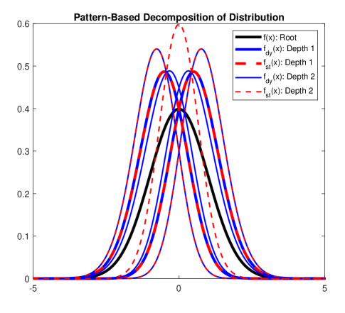
Figure 1: p.d.f.s of the pattern-based decomposed samples of standard normal time series (for both static and dynamic patterns at depth one and depth two): $f\left(x\right)$, $f^{\left(0\right)}\left(x\right)$, $f^{\left(1\right)}\left(x\right)$, $f^{\left(11\right)}\left(x\right)$, $f^{\left(10\right)}\left(x\right)$, $f^{\left(01\right)}\left(x\right)$ and $f^{\left(00\right)}\left(x\right)$.

IV Pattern-Based Estimation Model

So far we have assumed i.i.d. samples, in which for any $m\in\mathbb{N}$ such that $m<i$ we have $\Pr\left(x_{i}<x_{i-m}\right)=\Pr\left(x_{i}>x_{i-m}\right)=\frac{1}{2}$. This leads to a symmetric decomposition of the distributions of interest. Note that in many real-world applications such symmetric and i.i.d. assumptions are not valid, especially in finite time series. In fact, such asymmetry may be learned and used for prediction, estimation and compression. In this paper, we only focus on estimation. From now on, by “pattern” we only mean dynamic pattern.

Consider the autoregressive time series $x_{i}$, $i=1,2,\ldots$, satisfying $x_{i+1}=x_{i}+d_{i+1}$ where $d_{i}\sim\mathcal{N}\left(0,\sigma^{2}\right)$ is assumed to be i.i.d. and $x_{0}=\mu$. The $x_{i}$s are dependent but identically distributed (d.i.d.), and given $x_{i}$ we have $x_{i+1}\sim\mathcal{N}\left(x_{i},\sigma^{2}\right)$. Due to the asymmetric patterns in time series, instead of the model $x_{i+1}=x_{i}+d_{i+1}$ we use $x_{i+1}=x_{i}+\left(-1\right)^{q_{i+1}}\left|d_{i+1}\right|$ where $q_{i}\in\left\{0,1\right\}$ and $d_{i}\sim\mathcal{N}\left(0,\sigma^{2}\right)$. Considering depth $D$ and given a pattern $B^{\left(D-1\right)}=b_{1}b_{2}\cdots b_{D-1}$, the estimation (or forecast as considered in [10, 11]) of the next sample is $\widehat{x_{i+1}}=x_{i}+\left(-1\right)^{\widehat{q_{i+1}}}\left|\widehat{d_{i+1}}\right|$ where

$$\widehat{q_{i+1}} =\begin{cases}0,&p_{i+1}^{\left(1\right)}>p_{i+1}^{\left(0\right)};\\ 1,&\textrm{o.w.};\end{cases}$$

$$p_{i+1}^{\left(1\right)} =\Pr\left(x_{i+1}>x_{i}\biggl{|}B_{dy}^{\left(D-1\right)}\left(i\right)\right),$$

$$p_{i+1}^{\left(0\right)} =1-p_{i+1}^{\left(1\right)},$$

where $B_{dy}^{\left(D-1\right)}\left(i\right)=\bigcap_{n=i-D+2}^{i}\left\{x_{n}\overset{b_{-n+i+1}}{\lessgtr}x_{n-1}\right\}$ and

$$\widehat{d_{i+1}} =\begin{cases}\frac{1}{\left|S_{i+1}^{\left(1\right)}\right|}\sum_{x_{k}\in S_{i+1}^{\left(1\right)}}\left(x_{k}-x_{k-1}\right),&p_{i+1}^{\left(1\right)}>p_{i+1}^{\left(0\right)};\\ \frac{1}{\left|S_{i+1}^{\left(0\right)}\right|}\sum_{x_{k}\in S_{i+1}^{\left(0\right)}}\left(x_{k}-x_{k-1}\right),&\textrm{o.w.};\end{cases}$$

where $S_{i+1}^{\left(1\right)}=\left\{x_{k}\biggl{|}1\leq k\leq i,\>x_{k}>x_{k-1},B_{dy}^{\left(D-1\right)}\left(k\right)\right\}$ and $S_{i+1}^{\left(0\right)}=\left\{x_{k}\biggl{|}1\leq k\leq i,\>x_{k}\leq x_{k-1},B_{dy}^{\left(D-1\right)}\left(k\right)\right\}$. Note that such an estimation comes down to two decisions: 1) Deciding $x_{i}\overset{\widehat{q_{i+1}}}{\lessgtr}x_{i+1}$ by comparing $p_{i+1}^{\left(1\right)}$ and $p_{i+1}^{\left(0\right)}$ (where $p_{i+1}^{\left(1\right)}$ and $p_{i+1}^{\left(0\right)}$ are calculated using the results of Theorem 2 for i.i.d. case, or calculated empirically for non-i.i.d. cases), 2) Calculating the change value $\widehat{d_{i+1}}$ by averaging the change values for the samples that had the same pattern $\bigcap\left\{x_{i}\overset{\widehat{q_{i+1}}}{\lessgtr}x_{i+1},B_{dy}^{\left(D-1\right)}\left(i\right)\right\}$.

V Experiment

In this section, we apply the proposed estimator on a synthetic time series, known as Mackey-Glass [20], as well as real-world time series of heart rate data. In these experiments, first an empty binary-structured tree is created based on a (predetermined) depth, then as samples of the time series are used iteratively to fill out the tree based on the patterns, $p_{i+1}^{\left(1\right)}$ and $p_{i+1}^{\left(0\right)}$ are updated and the next sample is also estimated using the samples and patterns that have already been seen, and finally sample-wise estimation error is calculated. Algorithm 1 summarized the step-by-step procedure. We compare the estimation results with linear prediction and an adapted version of the pattern-based forecasting method proposed in [11]. One of reasons for such an adaptation is that, the proposed method in [11] needs historical data, but in our online setting “historical” data becomes available iteratively as we see more data samples.

While it’s not of our immediate interest and is subject of an ongoing work, such a pattern tree can also be used in machine learning framework, i.e. a training time series can be used to fill a pattern tree, and then the filled tree can be used in prediction/estimation of a test time series.

Algorithm 1 Pattern Tree algorithms (Note that each pattern corresponds to a path in binary-structured tree).

• Inputs:

$D_{max}$: The Predetermined maximum depth of tree
$x$: Time Series Data

1:procedure Main

2:     PT = Create($D_{max}$)

3:     PT = PT.SetPattern($x(1:D_{max})$)

4:     for $i=D_{max}+1:End$ do

5:         PT = PT.Update($i,x(i)$)

6:         $\widehat{x}(i+1)$ = PT.Estimate      

1:procedure Create($D_{max}$) $\triangleright$ Create an empty tree

2:     $n=2^{(D_{max}+1)}-1$ $\triangleright$ Total number of nodes

3:     $I=1:n$ $\triangleright$ Index of nodes

4:     $Pattern=[\>]$ $\triangleright$ Vector of size $D_{max}$

5:     $TS=[\>]$ $\triangleright$ To record the time series

1:procedure SetPattern($x$) $\triangleright$ Set the initial pattern

2:     for $i=2:D_{max}$ do

3:         if $x(i)>x(i-1)$ then

4:              $Pattern(i-1)=1$

5:         else

6:              $Pattern(i-1)=0$               

7:     $TS=x$

1:procedure Update($i,x$)

2:     if $x>TS(End)$ then

3:         update $Pattern=[Pattern\quad 1]$

4:     else

5:         update $Pattern=[Pattern\quad 0]$      

6:     calculate Path using Pattern

7:     for $d=1:D_{max}$ do

8:         add $i$ to the node $I(d,path)$      

9:     update $Pattern=Pattern(2:D_{max})$

10:     update $TS=[TS\quad x]$

1:procedure Estimate

2:     $Pattern0=[Pattern\quad 0]$

3:     $Pattern1=[Pattern\quad 1]$

4:     calculate Path0 using Pattern0

5:     calculate Path1 using Pattern1

6:     $d=D_{max}$, $J=[\>]$

7:     while $d\geq 1$ and $J=[\>]$ do

8:         if $P(Pattern1)>P(Pattern0)$ then

9:              $J=$ indexes in node $I(d,path1)$

10:              $\widehat{x}=TS(End)+mean(TS(J)-TS(J-1))$

11:         else if $P(Pattern0)>P(Pattern1)$ then

12:              $J=$ indexes in node $I(d,path0)$

13:              $\widehat{x}=TS(End)-mean(TS(J)-TS(J-1))$          

14:         $d=d-1$      

15:     return $\widehat{x}$

V-A Mackey-Glass

The Mackey-Glass time series is a nonlinear time delay differential equation and was originally introduced to represent the appearance of complex dynamic in physiological control systems. It is derived by finite difference discretization of the nonlinear differential equation $\frac{dx\left(t\right)}{dt}=-ax\left(t\right)+\frac{bx\left(t-\tau\right)}{1+x^{10}\left(t-\tau\right)},\>t\geq 0$, where $a$, $b$ and $\tau$ are constants. We generated 10000 samples of this time series with $a=0.2$, $b=0.1$ and $\tau=17$ and followed the steps described in Section V. Table I summarizes the comparison between our proposed pattern tree method, the pattern-based forecasting method proposed in [11] and linear prediction in terms of estimation mean squared error (MSE). As can be seen, our proposed method outperforms others.

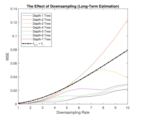
Figure 2: The effect of time series sampling frequency on estimation error for pattern trees of various depths.

In the second experiment using Mackey-Glass time series, we analyze the effect of downsampling. Fig. 2 shows the estimation MSE versus downsampling rate. As expected, estimation using deeper pattern trees ($D\geq 3$) are more resilient to downsampling.

V-B Heart Rate Data

In the second experiment we used the heart rate time series recorded by E4 Empatica wristbands (sampling frequency for hear rate measurements of this wearable device is 1 Hz). Similar to the Mackey-Glass experiment, we used 10000 samples of recorded heart rate data and followed the steps described in Section V. As can be seen in Table I, similar to the previous experiment with Mackey-Glass time series, our proposed pattern tree method performs better than others in terms of estimation MSE.

Depth/ Order	Mackey-Glass			Heart Rate
	PT	[11]	LP	PT	[11]	LP
1	$\!\!0.0011\!\!$	$\!\!0.0012\!\!$	$\!\!0.0011\!\!$	$\!\!0.0101\!\!$	$\!\!0.0114\!\!$	$\!\!0.2528\!\!$
2	$\!\!3.95\!\!\times\!\!10^{-4}\!\!$	$\!\!6.15\!\!\times\!\!10^{-4}\!\!$	$\!\!0.0081\!\!$	$\!\!0.0057\!\!$	$\!\!0.0104\!\!$	$\!\!0.3915\!\!$
3	$\!\!3.85\!\!\times\!\!10^{-4}\!\!$	$\!\!6.17\!\!\times\!\!10^{-4}\!\!$	$\!\!0.0153\!\!$	$\!\!0.0055\!\!$	$\!\!0.0103\!\!$	$\!\!0.3257\!\!$
4	$\!\!3.84\!\!\times\!\!10^{-4}\!\!$	$\!\!6.11\!\!\times\!\!10^{-4}\!\!$	$\!\!0.0239\!\!$	$\!\!0.0054\!\!$	$\!\!0.0103\!\!$	$\!\!0.3279\!\!$
5	$\!\!3.81\!\!\times\!\!10^{-4}\!\!$	$\!\!5.95\!\!\times\!\!10^{-4}\!\!$	$\!\!0.0336\!\!$	$\!\!0.0054\!\!$	$\!\!0.0102\!\!$	$\!\!0.3674\!\!$

Table I: Comparison of mean squared error of estimation using our proposed pattern tree (PT) method, linear prediction (LP) and an adapted version of the pattern-based forecasting method proposed in [11] for various depths/orders.

References

- [1] E. Sabeti and A. Høst-Madsen, “Data discovery and anomaly detection using atypicality for real-valued data,” Entropy, vol. 21, no. 3, p. 219, 2019.
- [2] A. Høst-Madsen, E. Sabeti, and C. Walton, “Data discovery and anomaly detection using atypicality: Theory,” IEEE Transactions on Information Theory, 2019.
- [3] S. R. Islam, D. Kwak, M. H. Kabir, M. Hossain, and K.-S. Kwak, “The internet of things for health care: a comprehensive survey,” IEEE Access, vol. 3, pp. 678–708, 2015.
- [4] L. Breiman, Classification and regression trees. Routledge, 2017.
- [5] F.-L. Chung, T.-C. Fu, V. Ng, and R. W. Luk, “An evolutionary approach to pattern-based time series segmentation,” IEEE transactions on evolutionary computation, vol. 8, no. 5, pp. 471–489, 2004.
- [6] G. Ouyang, C. Dang, D. A. Richards, and X. Li, “Ordinal pattern based similarity analysis for eeg recordings,” Clinical Neurophysiology, vol. 121, no. 5, pp. 694–703, 2010.
- [7] X. Liu, Z. Ni, D. Yuan, Y. Jiang, Z. Wu, J. Chen, and Y. Yang, “A novel statistical time-series pattern based interval forecasting strategy for activity durations in workflow systems,” Journal of Systems and Software, vol. 84, no. 3, pp. 354–376, 2011.
- [8] D. J. Berndt and J. Clifford, “Using dynamic time warping to find patterns in time series.” in KDD workshop, vol. 10, no. 16. Seattle, WA, 1994, pp. 359–370.
- [9] T.-c. Fu, F.-l. Chung, R. Luk, and C.-m. Ng, “Stock time series pattern matching: Template-based vs. rule-based approaches,” Engineering Applications of Artificial Intelligence, vol. 20, no. 3, pp. 347–364, 2007.
- [10] S. Alvisi, M. Franchini, and A. Marinelli, “A short-term, pattern-based model for water-demand forecasting,” Journal of hydroinformatics, vol. 9, no. 1, pp. 39–50, 2007.
- [11] F. M. Alvarez, A. Troncoso, J. C. Riquelme, and J. S. A. Ruiz, “Energy time series forecasting based on pattern sequence similarity,” IEEE Transactions on Knowledge and Data Engineering, vol. 23, no. 8, pp. 1230–1243, 2010.
- [12] W.-G. Teng, M.-S. Chen, and P. S. Yu, “A regression-based temporal pattern mining scheme for data streams,” in Proceedings of the 29th international conference on Very large data bases-Volume 29. VLDB Endowment, 2003, pp. 93–104.
- [13] Q. Hu, P. Su, D. Yu, and J. Liu, “Pattern-based wind speed prediction based on generalized principal component analysis,” IEEE Transactions on Sustainable Energy, vol. 5, no. 3, pp. 866–874, 2014.
- [14] S. S. Kozat, A. C. Singer, and G. C. Zeitler, “Universal piecewise linear prediction via context trees,” IEEE Transactions on Signal Processing, vol. 55, no. 7, pp. 3730–3745, 2007.
- [15] F. Willems, Y. Shtarkov, and T. Tjalkens, “Reflections on "the context tree weighting method: Basic properties",” Newsletter of the IEEE Information Theory Society, vol. 47, no. 1, 1997.
- [16] F. M. J. Willems, Y. Shtarkov, and T. Tjalkens, “The context-tree weighting method: basic properties,” Information Theory, IEEE Transactions on, vol. 41, no. 3, pp. 653–664, 1995.
- [17] F. Willems, “The context-tree weighting method: extensions,” Information Theory, IEEE Transactions on, vol. 44, no. 2, pp. 792–798, Mar 1998.
- [18] N. Eugene, C. Lee, and F. Famoye, “Beta-normal distribution and its applications,” Communications in Statistics-Theory and methods, vol. 31, no. 4, pp. 497–512, 2002.
- [19] A. K. Gupta and S. Nadarajah, “On the moments of the beta normal distribution,” Communications in Statistics-Theory and Methods, vol. 33, no. 1, pp. 1–13, 2005.
- [20] M. C. Mackey and L. Glass, “Oscillation and chaos in physiological control systems,” Science, vol. 197, no. 4300, pp. 287–289, 1977.