Classical Hamiltonian Time Crystals – General Theory And Simple Examples

Abstract

We focus on a Hamiltonian system with a continuous symmetry, and dynamics that takes place on a presymplectic manifold. We explain how the symmetry can become spontaneously broken by a time crystal, that we define as the minimum of the available mechanical free energy that is simultaneously a time dependent solution of Hamilton’s equation. The mathematical description of such a timecrystalline spontaneous symmetry breaking builds on concepts of equivariant Morse theory in the space of Hamiltonian flows. As an example we analyze a general family of timecrystalline Hamiltonians that is designed to model polygonal, piecewise linear closed strings. The vertices correspond to the locations of pointlike interaction centers; the string is akin a chain of atoms, that are joined together by covalent bonds, modeled by the links of the string. We argue that the timecrystalline character of the string can be affected by its topology. For this we show that a knotty string is usually more timecrystalline than a string with no self-entanglement. We also reveal a relation between phase space topology and the occurrence of timecrystalline dynamics. For this we show that in the case of three point particles, the presence of a time crystal can relate to a Dirac monopole that resides in the phase space. Our results propose that physical examples of Hamiltonian time crystals can be realized in terms of closed, knotted molecular rings.

Keywords: Time crystals, Hamiltonian dynamics, Presymplectic geometry, Equivariant Morse theory

1 Introduction

Time crystals were originally introduced by Wilczek and Shapere [1, 2, 3, 4]. They proposed that a time crystal is a minimum energy configuration, that is also time dependent. As a consequence a time crystal breaks time translation invariance spontaneously, in the same manner how an ordinary crystal breaks space translation symmetry. Soon afterwards it was argued that time crystals can not exist, in the Hamiltonian context [5, 6]. But recently explicit examples of Hamiltonian time crystals have been constructed [7, 8, 9]. A general framework has also been developed [9], it identifies a set of conditions that are sufficient for the existence of a Hamiltonian time crystal: Time crystalline dynamics can take place provided Hamilton’s equation has symmetries that give rise to conserved Noether charges. A time crystal breaks the symmetry spontaneously, including time translation symmetry: A time crystal is simultaneously both a minimum of the energy and a time periodic trajectory, that is generated by a definite linear combination of the conserved charges. For this kind of timecrystalline spontaneous symmetry breaking to occur the phase space needs to have a presymplectic structure [14]. The proper mathematical framework engages equivariant Morse theory in the space of closed Hamiltonian trajectories [10, 11, 12, 13].

Here we explain in detail the origin and character of timecrystalline Hamiltonian dynamics; the article is largely a survey of our original work, published in [7, 8, 9]. We first explain why conserved Noether charges are necessary for a Hamiltonian time crystal to exist. We describe how a time crystal spontaneously breaks the symmetry group of Noether charges into an abelian subgroup that generates periodic timecrystalline motion. As an example we analyze in detail a general family of Hamiltonians [7] that support timecrystalline dynamics. The Hamiltonians are designed to model the dynamics of piecewise linear, polygonal strings: For a physical example, the timecrystalline Hamiltonian functions we consider appear often as energy functions in the context of coarse grained models of molecular chains [15]. The pertinent conserved quantity that gives rise to the timecrystalline dynamics in our Hamiltonian description simply states the geometric actuality, that the chain forms a closed string. We then bring up that a closed ring is an elemental example of a string with a knot; a simple closed string is known as the unknot. This motivates us to consider more complex entangled structures, and we proceed to show that when the knottiness of a closed string increases its timecrystalline qualities are usually enhanced. As an example we analyze in detail a closed polygonal string that forms a trefoil knot.

We then inquire about the microscopic origin of timecrystalline dynamics, at the level of the phase space topology. Our starting point is the well known result in geometric mechanics that when a deformable body contains at least three independently movable components, its vibrational and rotational motions are no longer separable [16, 17, 18, 19, 20]. Even with no net angular momentum, small local vibrations can cause a global rotation of the entire body. We argue that this relation between vibrations and rotations can provide an explanation of effective timecrystalline dynamics, in the case of a molecular ring. Thus our results propose that ring molecules, and in particular those that support a knot, are good candidates for actual physical examples of Hamiltonian time crystals.

2 Theory of Hamiltonian time crystals

Initially it was thought that there can not be any energy conserving, Hamiltonian time crystals [5, 6]. This is the conclusion that one arrives at, when one looks at the textbook Hamilton’s equation

$$\eqalign{\frac{dq^{a}}{dt}=\{q^{a},H\}=\frac{\partial H}{\partial p^{a}}\cr\frac{dp^{a}}{dt}=\{p^{a},H\}=-\frac{\partial H}{\partial q^{a}}}$$ (1)

Suppose that ($q^{a},p^{a}$) are (possibly local) coordinates on a phase space that is a compact closed manifold. Then a minimum of the Hamiltonian energy function $H(q,p)$ is also its critical point, so that at the energy minimum the right hand sides of (1) vanish. As a consequence the left hand sides must also vanish, and we immediately conclude that a minimum of $H$ can only be a time independent solution of Hamilton’s equation. In particular, we conclude that there are no Hamiltonian time crystals.

However, there is a way to go around this argument, and we now explain how it goes. We start with Hamilton’s equation that is defined on a $2N$ dimensional phase space which is a symplectic manifold $\mathcal{M}$; for a background on geometric mechanics see for example [14]. On a symplectic manifold there is always a closed and non-degenerate two-form $\Omega$,

$$\eqalign{&\Omega=\Omega_{ab}d\phi^{a}\wedge d\phi^{b}\cr d&\Omega=0}$$ (2)

The $\phi^{a}$ ($a=1,...,2N$) are generic local coordinates on the manifold $\mathcal{M}$. Hamilton’s equation is

$$\Omega_{ab}\frac{d\phi^{b}}{dt}=\partial_{a}H$$ (3)

where the Hamiltonian $H(\phi)$ is a smooth real valued function that is supported by $\mathcal{M}$. A solution of Hamilton’s equation (3) describes a trajectory $\phi^{a}(t)$ on the manifold $\mathcal{M}$. The trajectories are non-intersecting, they are uniquely defined by the initial values $\phi^{a}(0)$. The inverse of the matrix $\Omega_{ab}$ determines the Poisson brackets on $\mathcal{M}$,

$$\{\phi^{a},\phi^{b}\}=\Omega^{ab}(\phi)$$ (4)

and we can use the Poisson brackets to write Hamilton’s equation (3) as follows,

$$\frac{d\phi^{a}}{dt}\ =\ \{\phi^{a},H\}\ =\ \Omega^{ab}\partial_{b}H$$ (5)

A time crystal would be a solution of Hamilton’s equation (5) that has both a non-trivial $t$-dependence, and is also a minimum of the Hamiltonian energy function $H(\phi)$. We now show that despite the No-Go argument of (1), such Hamiltonian time crystals do exist provided a set of conditions is satisfied.

For clarity we shall only search for genuine time crystals, those that are periodic functions of time $\phi^{a}(t+T)=\phi^{a}(t)$ for some finite non-vanishing $T$. Thus a time crystal would spontaneously break continuous time translation symmetry into a discrete group of time translations. But we note that depending on $H$ there might also be timecrystalline solutions that are non-periodic in $T$. They also break time translation symmetry, their properties can be analyzed similarly.

Darboux theorem states that on a symplectic manifold we can always find a local coordinate transformation that sends the $\phi^{a}$ to the canonical momenta and coordinates ($q^{a},p^{a}$) with their standard canonical Poisson brackets. In such Darboux coordinates Hamilton’s equation acquires the textbook form (1) and without any additional input, the simple No-Go argument that is based on (1) is valid and excludes timecrystalline solutions of (3). Thus, to construct timecrystalline Hamiltonian dynamics, we need to proceed beyond plain symplectic geometry. Such a more general framework is presymplectic geometry. A presymplectic manifold is simply a manifold with a closed two-form. Presymplectic structure can be encountered, even in a symplectic context, for example when Hamilton’s equation is subject to contraints, or when it supports continuous symmetries. On a presymplectic manifold the No-Go theorems [5, 6] no longer need to be applicable. Time crystals can exist, and we now explain how this can take place, in the case of Hamilton’s equation with continuous symmetries [9].

We start with a Hamiltonian function $H(\phi)$ that describes dynamics on a $2N$ dimensional symplectic manifold $\mathcal{M}$; our presymplectic structure emerges in the context of standard symplectic geometry. Thus we start with a non-singular symplectic two-form with components $\Omega_{ab}$. Its inverse matrix $\Omega^{ab}$ determines the Poisson bracket (4) that gives rise to Hamilton’s equation (5).

We now assume that, in addition, the Hamiltonian has a continuous symmetry. According to Noether’s theorem a continuous symmetry gives rise to a conservation law. We denote the ensuing conserved charges $G_{i}(\phi)$ with $i=1,...,n\leq N$. The Poisson brackets of the conserved charges with the Hamiltonian vanish,

$$\frac{dG_{i}}{dt}\ =\ \{H,G_{i}\}=\Omega^{ab}\partial_{a}H\partial_{b}G_{i}=0$$ (6)

The Poisson brackets of the $G_{i}$ closes, and coincides with the Lie algebra of the symmetry group,

$$\{G_{i},G_{j}\}={f_{ij}}^{k}G_{k}$$ (7)

We assume that there is no spontaneous symmetry breaking, in the usual fashion. Instead we proceed to describe how the symmetry becomes spontaneously broken, by a time crystal.

We introduce the numerical values of the conserved charges

$$G_{i}\left(\phi(0)\right)=g_{i}$$ (8)

They are specified by the initial conditions $\phi^{a}(0)$ of Hamilton’s equation. The preimages of $g_{i}$ foliate the symplectic manifold $\mathcal{M}$ into leaves that are specified by the conditions

$$\mathcal{G}_{i}^{g}(\phi)\ =\ G_{i}(\phi)-g_{i}=0$$ (9)

Each regular value of $g_{i}$ defines a submanifold $\mathcal{M}_{g}$ of the symplectic manifold $\mathcal{M}$. Notably the Poisson brackets of the (9) do not close, but instead we obtain

$$\{\mathcal{G}^{g}_{i},\mathcal{G}^{g}_{j}\}={f_{ij}}^{k}\,\mathcal{G}^{g}_{k}+{f_{ij}}^{k}g_{k}$$ (10)

where the right hand side defines a $n\times n$ matrix

$$\gamma_{ij}(g)={f_{ij}}^{k}g_{k}$$ (11)

In general this matrix is singular. We assume that its image has a dimension $s\leq n$; its kernel then has a dimension $(n-s)$. In general these dimensions depend on the numerical values $\{g_{i}\}$.

For given, fixed values $g_{i}$ we restrict the non-degenerate symplectic two-form $\Omega$ of $\mathcal{M}$ to the corresponding submanifold $\mathcal{M}_{g}$ and we denote the restriction by

$$\Omega_{|_{\mathcal{M}_{g}}}\ \equiv\ \omega^{g}=\omega^{g}(\phi)_{ab}d\phi^{a}\wedge d\phi^{b}$$ (12)

The two-form $\omega^{g}$ is closed, but in general the ensuing matrix $\omega^{g}_{ab}$ is degenerate. Its kernel has dimension ($n-s$) i.e. the kernel dimension is equal to that of the matrix (11). Thus, whenever $n-s\not=0$ the submanifold $\mathcal{M}_{g}$ that we equip with the closed two-form (12), is not a symplectic manifold but a presymplectic manifold [14].

We shall assume that the physical system of interest has the property, that all those values $\{g_{i}\}$ that describe the actual physical scenario always have $n-s\not=0$. The two-form $\omega^{g}$ then determines Hamiltonian dynamics that takes place on a presymplectic submanifold $\mathcal{M}_{g}$ of the initial symplectic manifold $\mathcal{M}$. Since the No-Go theorem [5, 6] assumes that the Hamiltonian dynamics takes place on a symplectic manifold, it no longer applies to dynamics that takes place on $\mathcal{M}_{g}$ and we can start searching for a timecrystalline solution of Hamilton’s equation.

We first need to locate the minimum value of the Hamiltonian $H(\phi)$ on the submanifolds $\mathcal{M}_{g}$. For this we use the method of Lagrange multipliers: We introduce $n$ Lagrange multipliers $\lambda^{i}$ and we extend the Hamiltonian $H(\phi)$ as follows,

$$H\to H_{\lambda}=H+\lambda^{i}(G_{i}-g_{i})$$ (13)

The Lagrange multiplier theorem [14] states that on a submanifold $\mathcal{M}_{g}$ the minimum value $\phi^{a}_{cr}$ of the Hamiltonian $H(\phi)$ coincides with a critical point ($\phi^{a}_{cr},\lambda_{cr}^{i}$) of the extended Hamiltonian $H_{\lambda}(\phi)$. Thus we can locate the minimum value of $H(\phi)$ on $\mathcal{M}_{g}$ by solving the equations

$$\left\{\eqalign{\frac{\partial H}{\partial\phi^{a}}_{|\phi_{cr}}&=-\lambda_{cr}^{i}\frac{\partial G_{i}}{\partial\phi^{a}}_{|\phi_{cr}}\cr G_{i}(\phi_{cr})&=g_{i}}\right.$$ (14)

Accordingly, our search of a time crystal proceeds as follows:

$\bullet~{}$ We first use the equations (14) and locate the minimum $\phi^{a}_{cr}$ of $H(\phi)$ on $\mathcal{M}_{g}$, for all those values $\{g_{i}\}$ of the conserved charges that correspond to the physical scenario that we consider.

$\bullet~{}$ We then proceed and solve from (14) the corresponding values $\lambda^{i}_{cr}$ in terms of $\phi^{a}_{cr}$.

$\bullet~{}$ Whenever $\lambda^{i}_{cr}(\phi_{cr})\not=0$ we have a time crystal: The minimum energy solution $\phi^{a}_{cr}$ serves as an initial value to the time crystalline solution of Hamilton’s equation (5). Thus, in the case of a time crystal we can use (14) to rewrite Hamilton’s equation (5) as follows,

$$\eqalign{\frac{d\phi^{a}}{dt}&=\ -\Omega^{ab}\lambda^{i}_{cr}\frac{\partial G_{i}}{\partial\phi^{b}}\not=0\cr\phi^{a}(0)&=\ \phi^{a}_{cr}}$$ (15)

The existence of a time crystal is a manifestation of spontaneous symmetry breaking, but in a time dependent context: The equation (15) states that a time crystal is simply a time dependent minimal energy symmetry transformation that is generated by a subgroup of the full symmetry group. This subgroup is spanned by the following linear combination of the conserved Noether charges,

$$G_{\lambda}(\phi)\equiv\lambda^{i}_{cr}G_{i}(\phi)$$ (16)

Accordingly the time crystal breaks the full symmetry group (7) of the Hamiltonian into the abelian U(1) subgroup (16). Note that both $H(\phi)$ and $G_{i}(\phi)$ are by construction $t$-independent along any Hamiltonian trajectory. Thus the Lagrange multipliers $\lambda^{i}_{cr}$ are time independent. They depend only on the initial configuration $\phi^{a}_{cr}$, as determined by the equation (14).

We conclude this Section and mention that our construction of Hamiltonian time crystals can be rigorously formulated and analysed using the methods of equivariant Morse theory [10, 11, 12, 13] in the space of loops on a presymplectic manifold.

3 Family Of Timecrystalline Hamiltonians

As an example of timecrystalline Hamiltonian dynamics we consider a polygonal string. The string is made of linear links that connect pointlike interaction centers, that are located at its $N+1$ vertices including the end points [7].

In a physical application the interaction centers can model atoms. The links of the string are then the covalent bonds. However, at this point we do not propose to describe any specific material system: In any physical application to a stringlike molecule, the Hamiltonian approach that we develop should be interpreted in terms of an effective theory description. An effective theory aims to describe a complex physical system in terms of a reduced set of variables. The reduced variables should provide an adequate description of the physical phenomena, at length and time scales that are large in comparison to the characteristic fundamental level (atomic) length and time scales. In many circumstances, when there is a separation of scales, such an effective theory description that builds on a reduced set of variables can be treated as a conventional dynamical system in its own right. In many cases the dynamics can be governed by an energy conserving effective Hamiltonian description, in a useful approximation.

The vertices of the string have coordinates $\mathbf{x}_{i}$ ($i=1,...,N+1$) and the links are the vectors

$$\mathbf{n}_{i}\ =\ \mathbf{x}_{i+1}-\mathbf{x}_{i}\ \ \ \ \ (i=1,...,N)$$ (17)

The $N$ vectors $\mathbf{n}_{i}$ are our dynamical degrees of freedom, and we impose on them the following Lie-Poisson bracket

$$\{n^{a}_{i},n^{b}_{j}\}=\delta_{ij}\epsilon^{abc}n^{c}_{i}$$ (18)

The variables $\mathbf{n}_{i}$ together with their Lie-Poisson brackets are designed to generate any kind of local motion of the vertices, except for stretching and shrinking of the links. Indeed, since

$$\{n^{a}_{i},\mathbf{n}_{j}\cdot\mathbf{n}_{j}\}=0$$

for all $i,j$ the bracket preserves the length of $\mathbf{n}_{i}$ independently of the Hamiltonian function. For convenience we set all $|\mathbf{r}_{i+1}-\mathbf{r}_{i}|=1$ in the following.

We note that a Lie-Poisson bracket simply describes how a Poisson manifold i.e. a manifold that is equipped with a Poisson bracket, foliates into symplectic leaves. Here, for each link $i$ the Poisson manifold is $\mathbb{R}^{3}$ and the leaves are the two-spheres $\mathbb{S}^{2}$ with radii $r_{i}=|\mathbf{x}_{i+1}-\mathbf{x}_{i}|$. We can always introduce local Darboux variables ($p_{i},q_{i}$) with their standard Poisson brackets, simply by defining

$$\mathbf{n}\ =\ \left(\eqalign{n^{1}\cr n^{2}\cr n^{3}}\right)\ =\ r\left(\eqalign{\cos\varphi\sin\vartheta\cr\sin\varphi\sin\vartheta\cr\ \ \ \cos\vartheta}\right)$$ (19)

The Lie-Poisson bracket (18) then reduces to

$$\{\cos\vartheta,\varphi\}=-\frac{1}{r}$$

and thus ($\cos\vartheta,\varphi$)$\sim$($p,q$) are Darboux coordinates, but instead of ($\vartheta_{i},\varphi_{i}$) in the present case of a piecewise linear string we find it more convenient to proceed in terms of the Lie-Poisson variables $\mathbf{n}_{i}$ due to their immediate geometric interpretation.

The Lie-Poisson bracket (18) gives rise to the following Hamiltonian equation

$$\frac{\partial\mathbf{n}_{i}}{\partial t}\ =\ \{\mathbf{n}_{i},H(\mathbf{n})\}\ =\ -\mathbf{n}_{i}\times\frac{\partial H}{\partial\mathbf{n}_{i}}$$ (20)

To introduce the conserved charges (6), (7) and to specify the details of the Hamiltonian a posteriori, we start with the end-to-end distance

$$\mathbf{G}\ =\ \sum\limits^{N}_{i=1}\,\mathbf{n}_{i}\ =\ \mathbf{x}_{N+1}-\mathbf{x}_{1}$$ (21)

The components satisfy

$$\{G^{a},G^{b}\}=\epsilon^{abc}G^{c}$$ (22)

Here we focus solely on Hamiltonians that preserve the end-to-end distance

$$\{H(\mathbf{n}),\mathbf{G}\}\ =\ 0$$ (23)

Furthermore, in the following we shall always assume that the string is closed so that

$$g_{i}\sim\mathbf{x}_{N+1}-\mathbf{x}_{1}=0$$

For (9) we then have

$$\mathbf{G}\ =\ \sum\limits^{N}_{i=1}\,\mathbf{n}_{i}=0$$ (24)

and the Poisson bracket (10) of the corresponding $\mathcal{G}^{a}_{i}$ closes and coincides with (22). Since the matrix (11) now vanishes the pertinent kernel of $\gamma_{ij}$ is three dimensional and in particular it does not vanish: In the case of a closed string, the phase space is presymplectic and we are interested in the ensuing Hamiltonian dynamics.

We search for a timecrystalline solution of (20), (24) using the relevant equation (14). For this we introduce a Lagrange multiplier ${\boldsymbol{\lambda}}$ and look for extrema of

$$H_{\boldsymbol{\lambda}}=H(\mathbf{n})+{\boldsymbol{\lambda}}\cdot\mathbf{G}$$ (25)

The time evolution of the time crystal (15) is then simply

$$\frac{\partial\mathbf{n}_{i}}{\partial t}=-{\boldsymbol{\lambda}}_{cr}\times\mathbf{n}_{i}$$ (26)

with the initial condition

$$\mathbf{n}_{i}(t=0)=\mathbf{n}_{i,cr}$$

where $\mathbf{n}_{i,cr}$ is the critical point of (25) that corresponds to minimal $H(\mathbf{n})$ value, in the case of a closed string, and

$${\boldsymbol{\lambda}}_{cr}=-\frac{\partial H}{\partial\mathbf{n}_{i}}_{|\mathbf{n}_{cr}}$$ (27)

Thus, whenever (27) is nonvanishing we have a time crystal.

The Lie-Poisson bracket makes the search for a fixed point of (25) straightforward: We simply extend Hamilton’s equation (20) into

$$\frac{\partial\mathbf{n}_{i}}{\partial t}=-\mathbf{n}_{i}\times\frac{\partial H_{\boldsymbol{\lambda}}}{\partial\mathbf{n}_{i}}+\mu\,\mathbf{n}_{i}\times(\mathbf{n}_{i}\times\frac{\partial H_{\boldsymbol{\lambda}}}{\partial\mathbf{n}_{i}})$$ (28)

where $\mu>0$ is a parameter; note that (28) also preserves the bond lengths $\mathbf{n}_{i}\cdot\mathbf{n}_{i}$. From this we derive

$$\frac{dH_{\boldsymbol{\lambda}}}{dt}=-\frac{\mu}{1+\mu^{2}}\sum\limits_{i=1}^{N}\left|\frac{d\mathbf{n}_{i}}{dt}\right|^{2}\ \leq\ 0$$ (29)

Thus, whenever $\mu>0$ the time evolution of (29) proceeds towards decreasing values of $H_{\boldsymbol{\lambda}}$ and the flow (29) continues until it meets a critical point value ($\mathbf{n}_{i,cr}\,,{\boldsymbol{\lambda}}_{cr}$).

The present observations can be readily developed into a numerical algorithm that we can employ to systematically locate the critical point ($\mathbf{n}_{i,cr}\,,{\boldsymbol{\lambda}}_{cr}$) for which the Hamiltonian function $H(\mathbf{n})$ has a minimal value.

4 Existence And Simple Examples

We now present simple examples; the examples show by explicit construction, that Hamiltonian time crystals do indeed exist [7].

Our first example has a Hamiltonian function of the form

$${H_{1}}\ =\ -\sum\limits_{i=1}^{N}a_{i}\,\mathbf{n}_{i}\cdot\mathbf{n}_{i+1}$$ (30)

Clearly, its Poisson bracket with (21) vanishes. We start with $N=3$, with (24) we have $\mathbf{n}_{4}\equiv\mathbf{n}_{1}$ so that the string is closed and its vertices $\mathbf{x}_{1},\,\mathbf{x}_{2}$ and $\mathbf{x}_{3}$ are the corners of an equilateral triangle. The energy function can only have one value but its derivatives are nonvanishing, and the Lie-Poisson bracket (18) gives Hamilton’s equation

$$\cases{\frac{d\mathbf{n}_{1}}{dt}=\mathbf{n}_{1}\times(a_{1}\mathbf{n}_{2}+a_{3}\mathbf{n}_{3})\\ \frac{d\mathbf{n}_{2}}{dt}=\mathbf{n}_{2}\times(a_{2}\mathbf{n}_{3}+a_{1}\mathbf{n}_{1})\\ \frac{d\mathbf{n}_{3}}{dt}=\mathbf{n}_{3}\times(a_{3}\mathbf{n}_{1}+a_{2}\mathbf{n}_{2})\\ }$$ (31)

This can be easily solved:

For $a_{1}=a_{2}=a_{3}$ we have only the time independent solution and no time crystal, the solution is an equilateral triangle at rest.

For generic values of $a_{i}$ elementary linear algebra shows that the right hand sides of equations (31) can not all vanish simultaneously. The solution which is unique up to time translation, is an equilateral timecrystalline triangle rotating around an axis that is on the plane of the triangle, goes through its center, and points to a direction that is determined by the parameters ($a_{1},a_{2},a_{3}$) as shown in Figure 1 a).

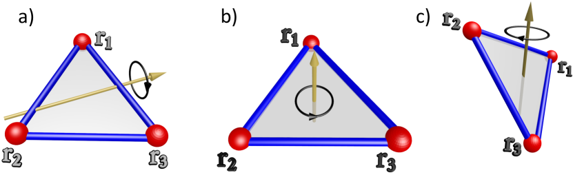
Figure 1: Figure a) For generic parameter values ($a_{1},a_{2},a_{3}$) the timecrystalline solution of equation (31) describes an equilateral triangle rotating around an axis on its plane and thru its center, with direction determined by the parameters. Figure b) For $N=3$ the time crystal of Hamiltonian (32) rotates around an axis which is normal to its plane, the direction of rotation is determined by the sign(s) of $b_{i}$. Figure c) A linear combination of the Hamiltonians (30), (32) with $N=3$ gives a equilateral triangular time crystal that rotates around a generic axis thru its center.

As another example, the following Hamiltonian

$${H_{2}}\ =\ -\sum\limits_{i=2}^{N}b_{i}\,\mathbf{n}_{i}\cdot(\mathbf{n}_{i-1}\times\mathbf{n}_{i+1})$$ (32)

also obeys (23), and for $N=3$ (so that $\mathbf{n}_{4}\equiv\mathbf{n}_{1}$) it supports a time crystal as an equilateral triangle.This time crystal rotates around its symmetric normal axis as shown in Figure 1 b).

The $N=3$ linear superposition $H_{1}+H_{2}$ supports a Hamiltonian time crystal that rotates around a generic axis which passes through the geometric center of the equilateral triangle; the direction of the rotation axis and the speed and orientation of the rotation are determined by the parameters. See Figure 1 c).

The present simple examples prove the existence of Hamiltonian time crystals. But we did not need to explicitly search for the critical points of the Hamiltonian (25); when $N=3$ the condition (24) can only be satisfied with an equilateral triangle. For more than $N=3$ vertices we first need to locate the minimal energy configuration $\mathbf{n}_{i,cr}$ and then solve for the Lagrange multiplier ${\boldsymbol{\lambda}}_{cr}$ in terms of $\mathbf{n}_{i,cr}$. For this we introduce (28). As an example we consider the Hamiltonian (32) with $N=4$, with only one non-vanishing parameter $b_{1}=-1$. The minimum energy configuration maximizes the volume that is subtended by four unit vectors such that

$$\mathbf{G}=\mathbf{n}_{1}+\mathbf{n}_{2}+\mathbf{n}_{3}+\mathbf{n}_{4}=0$$

For energy minimum the vertices are the four corners of a tetragonal disphenoid [21], its faces are isosceles triangles with edge lengths in the proportions $\sqrt{3}:\sqrt{3}:2$. Tetragonal disphenoid is a remarkable geometric object. Unlike the regular tetrahedron it tesselate spaces, and it can also be constructed by simple foldings of A4 standard paper as the side ratios of A4 are $1:\sqrt{2}$ [21, 22]. The Figure 2 shows the structure and depicts its timecrystalline rotation.

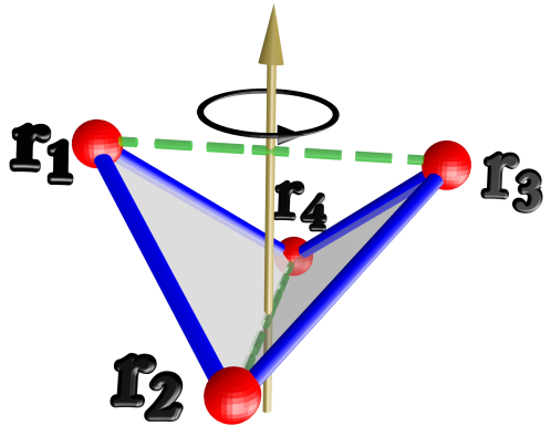
Figure 2: For $N=4$ the time crystal described by the Hamiltonian (32) is a tetragonal disphenoid that rotates around its symmetry axis; the length ratio of the two green segments to the four blue segments is $2:\sqrt{3}$. The direction of rotation is determined by the sign of $b_{i}$.

5 Topology And Time Crystals

For additional, more elaborate timecrystalline Hamiltonian functions [8] we observe that the spatial separation $\mathbf{x}_{j}-\mathbf{x}_{k}$ between any two vertices ($j,k$) along our closed string can always be presented in terms of the bond vectors $\mathbf{n}_{i}$,

$$\mathbf{x}_{k}-\mathbf{x}_{j}=\frac{1}{2}(\mathbf{n}_{j}+...+\mathbf{n}_{k-1})-\frac{1}{2}(\mathbf{n}_{k}-...-\mathbf{n}_{j-1})$$ (33)

We have here introduced a symmetrization, to account for the fact that the vertices $\mathbf{x}_{i}$ and $\mathbf{x}_{k}$ are connected in two different ways along the closed string. Consistent with (23) we can then add to the Hamiltonian any two-body interaction $U(|\mathbf{x}_{k}-\mathbf{x}_{j}|)$.

In the case of molecular modeling [15] the vertices of our string describe atoms or small molecules. They are subject to mutual two-body interactions including the electromagnetic Coulomb potential and the Lennard-Jones potential; the latter is a sum of the attractive van der Waals interaction and the repulsive Pauli exclusion interaction. In the case of charged vertices, at large distances the van der Waals interaction becomes small in comparison to the Coulomb interaction, and at short distances the Pauli repulsion dominates. Thus, for clarity, here we only consider the Coulomb and the Pauli repulsion interactions. Accordingly we introduce the following contribution to our timecrystalline Hamiltonian free energy,

$$U(\mathbf{x}_{1},...,\mathbf{x}_{N})=\frac{1}{2}\underset{i\not=j}{\sum_{i,j=1}^{N}}\frac{e_{i}e_{j}}{|\mathbf{x}_{i}-\mathbf{x}_{j}|}+\frac{1}{2}\underset{i\not=j}{\sum_{i,j=1}^{N}}\left(\frac{r_{min}}{|\mathbf{x}_{i}-\mathbf{x}_{j}|}\right)^{\!\!12}$$ (34)

Here $e_{i}$ is the electric charge at the vertex $\mathbf{x}_{i}$ and $r_{min}$ characterizes the extent of the Pauli exclusion; the Pauli exclusion prevents string self-crossing, in the case of actual molecules covalent bonds do not cross each other.

We note that a Hamiltonian function such as the linear combination of (30), (32), (34) commonly appears in coarse grained molecular modeling [15]: The contribution (30) resembles the Kratky-Porod i.e. worm-like-chain free energy of local string bending [23], the contribution (32) includes the effects of string twisting, and (34) models interactions that are of long distance along the string.

As an example we consider a molecular ring with $N=12$ vertices. For the energy function we take (34), with charged pointlike particles at the vertices. We inquire how does the topology of the string affect its timecrystalline character. For this we compare two different string topologies: We take an unknotted ring, with no entanglement, and we take a ring that is tied into a trefoil knot. For numerical simulations we choose $e_{i}=1$ and $r_{min}=3/4$ in (34).

In the case of an unknotted string the flow equation (28) quickly relaxes into a regular planar dodecagon. When we set $\mu=0$ in the dodecagon, we observe no motion: A regular planar dodecagon with charged point particles at its vertices is not a time crystal.

When we tie the ring into a trefoil the situation becomes different: We first construct a representative initial Ansatz trefoil for the flow equation (28). We start from the continuum trefoil

$$\cases{x_{1}(s)=L\cdot[\,\cos(s)-A\cos(2s)]\\ x_{2}(s)=L\cdot[\,\sin(s)+A\sin(2s)]\\ x_{3}(s)=\pm\,L\cdot[\,\sqrt{1+A^{2}}\sin(3s)]}\ \ \ \ \ \ s\in[0,2\pi)$$ (35)

Here $L$ and $A$ are parameters, and the choice of sign in $x_{3}$ determines whether the trefoil is left-handed (+) or right-handed (-). The initial Ansatz is highly symmetric, for example each of the three coordinates have an equal radius of gyration value $R_{g}=L\sqrt{1+A^{2}}$. To discretize (35) for $N=12$, we first divide it into three segments that all have an equal parameter length $\Delta s=2\pi/3$. We then divide each of these three segments into four subsegments, all with an equal length in space for $N=12$ vertices. We set $A=2$ and when we choose $L=0.340$ each segment has a unit length. The three space coordinates ($x_{1},x_{2},x_{3}$) have the radius of gyration

$$R_{g}^{(i)}\ =\ \sqrt{\frac{1}{N}\sum_{n=1}^{N}(x_{i}(n)-\bar{x}_{i})^{2}}$$ (36)

values ($0.722,0.722,0.715$); here $\bar{x}_{i}$ is the average of the $x_{i}(n)$. This is the initial trefoil Ansatz that we use in the flow equation (28). But we have confirmed that our results are independent of the initial structure we use.

In our example, of Hamiltonian (34) with parameters ($e_{i},r_{min}$) = ($1,3/4$), the flow (28) terminates at a prolate trefoil $\mathbf{n}_{i,cr}$ with radius of gyration values ($0.717,0.717,0.889$). When we set $\mu=0$ we find that it is a time crystal solution of (26), (27) with angular velocity $\omega\approx 1.571$ in our units. In Figure 3 we depict this time crystalline trefoil, and the way it rotates.

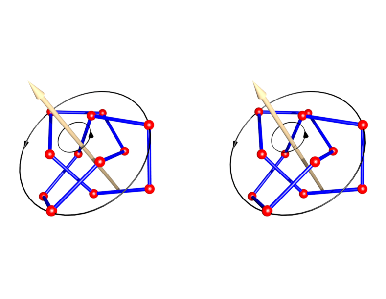
Figure 3: A 3D cross-eye view of the minimum energy time crystal solution with Hamiltonian that is a combination of Coulomb attraction and Pauli exclusion. The beige arrow is the axis of rotation and the black circles show the direction of rotation.

The two examples of $N=12$ molecular rings, with the topologies of an unknot and a trefoil knot, show a general relation between knottiness and the time crystal state that we have observed. The critical point sets $\{\mathbf{x}_{i,cr}\}$ of our Hamiltonian functions always pertain to a definite string conformation, with a definite knot topology. But the topology of a generic knot is in general different from that of the critical point set of the Hamiltonian. For this reason a knotted molecular ring often tends to be timecrystalline.

6 Rotation Without Angular Momentum

The time crystals that we have constructed are all rotating rigid bodies. Since rotation engages energy and for a time crystal that should be minimal, we need to understand the origin of the effective theory timecrystalline rotational motion: Why is a rotational motion consistent with minimal mechanical free energy a.k.a. Hamiltonian. For this we first explain how an apparent rigid rotation can arise in the absence of any angular momentum, in the case of a deformable body. We then propose that rotation without angular momentum can be viewed as the atomic level origin of the time crystals that we have constructed, in the framework of an effective theory Hamiltonian description.

It is well known that when a deformable body contains at least three independently movable components, its vibrational and rotational motions are no longer separable [16, 17, 18, 19, 20]. Small local vibrations of a deformable body can self-organize into a global, uniform rotation of the entire body. This is a phenomenon that is used widely for control purposes. For example, the position and altitude of satellites are often controlled by periodic motions of parts of the satellite, such as spinning rotors.

To describe how this kind of atomic level self-organization takes place, and how it can lead to an apparent timecrystalline dynamics at the level of an effective Hamiltonian theory, we consider the simplest possible example, that of a deformable triangle with three equal unit mass point particles at its vertices $\mathbf{r}_{i}(t)$ ($i=1,2,3$). We assume that no external forces act on the triangle so that the center of mass remains stationary,

$$\mathbf{r}_{1}+\mathbf{r}_{2}+\mathbf{r}_{3}=0$$

at all times. We also assume that there is no net rotation so that the total angular momentum $\mathbf{L}$ vanishes,

$$\mathbf{L}\ =\ \mathbf{r}_{1}\wedge\dot{\mathbf{r}}_{1}+\mathbf{r}_{2}\wedge\dot{\mathbf{r}}_{2}+\mathbf{r}_{3}\wedge\dot{\mathbf{r}}_{3}\ =\ 0$$ (37)

We can orient the triangle to always lay on the $z=0$ plane. We then allow the triangle to change its shape in an arbitrary fashion: Two triangles have the same shape when they differ from each other only by a rigid rotation, and we describe shape changes using shape coordinates $\mathbf{s}_{i}(t)$ with

$$\mathbf{s}_{1}+\mathbf{s}_{2}+\mathbf{s}_{3}=0$$

that we assign to the vertices. These coordinates describe unambiguously all possible triangular shapes when we demand that $s_{1x}>0$, $s_{1y}=0$ and $s_{2y}>0$.

At each time $t$ the shape coordinates $\mathbf{s}_{i}(t)$ relate to the space coordinates $\mathbf{r}_{i}(t)$ by a spatial rotation on the $z$-plane,

$$\mathbf{r}_{i}(t)\ =\ \mathcal{O}(t)\mathbf{s}_{i}(t)\ \ \ \ \ \ {\rm with}\ \ \ \ \ \ \mathcal{O}(t)\ =\ \left(\eqalign{\cos\theta(t)\ -\sin\theta(t)\\ \sin\theta(t)\ \ \ \ \cos\theta(t)}\right)$$ (38)

We consider a triangle that changes its shape in a periodic, but otherwise arbitrary fashion; the triangle traces a closed loop $\Gamma$ in the space of all possible triangular shapes. We assume that initially, at time $t=0$, the triangle is e.g. equilateral and that it returns back to its original shape at a later time $t=\mathrm{T}$. During the time period $\mathrm{T}$ it may have rotated in space, by an angle $\theta(\mathrm{T})$. To evaluate this angle we substitute (38) into (37). This gives us

$$\theta(\mathrm{T})\ =\ \int\limits_{0}^{\mathrm{T}}\!dt\,\,\frac{\sum\limits_{i=1}^{3}\left\{s_{iy}\dot{s}_{ix}-s_{ix}\dot{s}_{iy}\right\}}{\sum\limits_{i=1}^{3}\mathbf{s}^{2}_{i}}\ \equiv\ \int_{\Gamma}d{\mathbf{l}}\cdot{\mathbf{A}}$$ (39)

We identify here a connection one-form $\mathbf{A}$, it computes the rotation angle $\theta(\mathrm{T})$ as a line integral over the periodic, closed trajectory $\Gamma$ in the space of all possible triangular shapes [16, 17, 18, 19, 20]. To interpret $\mathbf{A}$ geometrically, we proceed as follows: We first represent the three coordinates $\mathbf{s}_{i}$ in terms of the Jacobi coordinates $\boldsymbol{\rho}_{1},\ \boldsymbol{\rho}_{2}$ of the classical three-body problem,

$$\cases{\mathbf{s}_{1}=\frac{1}{\sqrt{2}}\boldsymbol{\rho}_{1}-\frac{1}{\sqrt{6}}\boldsymbol{\rho}_{2}\\ \mathbf{s}_{2}=\sqrt{\frac{2}{3}}\boldsymbol{\rho}_{2}\\ \mathbf{s}_{3}=-\frac{1}{\sqrt{2}}\boldsymbol{\rho}_{1}-\frac{1}{\sqrt{6}}\boldsymbol{\rho}_{2}}\ \ \ \ \ \ s\in[0,2\pi)$$ (40)

We denote

$$\boldsymbol{\rho}_{1}=r\cos\frac{\vartheta}{2}\left(\eqalign{\cos\phi_{1}\\ \sin\phi_{1}}\right)\ \ \ \ \&\ \ \ \ \boldsymbol{\rho}_{2}=r\sin\frac{\vartheta}{2}\left(\eqalign{\cos\phi_{2}\\ \sin\phi_{2}}\right)$$

We define $\phi_{\pm}=\phi_{1}\pm\phi_{2}$ and we combine the coordinates into standard spherical coordinates,

$$\eqalign{x=r\sin\vartheta\cos\phi_{-}\\ y=r\sin\vartheta\sin\phi_{-}\\ z=r\cos\vartheta}$$

The connection one-form $\mathbf{A}$ is then

$$\mathbf{A}\ =\ -\frac{1}{2}\cos\vartheta d\phi_{-}-\frac{1}{2}d\phi_{+}\ =\ \frac{1}{2}\frac{\ xdy-ydx}{r(r+z)}\ -\ \frac{1}{2}(d\phi_{+}+d\phi_{-})$$ (41)

where recognize the connection one-form of a single Dirac magnetic monopole in $\mathbb{R}^{3}$, located at the origin $r=0$ and with its string placed along the negative $z$-axis; see also [24]. Thus the rotation angle $\theta(\mathrm{T})$ in (39) computes the (magnetic) flux of the Dirac monopole through a surface with boundary $\Gamma$, in the space of all triangular shapes. We note that at the location of the monopole all three vertices of the triangle overlap, and the string corresponds to a shape where two of the vertices overlap.

We proceed to evaluate the rotation angle (39) in the case of the following (quasi)periodic family of triangles,

$$\mathbf{s}_{1}(t)\ =\ \frac{1}{\sqrt{3}}\left(\eqalign{\cos(f[t])\\ \hskip 17.07182pt0}\right)\ \ \ \ \ \ \&\ \ \ \ \ \ \mathbf{s}_{2}(t)\ =\ \frac{1}{\sqrt{3}}\left(\eqalign{\cos(g[t]+\frac{2\pi}{3})\\ \hskip 17.07182pt\sin(\frac{2\pi}{3})}\right)$$ (42)

where we recall that $\mathbf{s}_{3}(t)=-\mathbf{s}_{1}(t)-\mathbf{s}_{2}(t)$ and

$$f(t)=f(t+n\mathrm{T}_{1})\ \ \ \ \ {\rm with}\ \ \ \ \ f(0)=0$$

and

$$g(t)=g(t+n\mathrm{T}_{2})\ \ \ \ \ {\rm with}\ \ \ \ \ g(0)=0$$

so that initially at $t=0$ we indeed have an equilateral triangle, with unit length edges. We choose

$$f[t]=a\sin\omega_{1}t\ \ \ \ \&\ \ \ \ \ g_{1}[t]=a\sin\omega_{2}t$$ (43)

with amplitude $|a|<1$ and positive frequencies $\omega_{1,2}$.

The shape changes (42), (43) can be interpreted e.g. as (small amplitude) oscillations of atoms that are located at the vertices of a triangular molecule. We do not specify the mechanism that gives rise to (43); the origin of these oscillations could be e.g. quantum mechanical. We are only interested in an effective theory description, that becomes valid in the limit of time scales that are very large in comparison to the periods of the small, rapid vibrational motions.

For generic $\omega_{1}$ and $\omega_{2}$ the integrand of (39) is quasiperiodic, thus by Riemann’s lemma we expect that for generic $\omega_{1,2}$ the large time limit of $\theta(t)$ vanishes so that there is no net rotational motion. However, it turns out that exactly for $\omega_{2}=\pm 2\omega_{1}$ the large time limit describes a uniformly rotating triangle. To see how this comes about we expand the integrand of (39) in powers of (small) $a$,

$$\frac{d\theta}{dt}\ =\ -\frac{1}{2}\omega_{2}a\cos\omega_{2}t+\frac{\sqrt{3}}{12}a^{2}\left\{\omega_{2}\sin 2\omega_{2}t-\omega_{1}\sin 2\omega_{1}t\right\}-\frac{1}{8}\omega_{2}a^{3}\cos 3\omega_{2}t$$

$$+\frac{1}{16}\omega_{2}a^{3}\left\{\cos(\omega_{2}+2\omega_{1})t+\cos(\omega_{2}-2\omega_{1})t\right\}+{\mathcal{O}}(a^{4})$$ (44)

Thus, exactly when $\omega_{2}=\pm 2\omega_{1}$ the large time limit of the rotation angle $\theta(t)$ increases linearly in time as follows,

$$\theta(t)\ \buildrel{{\rm large}-t}\over{\longrightarrow}\ \frac{1}{16}\,\omega_{2}a^{3}t$$ (45)

In Figures 4 a)-d) we summarize the time evolution of $\theta(t)$ when we observe its value stroboscopically, like frames of a movie reel, at regular fixed time steps $\Delta t(n)=10^{n}$ for $n=0,1,2,4$.

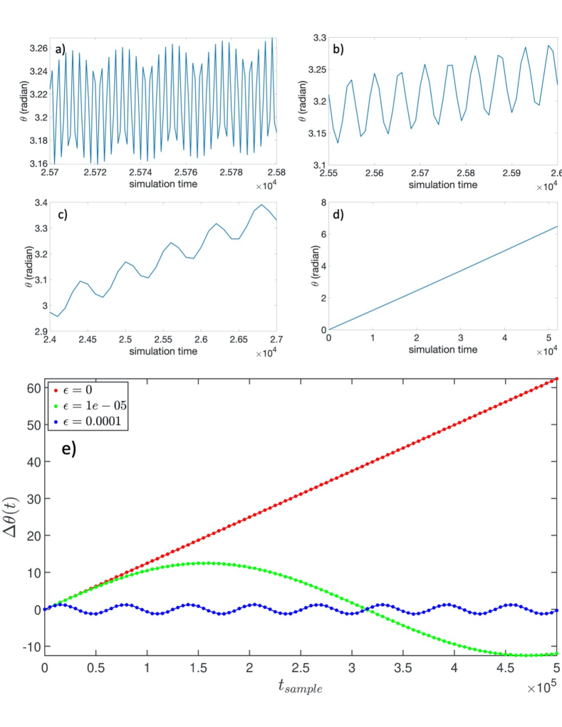
Figure 4: Figure a) shows the time evolution of rotation angle $\theta(t)$ in (39) when we sample it with stroboscopic time step $\Delta t=1$. In Figure b) the time step is increased to $\Delta t=10$, in Figure c) $\Delta t=100$ and in Figure d) $\Delta t=10.000$. In all these Figures $\omega_{2}=2\omega_{1}=2$ and $a=0.1$. Figure e) then shows the transition from uniform rotation at $\omega_{2}=2\omega_{1}=2$ to a sisyphus-like ratcheting motion for $\omega_{2}=2\omega_{1}+\epsilon$ with $\epsilon=10^{-5}$ and $\epsilon=10^{-4}$. For each trajectory in Figure e) $\omega_{1}=1$, $a=0.2$ and $\Delta t=10.000$.

$\bullet~{}$ The Figure 4 a) shows that when we sample the values of $\theta(t)$ with stroboscopic time step $\Delta t=1$, the dominant motion consists of rapid and slightly irregular back and forth oscillations; the irregularities are due to higher order harmonics that are not properly caught by the stroboscope. On top of the rapid oscillations we observe lower frequency undulations, five periods are shown in the Figure.

We also observe a very slow increase in the time averaged value of $\theta(t)$. This indicates the potential presence of a slow clockwise drifting rotation of the triangle around an axis that is normal to its plane.

$\bullet~{}$ In Figure 4 b) we increase the stroboscopic time step to $\Delta t=10$. We observe slightly irregular back and forth oscillations with an essentially constant amplitude, with a wavelength that is clearly larger than those in Figure 4 a). In addition, there is a much more visible increase in the average value of $\theta(t)$. It describes a clockwise rotational ratcheting of the triangle around its normal axis.

$\bullet~{}$ When the time step increases to $\Delta t=100$, as shown in Figure 4 c) the triangle continues to ratchet in the clockwise direction around its normal axis. The relative amplitude of the slightly irregular back and forth oscillations has diminished, while the wavelength has increased. The same qualitative behaviour persists when we increase $\Delta t=1000$, but with increasingly diminished amplitude and increased wavelength.

$\bullet~{}$ When we increase the stroboscopic time step to the much larger value $\Delta t=10000$ the motion closely resembles that of an equilateral triangle that rotates uniformly around its symmetry axis in clockwise direction, with constant angular velocity that can be estimated from (45). See Figure 4 d).

$\bullet~{}$ In Figure 4 e) we show how the uniform, large stroboscopic time scale rotation that we observe for $\omega_{2}=2\omega_{1}$ and display in Figure 4 d) converts into back and forth rotations with an amplitude that eventually fades away, when $\epsilon=\omega_{2}-2\omega_{1}$ increases.

From the Figures we deduce that beyond the back and forth oscillations that dominate at the very short stroboscopic time scale as shown in Figure 4 a), there is a transitory regime shown in Figures 4 b) and c). In this regime the various high frequency oscillations self-organize into a ratcheting rotation of the triangle. The motion resembles the ”Sisyphus dynamics” described in [2, 25]. Accordingly we designate this regime as a pre-timecrystalline sisyphus stage. We expect that in this regime the motion of the triangle can be modeled by a version of the “Sisyphus Lagrangian” [25].

Finally, in the limit of very large stroboscopic time scale shown in Figure 4 d) the ratcheting motion fades away. In this limit, where we inspect the triangle at time scales that are much larger than the characteristic timescale of the shape changes e.g. $T_{1}\sim 2\pi/\omega_{1}$, we can only observe a uniform rotation. In particular, in this large time scale limit the triangle rotates exactly in the same manner as the time crystalline triangle with Hamiltonian (32) and Poisson bracket (18) rotates, as shown in Figure 1 b).

Thus, we can interpret the Hamiltonian time crystal (18), (32) as an effective theory description of the deforming $\omega_{2}=\pm\omega_{1}$ triangle, in the large time scale limit.

7 Summary

We have identified a Hamiltonian time crystal as a time dependent minimum energy symmetry transformation, that spontaneously breaks a continuous symmetry group into an abelian subgroup. For such a timecrystalline spontaneous symmetry breaking to occur, the Hamiltonian dynamics needs to take place on a presymplectic phase space.

As an example we have analyzed a general family of Hamiltonian models, designed to describe the dynamics of piecewise linear polygonal closed strings. The vertices of the string are pointlike interaction centers, they are connected to each other by links that are free to move in any possible way except for stretching, shrinking and chain crossing.

The family of string Hamiltonians that we have analyzed, are commonly encountered in coarse grain descriptions of stringlike atoms and small molecules. We have argued that the ensuing timecrystalline Hamiltonian dynamics is an effective theory description that becomes valid in a large time scale limit, when the very rapid individual atomic level vibrations can be ignored and replaced by much slower collective oscillations.

Finally, in the case of a triangular structure, we have found that the effective timecrystalline Hamiltonian dynamics reflects the presence of a Dirac monopole in a presymplectic phase space that describes all possible triangular shapes.

Our results propose that physical realizations of time crystals could be found in terms of knotted ring molecules.

References

References

- [1] F. Wilczek, Phys. Rev. Lett. 109 160401 (2012)
- [2] A. Shapere, F. Wilczek, Phys. Rev. Lett. 109 160402 (2012)
- [3] F. Wilczek, Phys. Rev. Lett. 111 250402 (2013)
- [4] K. Sacha, J. Zakrzewski, Rep. Prog. Phys. 81 016401 (2018)
- [5] P. Bruno, Phys. Rev. Lett. 110 118901 (2013)
- [6] H. Watanabe, M. Oshikawa, Phys. Rev. Lett. 114 251603 (2014)
- [7] J. Dai, A.J. Niemi, X. Peng, F. Wilczek, Phys. Rev. A99 023425 (2019)
- [8] J. Dai, X. Peng, A.J. Niemi, arXiv preprint arXiv:1910.13787
- [9] A. Alekseev, J. Dai, A.J. Niemi, arXiv preprint arXiv:2002.07023
- [10] A. Wasserman, Topology 8 127 (1969)
- [11] A.J. Niemi, K. Palo, arXiv:hep-th/9406068
- [12] D.M. Austin and P.J. Braam, Morse-Bott theory and equivariant cohomology (The Floer memorial volume, 123-183, Progr. Math., 133, Birkh user, Basel, 1995)
- [13] L. Nicolaescu, An Invitation to Morse Theory (Second Edition, Springer Verlag, New York, 2011)
- [14] J.E. Marsden and T.S. Ratiu, Introduction to Mechanics and Symmetry A Basic Exposition of Classical Mechanical Systems Second Edition (Springer Verlag, New York, 1999)
- [15] A.R. Leach, Molecular Modelling: Principles and Applications (Prentice Hall, Upper Saddle River, 2001)
- [16] A. Guichardet, Annales de l’Institut Henri Poincaré 40 329(1984)
- [17] A. Shapere, F. Wilczek, Am. J. Phys. 57, 514(1989)
- [18] A. Shapere, F. Wilczek, Journ. Fluid Mech. 198 557(1989)
- [19] R.G. Littlejohn, M. Reinsch, Rev. Mod. Phys. 69 213 (1997)
- [20] J.E. Marsden, Geometric foundations of motion and control, in Motion, Control, and Geometry: Proceedings of a Symposium (National Academy Press, Washington, 1997)
- [21] J.H. Conway, H. Burgiel, C. Goodman-Strauss The symmetries of things (A. K. Peters, Wellesley, 2008)
- [22] W. Gibb, Math. Sch. 19 2(1990)
- [23] O. Kratky, G. Porod, Rec. Trav. Chim. 68 1108 (1949)
- [24] F. Wilczek, arXiv:1912.08092
- [25] A. Shapere, F. Wilczek, PNAS 116 18772 (2019)