Improving Robustness via Risk Averse Distributional Reinforcement Learning

Abstract

One major obstacle that precludes the success of reinforcement learning in real-world applications is the lack of robustness, either to model uncertainties or external disturbances, of the trained policies. Robustness is critical when the policies are trained in simulations instead of real world environment. In this work, we propose a risk-aware algorithm to learn robust policies in order to bridge the gap between simulation training and real-world implementation. Our algorithm is based on recently discovered distributional RL framework. We incorporate CVaR risk measure in sample based distributional policy gradients (SDPG) for learning risk-averse policies to achieve robustness against a range of system disturbances. We validate the robustness of risk-aware SDPG on multiple environments.

1 Introduction

Reinforcement learning (RL) has been successful in achieving human level or even better performance (Mnih et al., 2015a; Silver et al., 2017) in multiple games such as Atari and Go. However, one of the major factors hindering the application of RL to real-world continuous control tasks is the modeling gap between simulation and real-world which can lead to unpredictable, and often unwanted, results (Pinto et al., 2017). More specifically, learning policies requires a large amount of training data, which is expensive to collect if trained directly in real-world environment. Thus, simulators are often used for learning policies before deploying to real-world problems. However, such simulation models usually contain uncertainties, i.e., a reality gap, which makes the policies trained in simulation less desirable in real applications. In this paper, we propose an algorithm to improve the robustness of RL against such model uncertainties.

There are two popular approaches to robust RL: by minimizing the expected loss in the worst case via minimax formulations (Heger, 1994; Nilim and El Ghaoui, 2005; Tamar et al., 2014; Pinto et al., 2017) and by considering risk-sensitive optimization criteria during training (Chow and Ghavamzadeh, 2014; Tamar et al., 2015). The relation between the two has been studied in Jacobson (1973); Coraluppi and Marcus (1999); Glover and Doyle (1988); Fleming and McEneaney (1992, 1995). Our proposed algorithm falls into the latter. In particular, we incorperate risk-sensitive criteria within distributional reinforcement learning (DRL) framework. Instead of modeling the value function as the expected sum of rewards, the DRL (Bellemare et al., 2017) framework suggests to work with the full distribution of random returns, known as value or return distribution, i.e., $Q^{\pi}(x,a)={\mathbb{E}}Z^{\pi}(x,a)$, where $Z^{\pi}(x,a)$ denotes the return distribution. The return distribution $Z$ in DRL framework provides tremendous flexibility to incorporate risk in the training process.

In DRL, the return distribution is usually represented by discrete categorical form (Bellemare et al., 2017; Barth-Maron et al., 2018; Qu et al., 2018), quantile function (Dabney et al., 2018b; Zhang et al., 2019), or samples (Freirich et al., 2019; Singh et al., 2020). D4PG (Barth-Maron et al., 2018) and SDPG (Singh et al., 2020) are actor-critic type policy gradient algorithms based on DRL and have demonstrated much better performance (Barth-Maron et al., 2018; Tassa et al., 2018) as compared to its non-distributional counterpart (DDPG) (Silver et al., 2014) for continuous control tasks. In SDPG, the return distribution is represented via samples as opposed to discrete categorical representation in D4PG, which has shown advantages in terms of sample efficiency as well as maximum rewards. Even though D4PG and SDPG learn the return distribution, they optimize the mean value of the returns and therefore, are susceptible to model uncertainties. In this work, we incorporate risk-sensitive criteria for optimizing the policy in SDPG algorithm to achieve robustness against a range of disturbances in the system. Specifically, we focus on conditional value at risk (CVaR) (Chow and Ghavamzadeh, 2014; Chow et al., 2015), a widely adopted risk measure.

We perform multiple experiments to illustrate the robustness of the learned policy incorporating the risk during training against the risk-neutral policy. We demonstrate the robustness of our risk-averse SDPG algorithm against system disturbances on multiple OpenAI Gym (Brockman et al., 2016) environments for continuous control tasks including BipedalWalker, HalfCheetah, and Walker2d.

Related Work: There have been a few methods which accounted for risk within DRL framework including Morimura et al. (2010a, b); Dabney et al. (2018a); Tang et al. (2019). The distributional-SARSA-with-CVaR proposed in  Morimura et al. (2010a, b) deals with discrete action space with only a small number of states. Although implicit quantile network (IQN) proposed in Dabney et al. (2018a) improved upon traditional deep Q-networks (DQNs) (Mnih et al., 2015b) and studied risk-sensitive policies in Atari games, it is a value function based approach and thus not suitable for tasks with continuous action space. Worst cases policy gradients (WCPG) proposed in Tang et al. (2019) models the return distribution $Z$ as Gaussian in order to calculate CVaR in closed form, but this restriction may undermine the advantages of DRL. In terms of taxonomy presented by Garcıa and Fernández (2015), our approach lies in the risk-sensitive criterion.

The contributions of this work are as follows: (a) We propose a novel RL algorithm to learn robust policies for continuous control tasks. Our algorithm is based on the recently discovered DRL framework. The fact that DRL learns the distribution instead of the mean of the cost-to-go function makes it suitable for risk-sensitive learning. We further took advantage our recent algorithm SDPG (Singh et al., 2020) to evaluate the risk criteria efficiently using samples. (b) We empirically evaluate the performance of our algorithm on multiple OpenAI Gym environments.

Rest of the document is organized as follows. First we briefly discuss background on DRL, SDPG, and risk measures in Section 2. Next, we present our risk-averse SDPG algorithm in Section 3 followed by experimental results in Section 4. Finally, Section 5 concludes the paper.

2 Background

We consider standard RL setting where the interaction of an agent with an environment is modeled as $({\mathcal{X}},{\mathcal{A}},R,P,\gamma)$. Here, ${\mathcal{X}},{\mathcal{A}}$ denote the state and action spaces respectively, $P(\cdot\mid x,a)$ is the transition kernel, $\gamma\in[0,1]$ is the discount factor, and $R(x,a)$ is the reward of taking action $a$ at state $x$. Our focus in this paper is on continuous state and action spaces and deterministic policies $a_{t}=\pi(x_{t})$. Traditional RL aims to find a stationary policy $\pi$ that maximizes the Q-function which is the expected long-term discounted reward

$$Q^{\pi}(x,a)={\mathbb{E}}\left[\sum_{t=0}^{\infty}\gamma^{t}R(x_{t},a_{t})\right],~{}~{}x_{t}\sim P(\cdot\mid x_{t-1},a_{t-1}),a_{t}=\pi(x_{t}),x_{0}=x,a_{0}=a.$$ (1)

The Q-function is characterized by Bellman’s equation (Bellman, 1966)

$$Q^{\pi}(x,a)={\mathbb{E}}R(x,a)+\gamma{\mathbb{E}}Q^{\pi}(x^{\prime},\pi(x^{\prime})\mid x,a).$$ (2)

2.1 DRL

Distributional reinforcement learning (DRL) models intrinsic randomness of return in form of full return distribution for each state-action pair

$$Z^{\pi}(x,a)=\sum_{t=0}^{\infty}\gamma^{t}R(x_{t},a_{t}),~{}~{}x_{t}\sim P(\cdot\mid x_{t-1},a_{t-1}),a_{t}=\pi(x_{t}),x_{0}=x,a_{0}=a.$$ (3)

Apparently, Q-function is the mean of return distribution, i.e., $Q^{\pi}(x,a)={\mathbb{E}}Z^{\pi}(x,a)$. The return distribution satisfies distributional Bellman’s equation (Bellemare et al., 2017)

$$Z^{\pi}(x,a)=R(x,a)+\gamma Z^{\pi}(x^{\prime},\pi(x^{\prime})\mid x,a),$$ (4)

where the equality is in the probability sense.

Different methods have been proposed to parameterize a return distribution in DRL. C51 (Bellemare et al., 2017) and D4PG (Barth-Maron et al., 2018) use discrete categorical distribution, QR-DQN (Dabney et al., 2018b) and IQN (Dabney et al., 2018a) utilize quantiles, and VDGL (Freirich et al., 2019) and SDPG (Singh et al., 2020) use samples to model a return distribution. These DRL algorithms have shown significant performance improvements over non-distributional counterparts in multiple environments including Atari games and DeepMind Control Suite (Tassa et al., 2018).

2.2 SDPG

Sample based policy gradient (SDPG) (Singh et al., 2020) is an actor-critic type policy gradient method within DRL framework where return distribution is represented by samples through a reparametrization technique (Kingma and Welling, 2013). The actor network in SDPG parameterizes the policy while the critic network is trained to mimic the return distribution determined via distributional Bellman equation based on samples. A flow diagram of the critic in SDPG is shown in Figure 1. The critic network $G_{\phi}$ in SDPG learns the return distribution by utilizing quantile Huber loss (Huber, 1964; Dabney et al., 2018b) as a surrogate of Wasserstein distance:

$$L_{critic}(\phi)=\mathbb{E}\left[\frac{1}{n^{2}}\sum_{i=1}^{n}\sum_{j=1}^{n}\rho_{\hat{\tau}_{i}}^{\zeta}(\tilde{z}_{j}-z_{i})\right],$$ (5)

where $z_{1}\geq z_{2}\geq\ldots z_{n}$ are samples after sorting. Moreover, $\rho^{\zeta}_{\hat{\tau}_{i}}(v)=|\hat{\tau}_{i}-\delta_{\{v<0\}}|L_{\zeta}(v)$,

$$L_{\zeta}(v)=\begin{cases}0.5\,v^{2}&\text{if~{}}|v|<\zeta\\ \zeta(|v|-0.5~{}\zeta)&\text{otherwise,}\end{cases}$$

and $\hat{\tau}_{i}=\frac{1}{2}(\tau_{i}+\tau_{i-1}),~{}~{}i=1,2,\ldots,n$ with $\tau_{i}=\frac{i}{n}$.

Using the distributional policy gradient theorem (Barth-Maron et al., 2018), the gradient of the loss function of the actor network $\pi_{\theta}$ is computed as

$$\nabla_{\theta}L_{actor}(\theta)\!\!=\!\!\mathbb{E}\left[\nabla_{\theta}\pi_{\theta}(x)~{}\frac{1}{n}\sum_{j=1}^{n}\left[\nabla_{a}z_{j}\right]|_{a=\pi_{\theta}(x)}\right].$$ (6)

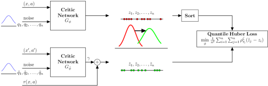
Figure 1: Flow diagram of SDPG.

2.3 Risk Measures

The notion of risk in RL is related to the fact that even an optimal policy may perform poorly in some cases due to the stochastic nature of the problem. Risk-aware methods in RL have considered different forms of risk (L.A. and Fu, 2018) including the variance of the return, worst outcomes, exponential utility function, value at risk (VaR), and conditional value at risk (CVaR) (Chow and Ghavamzadeh, 2014). In this work, we focus on CVaR.

CVaR of a random variable $Z$ at level $\alpha\in[0,1]$ is defined as

$$\text{CVaR}_{\alpha}(Z):=\mathbb{E}~{}[Z~{}|~{}Z\leq\text{VaR}_{\alpha}(Z)]$$ (7)

Let $\{z_{i}\}_{i=1}^{n}$ be the i.i.d. samples from the distribution of $Z$ and let $\{z_{[i]}\}_{i=1}^{n}$ be its order statistics with $z_{[1]}\leq z_{[2]}\leq\ldots\leq z_{[n]}$. Then CVaR at level $\alpha$ can be estimated as (Kolla et al., 2019)

$$\hat{c}_{n,\alpha}=\frac{1}{n(1-\alpha)}\sum_{i=1}^{n}z_{i}~{}\mathbb{I}\{z_{i}\leq\hat{v}_{n,\alpha}\},$$ (8)

where $\mathbb{I}\{.\}$ is the indicator function, and $\hat{v}_{n,\alpha}$ is estimated VaR from samples $\hat{v}_{n,\alpha}=z_{[\lfloor n(1-\alpha)\rfloor]}$ with $\lfloor.\rfloor$ being floor function. When $\alpha=0$, CVaR becomes expectation of the random variable which reduces to risk-neutral setting.

3 Risk averse SDPG

In order to take risk into account in policy learning, we utilize the return distribution to incorporate risk. We use CVaR as the risk-measure to learn the policy. Similar to SDPG, the risk-sensitive SDPG consists of two neural networks: a critic and an actor. The critic network $G_{\phi}$, parameterized by $\phi$, generates samples representing the return distribution by reparameterizing noise for each state-action pair. These samples are compared against the target samples determined via distributional Bellman equation given by (4). The quantile Huber loss is used for updating the critic network as given by Equation (5).

Algorithm 1 Risk-averse SDPG

  Require: Learning rates $\beta_{1}$ and $\beta_{2}$, CVaR level $\alpha$, batch size $M$, sample size $n$, exploration constant $\delta$,

  Initialize the the actor network ($\pi$) parameters $\theta$, critic network ($G$) parameters $\phi$ randomly

  Initialize target networks $(\tilde{\theta},\tilde{\phi})\leftarrow(\theta,\phi)$

  for the number of environment steps do

     Sample $M$ number of transitions $\{(x_{t}^{i},a_{t}^{i},r_{t}^{i},x_{t+1}^{i})\}_{i=1}^{M}$ from the replay pool

     Sample noise $\{q_{j}^{i}\}_{j=1}^{n}\sim\mathcal{N}(0,1)$ and $\{\tilde{q_{j}}^{i}\}_{j=1}^{n}\sim\mathcal{N}(0,1)$,  for  $i=1,\ldots,M$

     Apply Bellman update to create samples (of return distribution)

$$\tilde{z}_{j}^{i}=r_{t}^{i}+\gamma G_{\tilde{\phi}}(\tilde{q_{j}}^{i}|(x_{t+1}^{i},\pi_{\tilde{\theta}}(x_{t+1}^{i})))\quad\mathrm{for}~{}j=1,2,\ldots,n$$

     Generate samples $z_{j}^{i}=G_{\phi}(q_{j}^{i}|(x_{t}^{i},a_{t}^{i}))\quad\mathrm{for}~{}j=1,2,\ldots,n$

     Sort the samples $z^{i}$ in ascending order

     Update $G_{\phi}$ by stochastic gradient descent with learning rate $\beta_{1}$:

$$\frac{1}{M}\sum_{i=1}^{M}\frac{1}{n^{2}}\sum_{j=1}^{n}\sum_{k=1}^{n}\rho_{\hat{\tau}_{j}}^{\zeta}(\tilde{z}_{k}^{i}-z_{j}^{i})$$

     Update $\pi_{\theta}$ by stochastic gradient ascent with learning rate $\beta_{2}$:

$$\frac{1}{M}\sum_{i=1}^{M}\pi_{\theta}(x_{t}^{i})~{}\nabla_{a}\left[\frac{1}{n(1-\alpha)}\sum_{j=1}^{n}z_{j}^{i}~{}\mathbb{I}\{z_{j}^{i}\leq z_{\lfloor n(1-\alpha)\rfloor}^{i}\}\right]_{a=\pi_{\theta}(x_{t}^{i})}$$

     Update target networks $(\tilde{\theta},\tilde{\phi})\leftarrow(\theta,\phi)$

  end for

  Actor

  repeat

     Observe $(x_{t},a_{t},x_{t+1})$ and draw reward $r_{t}$

     Sample action $a_{t+1}=\pi_{\theta}(x_{t+1})+\delta\mathcal{N}(0,1)$

     Store $(x_{t},a_{t},r_{t},x_{t+1},a_{t+1})$ in replay pool

  until learner finishes

The actor network $\pi_{\theta}$, parameterized by $\theta$, outputs the action $\pi_{\theta}(x)$ given a state $x$. The actor network incorporates risk as feedback from the critic network $G_{\phi}$ in terms of the gradients of the empirical CVaR (given by Equation 8) of the return distribution with respect to the actions determined by the policy. This feedback is used to update the actor network by applying distributional form of the policy gradient theorem. Therefore, the gradient of the actor network loss function is

$$\nabla_{\theta}L_{actor}(\theta)\!\!=\!\!\mathbb{E}\left[\nabla_{\theta}\pi_{\theta}(x)~{}\nabla_{a}\left[\frac{1}{n(1-\alpha)}\sum_{j=1}^{n}z_{j}~{}\mathbb{I}\{z_{j}\leq\hat{v}_{n,\alpha}\}\right]_{a=\pi_{\theta}(x)}\right],$$ (9)

where $\hat{v}_{n,\alpha}=z_{\lfloor n(1-\alpha)\rfloor}$.

All the steps of risk-averse SDPG algorithm are described in Algorithm 1. The network parameters of actor and critic networks are updated alternatively in stochastic gradient ascent/descent fashion.

4 Experiments

We evaluate the robustness of our risk-averse SDPG algorithm against system disturbances on multiple OpenAI Gym (Brockman et al., 2016) continuous control tasks. For both actor and critic networks, we use a two layer feedforward neural network with hidden layer sizes of 400 and 300, respectively, and rectified linear units (ReLU) between each hidden layer. We also used batch normalization on all the layers of both networks. Moreover, the output of the actor network is passed through a hyperbolic tangent (Tanh) activation unit. In all experiments we use learning rates of $\beta_{1}=\beta_{2}=1\times 10^{-4}$, batch size $M=256$, exploration constant $\delta=0.3$, and $\zeta=1$. Across all the tasks, we use $n=51$ number of samples to represent return distributions. Moreover, we run each task for a maximum of 1000 steps per episode. We consider four different levels of disturbances on action forces to evaluate the robustness of learned policies at different $\alpha$ levels of CVaR. We parameterize the disturbances in terms of Gaussian noise added to action forces during evaluation. We consider the disturbances at multiple noise scales to illustrate the robustness. For each environment, we consider different $NoiseLevel$ of the disturbances depending on the highest action value corresponding to the domain. Specifically, $NoiseLevel=0.3\times a_{max}$ is the variance of the added zero mean Gaussian noise with $a_{max}$ being the highest possible action value corresponding to the environment. Due to the lack of a perfect actuator, the experiments model scenarios when we deploy the policy to the real-world.

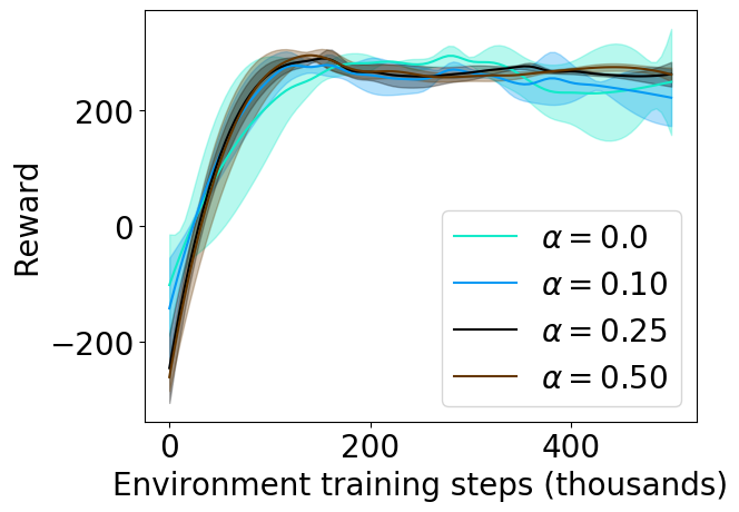
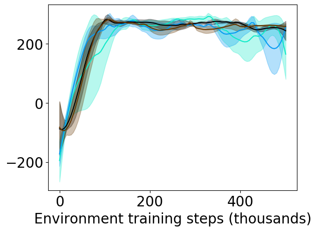
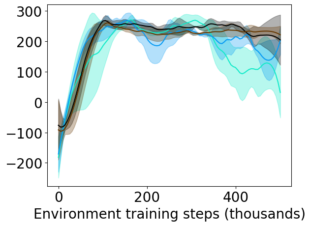
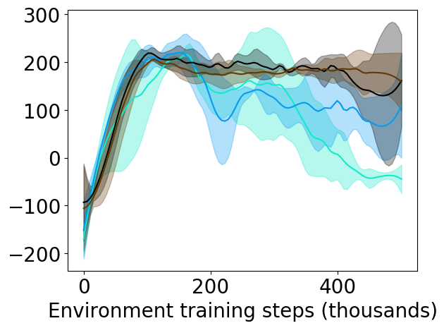
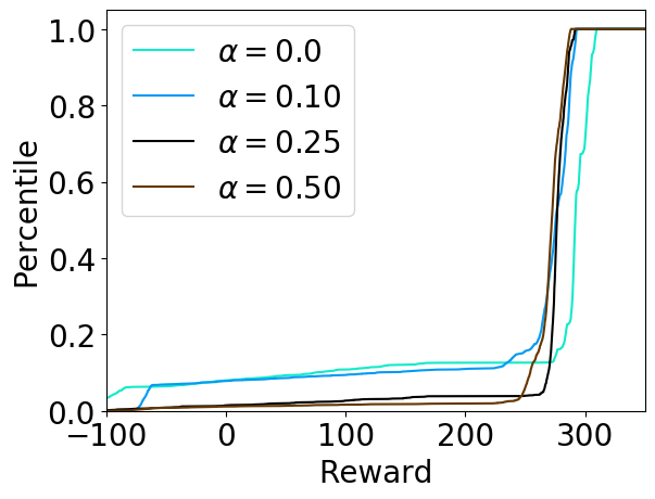
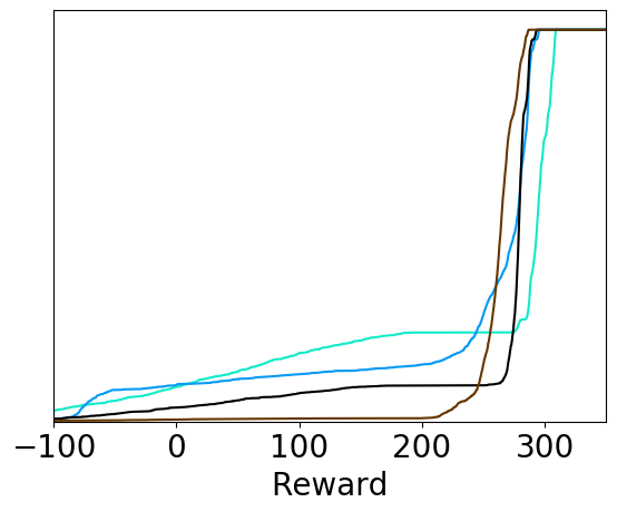
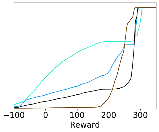
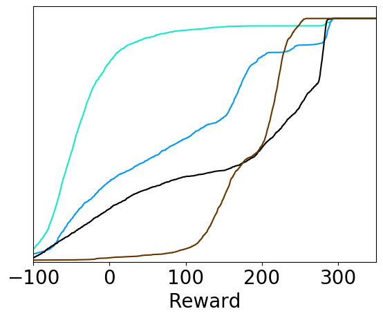
Figure 2: BipedalWalker-v2. Top row depicts evaluation curves and the bottom row depicts the CDFs at different noise levels. The evaluations are done every 5000 environment steps in each trial over 1000 episodes. The shaded region represents standard deviation of the average returns over 5 random seeds. The first column is noise-free, $NoiseLevel=0$. The second column is corresponding to $NoiseLevel=0.5$. The third one is $NoiseLevel=1.0$. The final column is $NoiseLevel=1.5$.

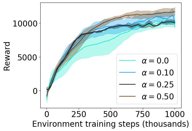
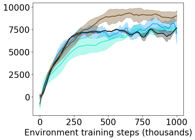
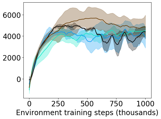
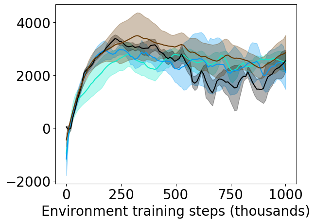
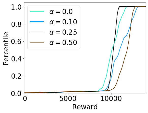
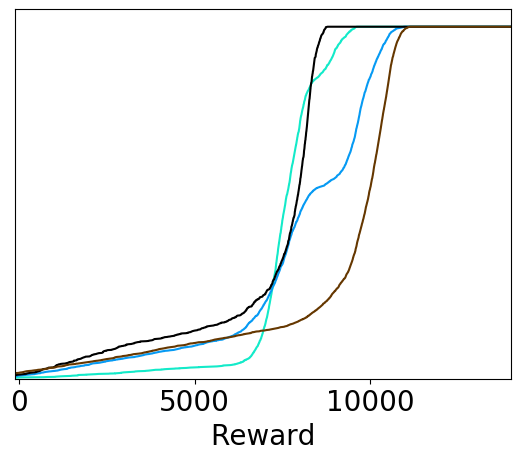
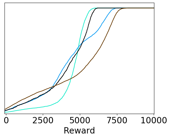
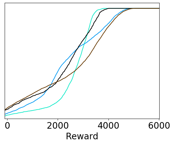
Figure 3: HalfCheetah-v2

We consider the following environments in our experiments: BipedalWalker-v2, HalfCheetah-v2, and Walker2d-v2. The task of an agent in all the three domains is to walk (run) as fast as possible without falling down and the reward is given for moving forward. We choose these environments because the reward has a large penalty when the robot falls down. These environments are not safe as compared to the other environments; the risky environment will have a value distribution with higher variance, which means there will be a higher probability that worst case scenario happens regardless of the expected reward. The state in BipedalWalker-v2 domain is 24-dimensional representing hull angle speed, angular velocity, horizontal speed, vertical speed, position of joints and joints angular speed, legs contact with ground, and $10$ lidar rangefinder measurements. The action space consists of actuator motor torques at 4 different joints. For both HalfCheetah-v2 and Walker2d-v2 domains, the state space is 18 dimensional consisting of positions, angles, and velocities of different joints while the dimension of action space is 6 consisting of actuator torques.

In each environment, we learn policies at different CVaR values $\alpha$ and evaluate the learned policies over 1000 trajectories for multiple levels of action disturbances. We also present the estimates of cumulative distribution functions (CDFs) from a total of 5000 rewards of trajectories. For all experiments in various environments, our risk-averse algorithms show similar performance during training compared to risk-neutral one.

Figure 2 shows the performance of our algorithm on BipedalWalker-v2 domain. The top row shows the evaluation curves at different noise levels and the bottom row depicts the corresponding CDFs. It can be observed from the figure that as noise level increases, the performance of all algorithms go down as expected. Moreover, our learned policies with non-zero CVaR $\alpha$ values outperform the risk-neutral one at all the noise levels. Figure 3 shows the performance in HalfCheetah-v2 environment. The policy with CVaR value 0.1 show the best performance at all the noise levels. Figure 4 shows the evaluation of our algorithm in Walker2d-v2 environment. The risk-neutral one is the most sensitive to the presence of noise. Risk-averse policy with CVaR value 0.5 show the most robustness in either noise free or noise environments.

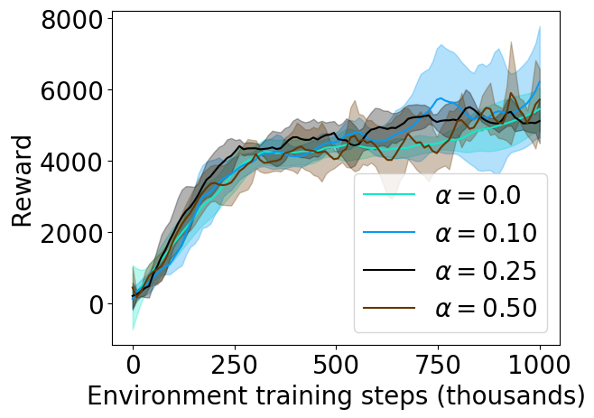
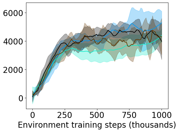
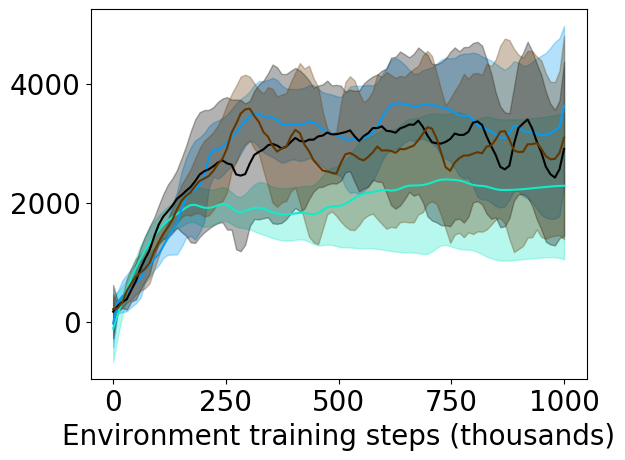
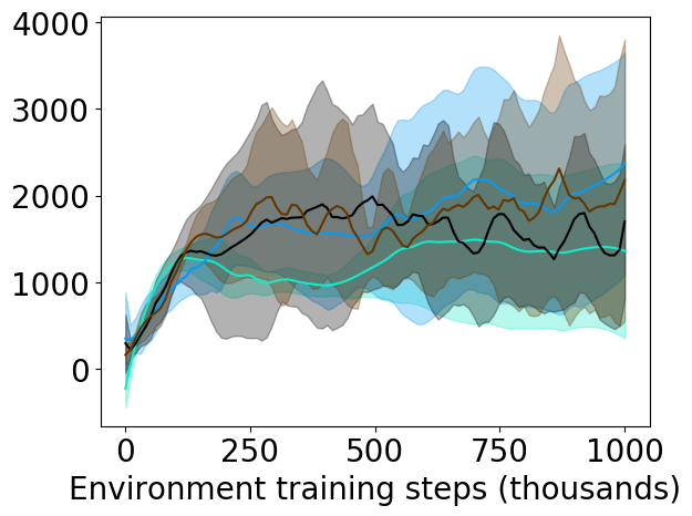
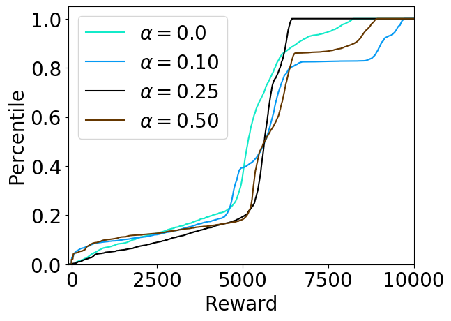
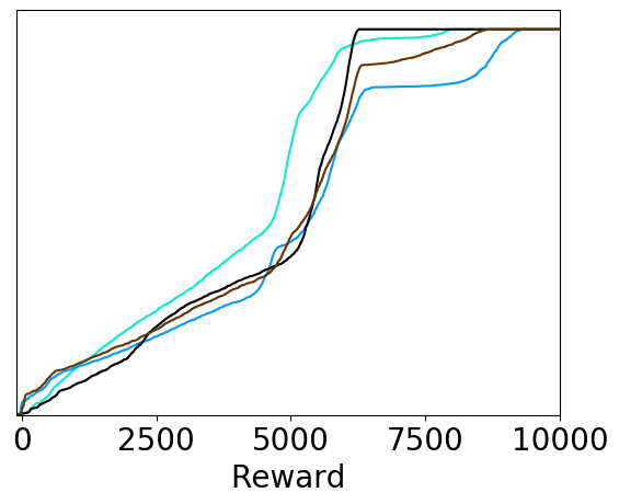
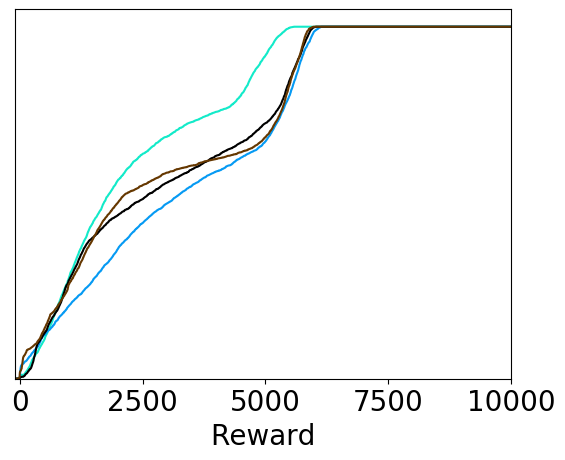
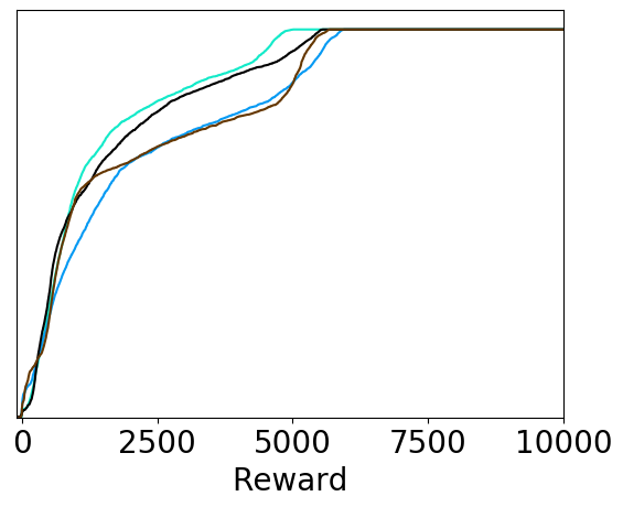
Figure 4: Walker2d-v2

5 Conclusion

In this paper, we proposed a robust RL algorithm for real-world applications with continuous state action spaces. Our algorithm is based on distributional reinforcement learning which is an idea framework for integrating risk. We utilized sample based policy gradients in this framework and incorporated CVaR to learn risk-averse policies. We demonstrated the robustness of the resulting policies against a range of disturbances in multiple environments. Even though we focused on a special type of risk measure, CVaR, in this work, our framework is compatible with any utility function based risk measure. We will explore these options thoroughly via experiments in the future.

References

- Barth-Maron et al. (2018) Gabriel Barth-Maron, Matthew W. Hoffman, David Budden, Will Dabney, Dan Horgan, Dhruva TB, Alistair Muldal, Nicolas Heess, and Timothy Lillicrap. Distributed distributional deterministic policy gradients. In International Conference on Learning Representations, 2018.
- Bellemare et al. (2017) Marc G Bellemare, Will Dabney, and Rémi Munos. A distributional perspective on reinforcement learning. In Proceedings of the 34th International Conference on Machine Learning, volume 70, pages 449–458, 2017.
- Bellman (1966) Richard Bellman. Dynamic programming. Science, 153(3731):34–37, 1966.
- Brockman et al. (2016) Greg Brockman, Vicki Cheung, Ludwig Pettersson, Jonas Schneider, John Schulman, Jie Tang, and Wojciech Zaremba. OpenAI Gym. arXiv preprint arXiv:1606.01540, 2016.
- Chow and Ghavamzadeh (2014) Yinlam Chow and Mohammad Ghavamzadeh. Algorithms for CVaR optimization in MDPs. In Advances in neural information processing systems, pages 3509–3517, 2014.
- Chow et al. (2015) Yinlam Chow, Aviv Tamar, Shie Mannor, and Marco Pavone. Risk-sensitive and robust decision-making: a CVaR optimization approach. In Advances in Neural Information Processing Systems, pages 1522–1530, 2015.
- Coraluppi and Marcus (1999) Stefano P Coraluppi and Steven I Marcus. Risk-sensitive and minimax control of discrete-time, finite-state Markov decision processes. Automatica, 35(2):301–309, 1999.
- Dabney et al. (2018a) Will Dabney, Georg Ostrovski, David Silver, and Remi Munos. Implicit quantile networks for distributional reinforcement learning. In International Conference on Machine Learning, pages 1104–1113, 2018a.
- Dabney et al. (2018b) Will Dabney, Mark Rowland, Marc G Bellemare, and Rémi Munos. Distributional reinforcement learning with quantile regression. In AAAI Conference on Artificial Intelligence, 2018b.
- Fleming and McEneaney (1992) Wendell H Fleming and William M McEneaney. Risk sensitive optimal control and differential games. In Stochastic theory and adaptive control, pages 185–197. Springer, 1992.
- Fleming and McEneaney (1995) Wendell H Fleming and William M McEneaney. Risk-sensitive control on an infinite time horizon. SIAM Journal on Control and Optimization, 33(6):1881–1915, 1995.
- Freirich et al. (2019) Dror Freirich, Tzahi Shimkin, Ron Meir, and Aviv Tamar. Distributional multivariate policy evaluation and exploration with the Bellman GAN. In Proceedings of the 36th International Conference on Machine Learning, volume 97, pages 1983–1992, 2019.
- Garcıa and Fernández (2015) Javier Garcıa and Fernando Fernández. A comprehensive survey on safe reinforcement learning. Journal of Machine Learning Research, 16(1):1437–1480, 2015.
- Glover and Doyle (1988) Keith Glover and John C Doyle. State-space formulae for all stabilizing controllers that satisfy an -norm bound and relations to relations to risk sensitivity. Systems & Control Letters, 11(3):167–172, 1988.
- Heger (1994) Matthias Heger. Consideration of risk in reinforcement learning. In Machine Learning Proceedings 1994, pages 105–111. Elsevier, 1994.
- Huber (1964) Peter J Huber. Robust estimation of a location parameter. The Annals of Mathematical Statistics, pages 73–101, 1964.
- Jacobson (1973) David Jacobson. Optimal stochastic linear systems with exponential performance criteria and their relation to deterministic differential games. IEEE Transactions on Automatic control, 18(2):124–131, 1973.
- Kingma and Welling (2013) Diederik P Kingma and Max Welling. Auto-encoding variational Bayes. arXiv preprint arXiv:1312.6114, 2013.
- Kolla et al. (2019) Ravi Kumar Kolla, LA Prashanth, Sanjay P Bhat, and Krishna Jagannathan. Concentration bounds for empirical conditional value-at-risk: The unbounded case. Operations Research Letters, 47(1):16–20, 2019.
- L.A. and Fu (2018) Prashanth L.A. and Michael Fu. Risk-sensitive reinforcement learning: A constrained optimization viewpoint. arXiv preprint arXiv:1810.09126, 2018.
- Mnih et al. (2015a) Volodymyr Mnih, Koray Kavukcuoglu, David Silver, Andrei A Rusu, Joel Veness, Marc G Bellemare, Alex Graves, Martin Riedmiller, Andreas K Fidjeland, Georg Ostrovski, et al. Human-level control through deep reinforcement learning. Nature, 518(7540):529, 2015a.
- Mnih et al. (2015b) Volodymyr Mnih, Koray Kavukcuoglu, David Silver, Andrei A Rusu, Joel Veness, Marc G Bellemare, Alex Graves, Martin Riedmiller, Andreas K Fidjeland, Georg Ostrovski, et al. Human-level control through deep reinforcement learning. Nature, 518(7540):529, 2015b.
- Morimura et al. (2010a) Tetsuro Morimura, Masashi Sugiyama, Hisashi Kashima, Hirotaka Hachiya, and Toshiyuki Tanaka. Nonparametric return distribution approximation for reinforcement learning. In Proceedings of the 27th International Conference on Machine Learning (ICML-10), pages 799–806, 2010a.
- Morimura et al. (2010b) Tetsuro Morimura, Masashi Sugiyama, Hisashi Kashima, Hirotaka Hachiya, and Toshiyuki Tanaka. Parametric return density estimation for reinforcement learning. In Proceedings of the Twenty-Sixth Conference on Uncertainty in Artificial Intelligence, pages 368–375. AUAI Press, 2010b.
- Nilim and El Ghaoui (2005) Arnab Nilim and Laurent El Ghaoui. Robust control of Markov decision processes with uncertain transition matrices. Operations Research, 53(5):780–798, 2005.
- Pinto et al. (2017) Lerrel Pinto, James Davidson, Rahul Sukthankar, and Abhinav Gupta. Robust adversarial reinforcement learning. In Proceedings of the 34th International Conference on Machine Learning-Volume 70, pages 2817–2826, 2017.
- Qu et al. (2018) Chao Qu, Shie Mannor, and Huan Xu. Nonlinear distributional gradient temporal-difference learning. arXiv preprint arXiv:1805.07732, 2018.
- Silver et al. (2014) David Silver, Guy Lever, Nicolas Heess, Thomas Degris, Daan Wierstra, and Martin Riedmiller. Deterministic policy gradient algorithms. In ICML, 2014.
- Silver et al. (2017) David Silver, Julian Schrittwieser, Karen Simonyan, Ioannis Antonoglou, Aja Huang, Arthur Guez, Thomas Hubert, Lucas Baker, Matthew Lai, Adrian Bolton, et al. Mastering the game of go without human knowledge. nature, 550(7676):354–359, 2017.
- Singh et al. (2020) Rahul Singh, Keuntaek Lee, and Yongxin Chen. Sample-based distributional policy gradient. arXiv preprint arXiv:2001.02652, 2020.
- Tamar et al. (2014) Aviv Tamar, Shie Mannor, and Huan Xu. Scaling up robust MDPs using function approximation. In International Conference on Machine Learning, pages 181–189, 2014.
- Tamar et al. (2015) Aviv Tamar, Yonatan Glassner, and Shie Mannor. Optimizing the CVaR via sampling. In Twenty-Ninth AAAI Conference on Artificial Intelligence, 2015.
- Tang et al. (2019) Yichuan Charlie Tang, Jian Zhang, and Ruslan Salakhutdinov. Worst cases policy gradients. In Conference on Robot Learning (CoRL), 2019.
- Tassa et al. (2018) Yuval Tassa, Yotam Doron, Alistair Muldal, Tom Erez, Yazhe Li, Diego de Las Casas, David Budden, Abbas Abdolmaleki, Josh Merel, Andrew Lefrancq, et al. Deepmind control suite. arXiv preprint arXiv:1801.00690, 2018.
- Zhang et al. (2019) Shangtong Zhang, Borislav Mavrin, Hengshuai Yao, Linglong Kong, and Bo Liu. QUOTA: The quantile option architecture for reinforcement learning. In AAAI Conference on Artificial Intelligence, 2019.