Partially-Typed NER Datasets Integration:
Connecting Practice to Theory
Abstract
While typical named entity recognition (NER) models require the training set to be annotated with all target types, each available datasets may only cover a part of them. Instead of relying on fully-typed NER datasets, many efforts have been made to leverage multiple partially-typed ones for training and allow the resulting model to cover a full type set. However, there is neither guarantee on the quality of integrated datasets, nor guidance on the design of training algorithms. Here, we conduct a systematic analysis and comparison between partially-typed NER datasets and fully-typed ones, in both theoretical and empirical manner. Firstly, we derive a bound to establish that models trained with partially-typed annotations can reach a similar performance with the ones trained with fully-typed annotations, which also provides guidance on the algorithm design. Moreover, we conduct controlled experiments, which shows partially-typed datasets leads to similar performance with the model trained with the same amount of fully-typed annotations.
1 Intorduction
Named entity recognition (NER) aims to identify entities in natural language and serves as the first step in various applications such as information extraction Bunescu and Mooney (2005) and information retrieval Guo et al. (2009). While traditional methods require one corpus to be annotated with all target types, fulfill such requirements is costly and time-consuming, especially for domains requiring experts to provide annotations. At the same time, there may exist multiple datasets where each covers a different subset of target types. For example, most biomedical NER datasets only contain one or two types per dataset, while real-world applications require NER models covering all entity types. Intuitively, these datasets have complementary information to each other, and learning across them allows us to cover all target types. Despite the great potential of this learning paradigm, it brings us new challenges, i.e., how to design an algorithm to learn across datasets and how good the resulting model can be.
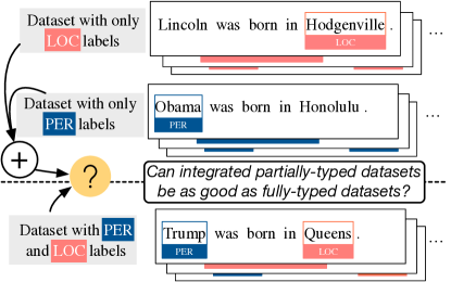
Annotations from different partially-typed datasets are not only incomplete but heterogeneous (different datasets are annotated to different label space). Therefore, special handling is required to integrate these datasets. For example, in Figure 1, only LOC entities are annotated in the first dataset and only PER entities are labeled in the second dataset. Although combining them together provides us annotations for both types of entities, directly merging them together without handling their difference would result in massive label noise (e.g., it teaches the model to annotate Lincoln and other person names as none-entity in the first dataset). Many efforts have been made to mediate different datasets and handle their disparity Scheffer et al. (2001); Mukherjee and Ramakrishnan (2004); Bui et al. (2008); Yu and Joachims (2009); Fernandes and Brefeld (2011); Greenberg et al. (2018); Jie et al. (2019); Beryozkin et al. (2019); Huang et al. (2019). For example, Greenberg et al. (2018) proposes to combine EM marginalization and conditional random field (CRF), which significantly outperforms its directly merging baseline and verifies the need of integration algorithm. However, due to the lack of theory describing the underlying mechanisms and assumptions of the desired integration, it is still not clear on how dataset integration should be conducted, or whether integrated partially-typed datasets can be as good as fully-typed datasets.
Here, we conduct systematic analysis and comparison between partially-typed NER datasets and fully-typed NER datasets. Our main contributions are summarized as follows.
-
•
We conduct theoretical analysis on the potential of partially-typed datasets. We establish that, under certain conditions, model performance of detecting fully-typed entities is bounded by the performance of detecting partially-typed entities. Thus, with partially-typed annotations, the algorithm is able to optimize both a upper bound and a lower bound of the fully-typed performance. Our results not only reveal partially-typed datasets have a similar potential with fully-typed ones but shed insights on the algorithm design.
-
•
We further designed controlled experiments to verify our theoretical analysis. Specifically, we generated simulated partially-typed and fully-typed datasets, implemented various heuristic methods for dataset integration. With the same amount of annotated entities, models trained with partially-typed datasets achieve the comparable performance with ones trained with fully-typed datasets. It matches our theoretical results and verifies the potential of partially-type datasets.
2 Partilly-Typed Dataset Analysis
Here, we conduct analysis on the potential of the partially-typed annotation. Specifically, we aim to understand whether partially-typed datasets can achieve a similar performance with fully-typed datasets. We first describe our problem setting, briefly introduce sequence labeling models, and then proceed to our theoretical results.
2.1 Problem Setting
We consider a collection of annotated NER corpora , where is a corpus with a pre-defined target type set, denoted by . In other words, for , all entities within are labeled with their types and other words are labelled with O, i.e., not-target-type.
We aim to leverage all datasets to train a unified named entity recognizer which can extract entities of any type in . Formally, we define our task as: constructing a single model with to annotate all entities within the complete type set and all other words as O.
2.2 Sequence Labeling
Recently, most NER systems are characterized by sequence labeling models under labeling schemas like IOB and IOBES Ratinov and Roth (2009). In the IOBES schema, when a sequence of tokens is identified as a named entity, its starting, middle and ending tokens are labeled as B-, I-, E-, respectively, followed by the type. If a single word is an entity, it is labeled as S- instead.
To capture the dependency among labels, first-order CRF is widely used in existing NER systems and has crucial impact on the model performance Reimers and Gurevych (2017). Specifically, for input sequence , most models calculate a representation for each token. We refer the representation sequence as , where is the representation of . For an input sequence , CRF defines the conditional probability of as
| (1) |
where is a generic label sequence, is the set of all generic label sequences for and is the potential function. For computation efficiency, the potential function is usually defined as:
where and are the weight and bias term to be learned.
The negative log-likelihood of Equation 1 is treated as the loss function for model training; during inference, the optimal label sequence is found by maximizing the probability in Equation 1. Although is exponential w.r.t. the sentence length, both training and inference can be efficiently completed with dynamic programming algorithms.
2.3 Potential of Partially-typed Datasets
Intuitively, from multiple partially annotated corpora, we could obtain sufficient supervision for training w.r.t. the complete type set . Still, there is no guarantee about the model performance trained with such annotations.
Existing studies about generalization errors show that, model performance w.r.t. is bounded by its performance on the corresponding training set London et al. (2016). Here, we further establish the connection between model performance w.r.t. and the performance w.r.t. . In particular, since typical sequence labeling models treat sentences as the training unit, we use the sentence-level error rate Fernandes and Brefeld (2011) to evaluate the performance w.r.t. .
| (2) |
where is the score calculated by the NER model for the input and label . Specifically, for the CRF model (Equation 1), would be . is an error indicator function, it equals to zero if its condition is false, i.e., the correct label sequence has the highest score; or equals to one otherwise.
Next, we define the partial error rate, which only considers entity prediction within and can be evaluated with the partially-typed dataset . Since only entities within are evaluated, predicted entities with other types need to be omitted. Thus, is defined to replace all annotations in with O and convert into a new label sequence. Then, with regard to a type set , the target label sequence set can be defined as
It is worth mentioning that would result in the same set of sequences no matter whether is fully-typed or partially-typed, thus can be calculated with either fully-typed dataset or . Based on , we define the sentence-level partial error rate w.r.t. as:
| (3) |
Specifically, the error indicator function in Equation 3 would equal to zero if there exists a label sequence in having the highest score among all possible label sequences ; otherwise, it would equal to one. Similar to , would have the same value evaluated on fully-typed datasets and on the partially-typed dataset . To simplify the notation, we use full annotations to calculate both and , then derive their connections as
Theorem 1.
If annotations w.r.t. could determine annotations w.r.t. without any ambiguity, i.e., for . We would have:
Theory 1 shows that, by training model with partially-typed datasets, an algorithm can optimize both the lower bound and the upper bound of the performance for recognizing fully-typed entities.
To prove this theory, we first introduce a lemma. Specifically, We denote the prediction error as:
In this way, we have Similarly, we define , the prediction error within as
and get . Now we can establish the connection between and as follows.
Lemma 1.
If annotations of could determine annotations of without any ambiguity, i.e., , we could have: and , the value of would be equal to .
Proof.
If , we have
Thus for , we have . Then, we have
| (4) |
Now we proceed to prove that, if Equation 4 holds true, we have . For the sake of contradiction, we suppose that satisfies both and Equation 4. Thus, . Since , we have
where . Besides, since we have . Therefore, we have . Thus,
Based on definition, we have , which contradicts to our assumption that Equation 3 holds true.
Hence, if , . Accordingly, and , we have
∎
Now, we proceed to prove the Theorem 1.
Proof.
Since for , thus
Based on the definition, we get and .
Then, we prove the second inequality in Theorem 1. With Lemma 1, we know that, if annotations of could determine annotations of without any ambiguity, we would have . Therefore, we have
which is the second inequality in Theorem 1.
∎
For a quick summary, we establish that, if partially-annotated datasets provide sufficient supervision (i.e., annotations for could determine annotations for without any ambiguity), on the test set can be bounded by on the test set; and based on previous work London et al. (2016), we can bound on the test set with on . In other words, for a list of datasets, if their labeling schemas could determine the annotation for without any ambiguity, partial annotations alone can be sufficient for sequence labeling model training.
It is worth mentioning that our study is the first analyzing the potential of partially-typed datasets for sequence labeling and providing theoretical supports for learning with complementary but partially-typed datasets. We now discuss its connection to the previous work, which studies this problem empirically.
2.4 Connection to Existing Methods
Due to the lack of guidance on theory design, many principles and methods have been leveraged to integrate partially-typed datasets (as introduced in Section 4.2). Jie et al. (2019) shows that EM-CRF or CRF with marginal likelihood training significantly outperforms other principles. Here, we show the connection between our theory and marginal likelihood training.
Connection to Marginal Likelihood Training. As introduced in Section 2.2, the widely used objective function for conventional CRF models is the negative log likelihood:
| (5) |
Equation 5 can be viewed as an approximation to the sentence error rate (i.e., Equation 2). Specifically, if has the largest value among all possible label sequences (the model output is correct), both and Equation 5 would be zero; otherwise (the model output is wrong), would be one and Equation 5 would be positive. Thus, the sentence-level error rate could be viewed as the norm of Equation 5, and the negative log likelihood can be viewed as an approximate of the sentence level error rate.
Since could be bounded by (Theorem 1), it’s intuitive to design the learning objective as minimizing an approximation of for the complementary learning. Specifically, similar to Equation 5, in is approximated as below
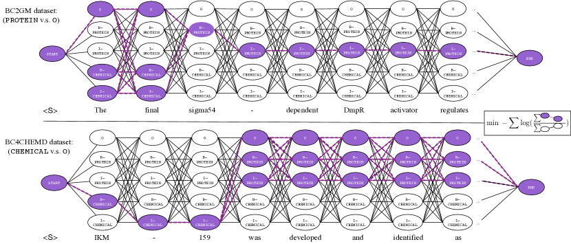
which is the objective for the marginal likelihood training Greenberg et al. (2018); Jie et al. (2019) (as visualized in Fig 2). Similar to Equation 1, it can be calculated efficiently with dynamic programming.
3 Experiments
We further conduct experiments to compare fully-typed datasets with partially-typed ones. We first introduce compared methods, then discuss the empirical results.
3.1 Experiment Setting
We generate simulated partially-typed datases from fully-typed datasets, which allows us to have consistent annotation quality and controllable annotation quantity. Specifically, we first devide a bioNER dataset JNLPBA Crichton et al. (2017) into folds ( in our experiments), preserve one type of entities in each split and mask other entities as O. Statistics of the resulting dataset are summarized in Table 1 and more details are included in the Appendix.
| DNA | protein | cell-type | cell-line | RNA | ||||||
| Sent. | Entity | Sent. | Entity | Sent. | Entity | Sent. | Entity | Sent. | Entity | |
| 3-split | 5571 | 7385 | 5571 | 16729 | 5571 | 4778 | – | – | – | – |
| 4-split | 4178 | 5607 | 4178 | 12720 | 4179 | 3575 | 4178 | 2495 | – | – |
| 5-split | 3343 | 4509 | 3342 | 10189 | 3343 | 2855 | 3342 | 1940 | 3343 | 539 |
3.2 Compared Methods
We implement and conduct experiments with four types of methods. It is worth mentioning that, all methods are based on the same base sequence labeling model as described in Sec 2.2.
Naive Method (Concat). We implement a naive method to demonstrate the difference between our problem to classical supervised learning. Concat naively overlooks the label inconsistency problem and trains a model by directly combining different datasets. As each separate dataset can be viewed as an incompletely labeled corpus w.r.t. the union type space, Concat introduces many false negatives into the training process, undermining the performance of the model.
Marginal Likelihood Training (Partial). As in Figure 2, there may exist multiple valid target sequences in a partially-typed dataset. Therefore, the marginal likelihood training is employed as the learning objective, which seeks to maximize the probability of all possible label sequences Greenberg et al. (2018): . It can be efficiently calculated with dynamic programming.
By maximizing the probability of all label sequences that are consistent with partially-typed labels, the CRF model is allowed to coordinate the label spaces during model learning. For example, in Figure 2, the marginal likelihood training would try to discriminate PROTEIN against other entities in the BC2GM dataset and discriminate CHEMICAL against other entities in the BC2CHEMD dataset. This allows the model to take advantage of the positive labels from each dataset while over-penalize uncertain labels. As a result, the model spontaneously integrates supervision signals from all training sets, having the ability to identify entities of all previously seen types. In the inference process, such model would extract entities of all types.
Label Propagation (Propagate). We design a heuristic strategy to integrate partially-typed datasets by propagating labels. Specifically, we first train separate models, each from a different dataset. Then, we use these models to annotate each other. Thus, each dataset will thus have two types of labels: gold labels come from manual annotation and propagated labels come from models trained with other datasets. Propagate merges original annotations with propagated labels by treating both as the target sequences and the marginal likelihood as the objective for training.
Conventional Supervised Method (Standard♠). We also construct conventional supervised sequence labeling model with sampled datasets. Specifically, Standard♠( sent. w. types) is trained on a fully-typed dataset which has roughly the same amount of annotated entities with -split but less sentences. Standard♠(all sent. w. types) is to train on a fully-typed dataset which has roughly the same amount of sentences with -split but more annotated entities. 1-Type is to train a single-type NER with the access to all annotations of a single type of entities.
3.3 Performance Comparison
| Dataset | Method | Per-type | Micro | ||||
| cell-type | DNA | protein | cell-line | RNA | |||
| 3-split (5571 sent./type) | Concat | 28.24 | 18.72 | 32.95 | – | – | 30.16 |
| Propagate | 71.10 | 71.32 | 75.53 | – | – | 73.85 | |
| Partial | 75.41 | 72.55 | 76.41 | – | – | 75.58 | |
| Standard♠ (5571 sent. w. 3 types) | 72.86 | 68.09 | 73.20 | – | – | 69.62 | |
| Standard♠ (all sent. w. 3 types) | 75.64 | 70.69 | 76.37 | – | – | 75.47 | |
| 4-split (4178 sent./type) | Concat | 17.32 | 25.02 | 24.78 | 16.41 | – | 22.74 |
| Propagate | 69.81 | 67.52 | 73.78 | 55.54 | – | 70.94 | |
| Partial | 76.13 | 70.55 | 75.23 | 61.82 | – | 73.83 | |
| Standard♠ (4178 sent. w. 4 types) | 72.30 | 66.09 | 72.19 | 57.78 | – | 70.09 | |
| Standard♠ (all sent. w. 4 types) | 78.00 | 70.20 | 76.19 | 62.26 | – | 74.96 | |
| 5-split (3343 sent./type) | Concat | 6.99 | 24.58 | 19.41 | 9.68 | 13.95 | 16.89 |
| Propagate | 68.66 | 63.67 | 70.58 | 56.77 | 68.34 | 68.37 | |
| Partial | 73.72 | 71.34 | 74.67 | 60.87 | 72.65 | 73.00 | |
| Standard♠ (3343 sent. w. 4 types) | 74.32 | 66.67 | 71.15 | 59.02 | 63.96 | 70.49 | |
| Standard♠ (all sent. w. 5 types) | 76.71 | 70.64 | 76.31 | 61.08 | 73.07 | 74.75 | |
As shown in Table 2, the Partial model significantly outperforms Concat and Propagate in both per-type and micro . Also, the performance of partially-typed datasets keeps dropping as the number of types grows (since larger results in less annotated entities per type). Among these methods, Concat performs much worse than all other methods due to the effect of false negatives, which verifies the importance of properly integrating datasets. Propagate adds more constraints to the target label set of Partial and achieves worse performance (Partial achieves , , gain over Propagate for , respectively). Such result indicate that it is more profitable not to constraints on the target label space and allow the algorithm to infer the labels in an adaptive manner.
To examine the efficacy of partially-typed datasets, we compare the performance of Partial and Standard♠. Partial obtains much better results than Standard♠ ( sent. w. types), which has less sentences and roughly the same number of annotated entities. At the same time, Partial obtains comparable performance than Standard♠(all sent, types), which has with the same amount of sentences and more annotated entities (comparing to Standard♠(all sent, types), Partial is only trained with annotated entities). Overall, the result verifies the potential of partially-typed datasets and accords with our derivation and matches our theoretical results.
4 Related Work
There exist two aspects of related work regarding the topic here, which are sequence labeling and training with incomplete annotations.
4.1 Sequence Labeling
Most recent approaches to NER have been characterized by the sequence labeling model, i.e., assigning a label to each word in the sentence. Traditional methods leverage handcrafted features to capture linguistic signals and employ conditional random fields (CRF) to model label dependencies Finkel et al. (2005); Settles (2004); Leaman et al. (2008). Many efforts have been made to leverage neural networks for representation learning and free domain experts from handcrafting features Huang et al. (2015); Chiu and Nichols (2016); Lample et al. (2016); Ma and Hovy (2016); Liu et al. (2018). Recent advances demonstrated the great potential of natural language models and extensive pre-training Peters et al. (2018); Akbik et al. (2018); Devlin et al. (2019). However, most methods only leverage one dataset for training, and doesn’t have the ability to handle the inconsistency among datasets.
4.2 Training with Incomplete Annotations
As aforementioned, special handlings are needed to integrate different datasets. To the best of our knowledge, Scheffer et al. (2001) is the first to study the problem of using partially labelled datasets for learning information extraction models. Mukherjee and Ramakrishnan (2004) further incorporates ontologies into HMMs to model incomplete annotations. Bui et al. (2008) extends CRFs to handle this problem, while Yu and Joachims (2009) leverages structured SVMs. Carlson et al. (2009) conduct training with partial perceptron, which only considers typed entities but not none-entity words; transductive perceptron is leveraged to infer labels for all words Fernandes and Brefeld (2011). After neural networks have demonstrated their ability to substantially increase the performance of NER models, attempts have been made to train neural models with partially-typed NER dataset Giannakopoulos et al. (2017); Shang et al. (2018). Greenberg et al. (2018) studies the problem of using multiple partially-typed NER dataset to conduct training. More and more attentions have been attracted to further improve the model performance Jie et al. (2019); Beryozkin et al. (2019); Huang et al. (2019). Our work aims to answer the question whether models trained with partially-typed NER datasets can achieve comparable performances with ones trained with fully-typed NER datasets and how to integrate partially-typed NER datasets.
5 Conlcusion
We study the potential of partially-typed datasets for NER training. Specifically, we theoretically establish that the model performance evaluated with full annotations could be bounded by those with partial annotations. Besides, we reveal the connection from our derivation to marginal likelihood training, which provides guidance on algorithm design. Furthermore we conduct empirical studies to verify our intuition and find experiments match our theoretical results.
There are many interesting directions for future work. For example, for even the same entity type, different real-world datasets may have different definitions or annotation guidelines. It would be beneficial to allow models self-adapt to different label spaces and handle the disparity among different annotation guidelines.
References
- Akbik et al. [2018] Alan Akbik, Duncan Blythe, and Roland Vollgraf. Contextual string embeddings for sequence labeling. In COLING, 2018.
- Beryozkin et al. [2019] Genady Beryozkin, Yoel Drori, Oren Gilon, Tzvika Hartman, and Idan Szpektor. A joint named-entity recognizer for heterogeneous tag-setsusing a tag hierarchy. In ACL, 2019.
- Bui et al. [2008] Hung H Bui, Dinh Q Phung, Svetha Venkatesh, et al. Learning discriminative sequence models from partially labelled data for activity recognition. In Pacific Rim International Conference on Artificial Intelligence, 2008.
- Bunescu and Mooney [2005] Razvan C Bunescu and Raymond J Mooney. A shortest path dependency kernel for relation extraction. In EMNLP, 2005.
- Carlson et al. [2009] Andrew Carlson, Scott Gaffney, and Flavian Vasile. Learning a named entity tagger from gazetteers with the partial perceptron. In AAAI Spring Symposium: Learning by Reading and Learning to Read, 2009.
- Chiu and Nichols [2016] Jason PC Chiu and Eric Nichols. Named entity recognition with bidirectional lstm-cnns. TACL, 2016.
- Crichton et al. [2017] Gamal Crichton, Sampo Pyysalo, Billy Chiu, and Anna Korhonen. A neural network multi-task learning approach to biomedical named entity recognition. BMC bioinformatics, 2017.
- Devlin et al. [2019] Jacob Devlin, Ming-Wei Chang, Kenton Lee, and Kristina Toutanova. Bert: Pre-training of deep bidirectional transformers for language understanding. In NAACL-HLT, 2019.
- Fernandes and Brefeld [2011] Eraldo R Fernandes and Ulf Brefeld. Learning from partially annotated sequences. In ECMLPKDD, 2011.
- Finkel et al. [2005] J. R. Finkel, T. Grenager, and C. Manning. Incorporating non-local information into information extraction systems by Gibbs sampling. In ACL, 2005.
- Giannakopoulos et al. [2017] Athanasios Giannakopoulos, Claudiu Musat, Andreea Hossmann, and Michael Baeriswyl. Unsupervised aspect term extraction with b-lstm & crf using automatically labelled datasets. In WASSA@EMNLP, 2017.
- Greenberg et al. [2018] Nathan Greenberg, Trapit Bansal, Patrick Verga, and Andrew McCallum. Marginal likelihood training of bilstm-crf for biomedical named entity recognition from disjoint label sets. In EMNLP, 2018.
- Guo et al. [2009] Jiafeng Guo, Gu Xu, Xueqi Cheng, and Hang Li. Named entity recognition in query. In SIGIR, 2009.
- Huang et al. [2019] Xiao Huang, Li Dong, Elizabeth Boschee, and Nanyun Peng. Learning a unified named entity tagger from multiple partially annotated corpora for efficient adaptation. In CoNLL, 2019.
- Huang et al. [2015] Zhiheng Huang, Wei Xu, and Kai Yu. Bidirectional lstm-crf models for sequence tagging. arXiv preprint arXiv:1508.01991, 2015.
- Jie et al. [2019] Zhanming Jie, Pengjun Xie, Wei Lu, Ruixue Ding, and Linlin Li. Better modeling of incomplete annotations for named entity recognition. In NAACL-HLT, 2019.
- Lample et al. [2016] Guillaume Lample, Miguel Ballesteros, Sandeep Subramanian, Kazuya Kawakami, and Chris Dyer. Neural architectures for named entity recognition. In NAACL-HLT, 2016.
- Leaman et al. [2008] Robert Leaman, Graciela Gonzalez, et al. Banner: an executable survey of advances in biomedical named entity recognition. In Pacific Symposium on Biocomputing, 2008.
- Liu et al. [2018] Liyuan Liu, Jingbo Shang, Frank Xu, Xiang Ren, Huan Gui, Jian Peng, and Jiawei Han. Empower sequence labeling with task-aware neural language model. In AAAI, 2018.
- London et al. [2016] Ben London, Bert Huang, and Lise Getoor. Stability and generalization in structured prediction. JMLR, 2016.
- Ma and Hovy [2016] Xuezhe Ma and Eduard Hovy. End-to-end sequence labeling via bi-directional lstm-cnns-crf. In ACL, 2016.
- Moen and Ananiadou [2013] SPFGH Moen and Tapio Salakoski2 Sophia Ananiadou. Distributional semantics resources for biomedical text processing. In Proceedings of the 5th International Symposium on Languages in Biology and Medicine, Tokyo, Japan, pages 39–43, 2013.
- Mukherjee and Ramakrishnan [2004] Saikat Mukherjee and IV Ramakrishnan. Taming the unstructured: Creating structured content from partially labeled schematic text sequences. In OTM Confederated International Conferences ”On the Move to Meaningful Internet Systems”, 2004.
- Peters et al. [2018] Matthew E. Peters, Mark Neumann, Mohit Iyyer, Matt Gardner, Christopher Clark, Kenton Lee, and Luke Zettlemoyer. Deep contextualized word representations. In NAACL-HLT, 2018.
- Ratinov and Roth [2009] Lev Ratinov and Dan Roth. Design challenges and misconceptions in named entity recognition. In CoNLL, 2009.
- Reimers and Gurevych [2017] Nils Reimers and Iryna Gurevych. Optimal hyperparameters for deep lstm-networks for sequence labeling tasks. CoRR, abs/1707.06799, 2017.
- Scheffer et al. [2001] Tobias Scheffer, Christian Decomain, and Stefan Wrobel. Active hidden markov models for information extraction. In International Symposium on Intelligent Data Analysis, 2001.
- Settles [2004] Burr Settles. Biomedical named entity recognition using conditional random fields and rich feature sets. In Proceedings of the international joint workshop on natural language processing in biomedicine and its applications, 2004.
- Shang et al. [2018] Jingbo Shang, Liyuan Liu, Xiaotao Gu, Xiang Ren, Teng Ren, and Jiawei Han. Learning named entity tagger using domain-specific dictionary. In EMNLP, 2018.
- Yu and Joachims [2009] Chun-Nam John Yu and Thorsten Joachims. Learning structural svms with latent variables. In ICML, 2009.
Model Training and Hyper-parameters
We choose hyper-parameters based on the previous study Reimers and Gurevych [2017] and use the chosen values for all methods. Specifically, we use 30-dimension character embeddings and 200-dimension pre-trained word embeddings Moen and Ananiadou [2013]. Both LSTMs are bi-directional. Character-level LSTMs are set to be one-layered with 64-dimension hidden states in each direction; word-level ones are set to be two-layer with 50-dimension hidden states in each direction. Dropout with ratio 0.25 is applied to the output of each layer. Stochastic gradient descent with momentum is employed as the optimization algorithm, and the batch size, momentum and learning rate are set to 32, 0.9 and respectively. Here is the initial learning rate and is the decay ratio. For better stability, we set the gradient clipping threshold to 5.
Evaluation Metrics and Data Source
We use entity-level as the evaluation metric. Micro is computed over all types by counting the total true positives, false negatives and false positives. Per-type is calculated by counts of each type. All datasets we use are collected by Crichton et al. [2017], can be downloaded from Github111https://github.com/cambridgeltl/MTL-Bioinformatics-2016, and the original train, development and test splits are adopted.