Abstract

We introduce two classes of multivariate log skewed distributions with normal kernel: the log canonical fundamental skew-normal (log-CFUSN) and the log unified skew-normal (log-SUN). We also discuss some properties of the log-CFUSN family of distributions. These new classes of log-skewed distributions include the log-normal and multivariate log-skew normal families as particular cases. We discuss some issues related to Bayesian inference in the log-CFUSN family of distributions, mainly we focus on how to model the prior uncertainty about the skewing parameter. Based on the stochastic representation of the log-CFUSN family, we propose a data augmentation strategy for sampling from the posterior distributions. This proposed family is used to analyze the US national monthly precipitation data. We conclude that a high dimensional skewing function lead to a better model fit.

Keywords: skewed distributions; data augmentation; bayesian inference.

AMS 1991 subject classification: 62H05; 62F15; 62E10

1 Introduction

The construction of new parametric distributions has received considerable attention in recent years. This growing interest is motivated by datasets that often present strong skewness, heavy tails, bimodality and some other characteristics that are not well fitted by the usual distributions, such as the normal, Student-$t$, log-normal, exponential and many others. The main goal is to build more flexible parametric distributions with additional parameters allowing to control such characteristics. If compared to finite mixtures of distributions (see Lin et al., 2007b; Cabral et al., 2008, for instance) or nonparametric methods (for recent surveys on Bayesian nonparametric see Müller and Quintana, 2004; Walker, 2005; Dey et al., 1998), one advantage of this approach is that, in general, more parsimonious models are obtained and, as a consequence, the inference process tends to become simpler.

It is not feasible to mention all developments in this area in recent years. Arnold and Beaver (2002), Genton (2004) and Azzalini (2005) review several recent works in the area and are important sources of a detailed discussion of such distributions properties. Further advances in the area can be found in Genton and Loperfido (2005), Arellano-Valle and Azzalini (2006), Arellano-Valle et al. (2006), Arnold et al. (2009), Elal-Olivero et al. (2009), Arellano-Valle et al. (2010), Marchenko and Genton (2010), Goméz et al. (2011), Bolfarine et al. (2011), Rocha et al. (2013) and many others.

The seminal paper by Azzalini (1985) is one of the main references in this topic and has inspired many other works. Azzalini (1985) introduced the so called skew-normal (SN) family of distributions which probability density function (pdf) is

$$f(z\mid\mu,\omega,\alpha)=\frac{2}{\omega}\phi\left(\frac{z-\mu}{\omega}\right)\Phi\left(\alpha\left(\frac{z-\mu}{\omega}\right)\right),\,\,z\in\mathbb{R},$$ (1)

where $\mu\in\mathbb{R}$ and $\omega\in\mathbb{R}^{+}$ are the location and scale parameters, respectively, $\alpha\in\mathbb{R}$ is the skewness parameter and $\phi$ and $\Phi$ denote, respectively, the pdf and the cumulative distribution function (cdf) of the $N(0,1)$. The family in (1) extends the normal one by introducing an extra parameter to control the asymmetry of the distribution and has the normal family as a particular subclass whenever $\alpha$ equals zero. It also preserves some nice properties of the normal family. Another extension of the univariate distribution in (1) recently appeared in Martinez-Flores et al. (2014) which introduced the so called skew-normal alpha-power distibution. The multivariate analog of the SN distribution was introduced by Azzalini and Dalla Valle (1996).

In a more general setting, Genton and Loperfido (2005) introduced the class of generalized multivariate skew elliptical (GSE) distributions which pdf is

$$f(\mathbf{z}|Q)=2f_{k}(\mathbf{z})Q(\mathbf{z}),\,\,\mathbf{z}\in\mathbb{R}^{k},$$ (2)

where $f_{k}$ is the pdf of a $k$-dimensional elliptical distribution and $Q$ is a skewing function satisfying $Q(-\mathbf{z})=1-Q(\mathbf{z})$, for all $\mathbf{z}\in\mathbb{R}^{k}$. Many of the SN distribution properties also follow to any distribution in this class. Particularly, Genton and Loperfido (2005) prove that distributions of quadratic forms in the GSE family do not depend on the skewing function $Q$. Some other properties of the GSE family, such as the joint moment generating functions of linear transformations and quadratic forms of ${\bf Z}$ and the conditions for their independence, can be found in Huang et al. (2013). It should be also mentioned that the multivariate SN families of distributions defined by Azzalini and Dalla Valle (1996) and Azzalini and Capitanio (1999) and the family of skew-spherical (elliptical) distributions defined in Branco and Dey (2001) are subclasses of (2).

Azzalini and Dalla Valle (1996)’s family of distributions is also a subclass of the fundamental SN (FUSN) class of distributions defined by Arellano-Valle and Genton (2005). A vector $Z^{*}$ has a $n$-variate canonical fundamental skew-normal (CFUSN) distribution with an $n\times m$ skewness matrix $\Delta$, which will be denoted by $Z^{*}\sim CFUSN_{n,m}(\mbox{\boldmath$\Delta$})$, if its density is given by

$$f_{{\bf Z}^{*}}(\mathbf{z})=2^{m}\phi_{n}(\mathbf{z})\Phi_{m}(\mbox{\boldmath$\Delta$}^{\prime}\mathbf{z}|{\bf{I}}_{m}-\mbox{\boldmath$\Delta$}^{\prime}\mbox{\boldmath$\Delta$}),\,\,\,\,\mathbf{z}\in\mathbb{R}^{n},$$ (3)

where $\Delta$ is such that $||\mbox{\boldmath$\Delta$}\mathbf{a}||<1$, for all unitary vectors $\mathbf{a}\in\mathbb{R}^{m}$, and $||^{.}||$ denotes euclidean norm. Along this paper, we denote by $\phi_{n}({\mathbf{y}}\mid{\mathbf{\mbox{\boldmath$\mu$}}},{\mathbf{\Sigma}})$ the p.d.f. associated with the multivariate $N_{n}({\mathbf{\mbox{\boldmath$\mu$}}},{\mathbf{\Sigma}})$ distribution, and by $\Phi_{n}({\mathbf{y}}\mid{\mathbf{\mbox{\boldmath$\mu$}}},{\mathbf{\Sigma}})$ the corresponding cumulative distribution function (c.d.f.). If $\mathbf{\mbox{\boldmath$\mu$}}={\mathbf{0}}$ (respectively $\mathbf{\mbox{\boldmath$\mu$}}={\mathbf{0}}$ and ${\mathbf{\Sigma}}={\bf{I}}_{n}$) these functions will be denoted by $\phi_{n}({\mathbf{y}}\mid{\mathbf{\Sigma}})$ and $\Phi_{n}({\mathbf{y}}\mid{\mathbf{\Sigma}})$ (respectively $\phi_{n}({\mathbf{y}})$ and $\Phi_{n}({\mathbf{y}})$). For simplicity, $\phi({y})$ and $\Phi({y})$ will be used in the univariate case.

Several classes of SN distributions were defined in the literature. An unification of these families is proposed by Arellano-Valle and Azzalini (2006) which define the unified skew-normal family of distribution, the so-called SUN family. A random vector $Z^{*}\sim SUN_{n,m}(\mbox{\boldmath$\eta$},\mbox{\boldmath$\gamma$},\bar{\mbox{\boldmath$\omega$}},\mbox{\boldmath$\Omega$}^{*})$ if its pdf is

$$f_{{\bf Z}^{*}}(\mathbf{z})=\phi_{n}(\mathbf{z}-\mbox{\boldmath$\eta$}\mid\mbox{\boldmath$\Omega$})\frac{\Phi_{m}(\mbox{\boldmath$\gamma$}+\mbox{\boldmath$\Delta$}^{\prime}\bar{\mbox{\boldmath$\Omega$}}^{-1}\mbox{\boldmath$\omega$}^{-1}(\mathbf{z}-\mbox{\boldmath$\eta$})|\mbox{\boldmath$\Gamma$}-\mbox{\boldmath$\Delta$}^{\prime}\bar{\mbox{\boldmath$\Omega$}}^{-1}\mbox{\boldmath$\Delta$})}{\Phi_{m}(\mbox{\boldmath$\gamma$}\mid\mbox{\boldmath$\Gamma$})},\,\,\,\,\mathbf{z}\in\mathbb{R}^{n},$$ (4)

where the vectors $\mbox{\boldmath$\eta$}\in\mathbb{R}^{n}$ and $\mbox{\boldmath$\gamma$}\in\mathbb{R}^{m}$, $\bar{\mbox{\boldmath$\omega$}}$ is the vector of the diagonal elements of $\omega$, $\omega$ is a diagonal matrix formed by the standard deviations of $\mbox{\boldmath$\Omega$}=\mbox{\boldmath$\omega$}\bar{\mbox{\boldmath$\Omega$}}\mbox{\boldmath$\omega$}$, $\bar{\mbox{\boldmath$\Omega$}}$, $\Gamma$ and $\Delta$ are, respectively, $n\times n$, $m\times m$ and $n\times m$ matrices such that

$$\mbox{\boldmath$\Omega$}^{*}=\left(\begin{array}[]{cc}\mbox{\boldmath$\Gamma$}&\mbox{\boldmath$\Delta$}^{\prime}\\ \mbox{\boldmath$\Delta$}&\bar{\mbox{\boldmath$\Omega$}}\\ \end{array}\right)$$

is a correlation matrix. For another unification of multivariate skewed distributions see Abtahi and Towhidi (2013).

In limit cases, some of these distributions concentrate their probability mass in positive (or negative) values. The half-normal distribution, for instance, is obtaind from (1) by assuming $\alpha$ equal to infinite. Because of this, such family of distributions has also been considered to model data with positive support, such as income, precipitation, pollutants concentration and so on. However, such limit distributions are not flexible enough to accommodate the diversity of shapes of positive (or negative) data. In the univariate context, Gamma, exponential and log-normal distributions are commonly used to model non-negative random variables. Less conventional analysis can be done using the log-SN and log-Skew-$t$ introduced by Azzalini et al. (2003) or the log-power-normal distribution introduced by Martinez-Flores et al. (2012).

In the multivariate context, however, distributions with positive support are usually intractable, with the exception of the multivariate log-normal distribution. With the above problem in mind, Marchenko and Genton (2010) built the multivariate log-skew elliptical family of distributions as follows. Denote by $El_{n}(\mathbf{\mu},\mathbf{\Sigma},g^{(n)})$ the family of $n$-dimensional elliptical distributions (with existing pdf) with generating function $g^{(n)}(u),u\geq 0$, defining a $n$-dimensional spherical density, a location column vector $\mathbf{\mu}\in\mathbb{R}^{n}$, and a $n\,$x$\,n$ positive definite dispersion matrix $\mathbf{\Sigma}$. If $\mathbf{X}\sim El_{n}(\mathbf{\mu},\mathbf{\Sigma},g^{(n)})$, then its pdf is $f_{n}(\mathbf{x};\mathbf{\mu},\mathbf{\Sigma},g^{(n)})=|\mathbf{\Sigma}|^{-\frac{1}{2}}g^{(n)}(Q_{\mathbf{x}}^{\mathbf{\mu},\mathbf{\Sigma}})$, where $Q_{\mathbf{x}}^{\mathbf{\mu},\mathbf{\Sigma}}=(\mathbf{x}-\mathbf{\mu})^{\prime}\mathbf{\Sigma}^{-1}(\mathbf{x}-\mathbf{\mu})$, $\mathbf{x}\in\mathbb{R}^{n}$ (Fang et al., 1990). Consider the class of skew elliptical distributions with pdf given by

$$f_{SEl_{n}}(\mathbf{x})=2f_{n}(\mathbf{x};\mathbf{\mu},\mathbf{\Sigma},g^{(n)})F(\mathbf{\alpha^{\prime}}\mathbf{\omega^{-1}}(\mathbf{x}-\mathbf{\mu});g_{Q_{\mathbf{x}}^{\mathbf{\mu},\mathbf{\Sigma}}}),\,\,\mathbf{x}\in\mathbb{R}^{n},$$ (5)

where $\mathbf{\alpha}\in\mathbb{R}^{n}$ is a shape parameter, $\mathbf{\omega}=diag(\mathbf{\Sigma})^{1/2}$ is a $n\,$x$\,n$ scale matrix, $f_{n}(\mathbf{x};\mathbf{\mu},\mathbf{\Sigma},g^{(n)})$ is the pdf of a $n$-dimensional random vector of $El_{n}(\mathbf{\mu},\mathbf{\Sigma},g^{(n)})$ and $F(u;g_{Q_{\mathbf{x}}^{\mathbf{\mu},\mathbf{\Sigma}}})$ is the cdf of the $El_{1}(0,1,g_{Q_{\mathbf{x}}^{\mathbf{\mu},\mathbf{\Sigma}}})$ with generating function $g_{Q_{\mathbf{x}}^{\mathbf{\mu},\mathbf{\Sigma}}}(u)=g^{(n+1)}(u+Q_{\mathbf{x}}^{\mathbf{\mu},\mathbf{\Sigma}})/g^{(n)}(Q_{\mathbf{x}}^{\mu,\Sigma})$. The distribution in (5) is denoted by $SEl_{n}(\mathbf{\mu},\mathbf{\Sigma},\mathbf{\alpha},g^{(n+1)})$. Consider the transformation ${\exp(\mathbf{X})}=(\exp(X_{1}),\dots,\exp(X_{n}))$, where $\mathbf{X}\sim SEl_{n}(\mathbf{\mu},\mathbf{\Sigma},\mathbf{\alpha},g^{(n+1)})$. Then, $\mathbf{X}$ has log-skew elliptical distribution denoted by $\mathbf{X}\sim LSEl_{n}(\mathbf{\mu},\mathbf{\Sigma},\mathbf{\alpha},g^{(n+1)})$ with pdf

$$f_{LSEl_{n}}(\mathbf{x})=2\left(\prod_{i=1}^{n}{x_{i}}\right)^{-1}f_{n}(\ln(\mathbf{x});\mathbf{\mu},\mathbf{\Sigma},g^{(n)})F(\mathbf{\alpha^{\prime}}\mathbf{\omega^{-1}}(\ln(\mathbf{x})-\mathbf{\mu});g_{Q_{\mathbf{x}}^{\mathbf{\mu},\mathbf{\Sigma}}}),\ \mathbf{x}>0.$$ (6)

It is immediate that the multivariate skew-normal (Azzalini and Dalla Valle, 1996) and skew-t (Azzalini and Capitanio, 2003) distributions are special cases of (5). Consequently, the log-skewed class of distributions in (6) introduced by Marchenko and Genton (2010) also defines particular classes of multivariate log-SN and log-skew-$t$ distributions and has, as a special case, the multivariate log-normal family of distributions.

Our main motivation to introduce new classes of multivariate log-skewed distribution are some results that recently appeared in a paper by Santos et al. (2013). That paper focused on the parameter interpretation in the mixed logistic regression models which is done through the so called odds ratio as in the usual logistic regression model. However, by considering the random effects, the odds ratio to compare two individuals in two different clusters becomes a random variable ($OR$) that depends on the random effects related to the two clusters under comparison (Larsen et al., 2000). Because of this, Larsen et al. (2000) propose to interpret the odds ratio in terms of the median of its distribution in order to quantify appropriately the heterogeneity among the different clusters. If the random effects are independent and identically distributed (iid) with $SN(\xi,\sigma^{2},\lambda)$ then Santos et al. (2013) prove that the odds ratio has distribution with pdf given by

$$f_{OR|\mbox{\boldmath$\beta$},\mbox{\boldmath$\theta$},{\bf x}}(r)=\frac{4}{r}\phi(\ln{r}|\kappa_{12},2\sigma^{2})\times\Phi_{2}\left(\frac{\delta\ln{r}}{2\sigma}\mbox{\boldmath$\epsilon$}|\frac{\delta\kappa_{12}}{2\sigma}\mbox{\boldmath$\epsilon$},{\bf{I}}_{2}-\frac{\delta^{2}}{2}\mbox{\boldmath$\epsilon$}\mbox{\boldmath$\epsilon$}^{\prime}\right),\;\;r\in\mathbb{R}_{+},$$ (7)

where $\kappa_{12}=({\bf x}^{\prime}_{i_{1}j_{1}}-{\bf x}^{\prime}_{i_{2}j_{2}})\mbox{\boldmath$\beta$}$, $\mbox{\boldmath$\epsilon$}=(1,-1)^{\prime}$ and $\delta=\lambda(1+\lambda^{2})^{-0.5}$. Similar distributions were also obtained under independent skew-normally distributed random effects. The univariate log-skewed distribution in (7) does not belong to the class of distributions defined by Marchenko and Genton (2010), nor to that introduced by Azzalini et al. (2003). Moreover, only its median was obtained by Santos et al. (2013) but no other property of it was studied.

In this paper, we introduce the multivariate log-CFUSN and log-SUN family of distributions. We explore their relationship and study some properties of the log-CFUSN family of distributions. Such classes of distributions have as subclasses the multivariate log-skew-normal family introduced by Marchenko and Genton (2010), the log-SN family by Azzalini et al. (2003) and the family of distributions given in (7). We also discuss some issues related to Bayesian inference in this family. To illustrate its use we analyze the USA monthly precipitation data recorded from 1895 to 2007, that is available at the National Climatic Data Center (NCDC).

This paper is organized as follows. In Section 2 we define the log-CFUSN and the log-SUN families of distributions and establish some of the probabilistic properties of the log-CFUSN family of distributions. Bayesian inference in the log-CFUSN family is discussed in Section 3. In Section 4 we present some data analysis using the proposed log-CFUSN family of distributions. Finally, Section 5 finishes the paper with a discussion and our main conclusions.

2 Log-SUN and Log-CFUSN families of distributions

Under the normal theory, the log-normal family of distributions is obtained assuming the logarithimic transformation. If a random variable $Y$ is log-normally distributed it follows that the log transformation of it, that is, $X=\ln Y$, has a normal distribution. Following this idea, in this section, we formally define the log-canonical-fundamental-skew-normal (log-CFUSN) and the log-unified-skew-normal (log-SUN) families of distributions and explore some properties of the log-CFUSN such as conditional and marginal distributions, mixed moments and stochastic representations.

Let ${\bf Z}^{*}=(Z^{*}_{1},\dots,Z^{*}_{n})^{\prime}$ be an $n\times 1$ random vector and consider the transformations ${\exp({\mathbf{Z}}^{*})}=(\exp(Z^{*}_{1}),\dots,\exp(Z^{*}_{n}))^{\prime}$ and ${\ln{\mathbf{Z}}^{*}}=(\ln Z^{*}_{1},\dots,\ln Z^{*}_{n})^{\prime}$.

Definition 1.

(Log-CFUSN family of distributions) Let ${\bf Z}^{*}$ and ${\bf Y}$ be $n\times 1$ random vectors such that ${\bf Z}^{*}=\ln{\bf Y}$. We say that ${\bf Y}$ has a log-canonical-fundamental-skew-normal distribution with $n\times m$ skewness matrix $\mathbf{\Delta}$ denoted by $\mathbf{Y}\sim LCFUSN_{n,m}(\mathbf{\Delta})$, if $\mathbf{Z^{*}}\sim CFUSN_{n,m}(\mathbf{\Delta})$ with pdf given in (3).

Thus, from definition 1, we have that $\mathbf{Y}={\exp({\mathbf{Z}}^{*})}$ and using some results of probability calculus, we can prove that the pdf of the log-CFUSN family of distributions with skewness matrix $\mathbf{\Delta}$ is

$$f_{\mathbf{Y}}(\mathbf{y})=2^{m}\left(\prod_{i=1}^{n}y_{i}\right)^{-1}\phi_{n}(\ln\mathbf{y})\Phi_{m}(\mathbf{\Delta}^{\prime}\ln\mathbf{y}|{\bf{I}}_{m}-\mathbf{\Delta}^{\prime}\mathbf{\Delta}),\,\,\,\,\mathbf{y}\in\mathbb{R}^{n^{+}},$$ (8)

where $\mathbf{\Delta}$ is an $n\times m$ matrix such that $||\mathbf{\Delta}\textbf{a}||<1$, for all unity vectors a $\in\mathbb{R}^{m}$.

This distribution generalizes the multivariate log-SN distribution defined by Marchenko and Genton (2010) by assuming a $m$-variate skewing function. If in (8) we take $m=1$ and assume $\mathbf{\alpha}=({\bf{I}}_{m}-\mathbf{\Delta}^{\prime}\mathbf{\Delta})^{-\frac{1}{2}}\mathbf{\Delta}^{\prime}$ we obtain the family defined by Marchenko and Genton (2010) which general expression is given in $(\ref{logskewelliptical})$. If $\mathbf{\Delta}$ is a matrix with all entries equal to zero we have the multivariate log-normal distribution. Another reason to study this distribution comes from results in Santos et al. (2013) summarized in the introduction. As it can be noticed, the distribution for the odds ratio given in (7) also belongs to the log-CFUSN family of distributions whenever the individuals under comparison have the same characteristics, that is, equal vector of covariates (${\bf x}^{t}_{i_{1}j_{1}}={\bf x}^{t}_{i_{2}j_{2}}$), and the scale parameter for the distribution of the random effects is $\sigma^{2}=1$. In that case, $OR\sim LCFUSN_{1,2}(\mathbf{\Delta})$ where $\mathbf{\Delta}=\delta\mbox{\boldmath$\epsilon$}$.

Figure 1 depicts the densities of $LCFUSN_{n,m}(\mathbf{\Delta})$ for the case $n=1$ and some values of $m$ and $\mathbf{\Delta}$. To simplify the presentation let ${\bf{1}}_{n,m}$ be the matrix of ones of order $n\times m$ and denote by ${\bf{1}}_{n}$ the column vector of ones of order $n$. Clearly the distribution allocates more mass to the tails when $m$ increases. Moreover, the densities shape becomes more flexible if compared with (6).

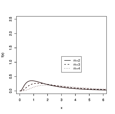
Figure 1: Log-CFUSN densities $LCFUSN_{1,m}(\mathbf{\Delta})$ for different values of $m$ and $\mathbf{\Delta}=0.4\times{\bf{1}}_{m}^{\prime}$ (left) and $\mathbf{\Delta}=-0.4\times{\bf{1}}_{m}^{\prime}$ (right).

In order to show the effect of $m$ in the asymmetry of the distribution, Figures 3 and 3 show the contour plots for the log-CFUSN densities $LCFUSN_{n,m}(\mathbf{\Delta})$ whenever $m=2$ and $3$, respectively. In both cases we assume bivariate ($n=2$) log-CFUSN densities. In Figure 3 the following skewness matrices of parameters $\mathbf{\Delta}$ are assumed $\mathbf{\Delta}_{1}=-\mathbf{\Delta}_{4}=0.3\times{\bf{1}}_{2,2}$, $\mathbf{\Delta}_{2}=-\mathbf{\Delta}_{5}=0.1\times{\bf{1}}_{2,2}$ and $\mathbf{\Delta}_{3}=-\mathbf{\Delta}_{6}=\left(\begin{array}[]{cc}0.4&0.8\\ 0.3&0.3\end{array}\right)$. In Figure 3 the skewness matrices of parameters $\mathbf{\Delta}$ are $\mathbf{\Delta}_{1}=-\mathbf{\Delta}_{4}=0.3\times{\bf{1}}_{2,3}$, $\mathbf{\Delta}_{2}=-\mathbf{\Delta}_{5}=0.2\times{\bf{1}}_{2,3}$, $\mathbf{\Delta}_{3}=0.1\times{\bf{1}}_{2,3}$ and $\mathbf{\Delta}_{6}=\left(\begin{array}[]{ccc}-0.1&-0.3&-0.2\\ -0.1&-0.3&-0.2\end{array}\right)$.

It is clear that the curves in Figures 3 and 3 deviate from the origin when the entries of $\mathbf{\Delta}$ are positive and curves are more concentrated around the origin when these entries are negative. Similar behavior is noted in the contour curves of the $CFUSN_{n,m}(\mbox{\boldmath$\Delta$})$ distribution in Arellano-Valle and Genton (2005).

Figure 2: Contour plots for the log-CFUSN densities with $n=m=2$ and $\mathbf{\Delta_{1}}$ (top left), $\mathbf{\Delta_{2}}$ (top middle), $\mathbf{\Delta_{3}}$ (top right), $\mathbf{\Delta_{4}}$ (bottom left), $\mathbf{\Delta_{5}}$ (bottom middle), $\mathbf{\Delta_{6}}$ (bottom right).

Figure 3: Contour plots for the log-CFUSN densities with $n=2$ and $m=3$ and $\mathbf{\Delta_{1}}$ (top left), $\mathbf{\Delta_{2}}$ (top middle), $\mathbf{\Delta_{3}}$ (top right), $\mathbf{\Delta_{4}}$ (bottom left), $\mathbf{\Delta_{5}}$ (bottom middle), $\mathbf{\Delta_{6}}$ (bottom right).

It must be also noticed that the log-CFUSN family of distributions is a subclass of an extended class of log-skewed distributions with normal kernel which can be built similarly from the family defined by Arellano-Valle and Azzalini (2006). If we consider the SUN family of distribution in (4), we can define the log-SUN family of distibution as follows.

Definition 2.

(Log-SUN family of distributions) Let ${\bf Z}^{*}$ and ${\bf Y}$ be $n\times 1$ random vectors such that ${\bf Z}^{*}=\ln{\bf Y}$. We say that ${\bf Y}$ has a log-unified-skew-normal distribution with parameters $\eta$, $\gamma$, $\bar{\mbox{\boldmath$\omega$}}$ and $\mbox{\boldmath$\Omega$}^{*}$ as defined in (4) denoted by $\mathbf{Y}\sim LSUN_{n,m}(\mbox{\boldmath$\eta$},\mbox{\boldmath$\gamma$},\bar{\mbox{\boldmath$\omega$}},\mbox{\boldmath$\Omega$}^{*})$, if $Z^{*}\sim SUN_{n,m}(\mbox{\boldmath$\eta$},\mbox{\boldmath$\gamma$},\bar{\mbox{\boldmath$\omega$}},\mbox{\boldmath$\Omega$}^{*})$ with pdf given in (4).

It follows, as a consequence of Definition 2, that the pdf of ${\bf Y}$ is given by

$$f_{{\bf Y}}(\mathbf{y})=\left(\prod_{i=1}^{n}y_{i}\right)^{-1}\phi_{n}(\ln{{\bf y}}-\mbox{\boldmath$\eta$}\mid\mbox{\boldmath$\Omega$})\frac{\Phi_{m}(\mbox{\boldmath$\gamma$}+\mbox{\boldmath$\Delta$}^{\prime}\bar{\mbox{\boldmath$\Omega$}}^{-1}\mbox{\boldmath$\omega$}^{-1}(\ln{{\bf y}}-\mbox{\boldmath$\eta$})|\mbox{\boldmath$\Gamma$}-\mbox{\boldmath$\Delta$}^{\prime}\bar{\mbox{\boldmath$\Omega$}}^{-1}\mbox{\boldmath$\Delta$})}{\Phi_{m}(\mbox{\boldmath$\gamma$}\mid\mbox{\boldmath$\Gamma$})},\,\,\,\,$$ (9)

for $\mathbf{y}\in\mathbb{R}^{n}_{+}.$

Particularly, if $\mathbf{Y}\sim LSUN_{n,m}(\bf{0},\bf{0},{\bf{1}}_{n},\mbox{\boldmath$\Omega$}^{*})$, where ${\bf{1}}_{n}$ is the column vector of ones of order $n$ and $\mbox{\boldmath$\Omega$}^{*}=\left(\begin{array}[]{cc}\mbox{\boldmath$I$}_{m}&\mbox{\boldmath$\Delta$}^{\prime}\\ \mbox{\boldmath$\Delta$}&\mbox{\boldmath$I$}_{n}\\ \end{array}\right),$ it follows that $\mathbf{Y}\sim LCFUSN_{n,m}(\mathbf{\Delta})$ with pdf given in (8).

2.1 Some properties of the Log-CFUSN family of distributions

We now present several properties of the log-CFUSN family of distributions, among them are the mixed moments, the cdf and, marginal and conditional distributions. We also establish conditions for independence in the log-CFUSN family of distributions. Proposition 1 provides the cdf for this family.

Proposition 1.

If $\mathbf{Y}\sim LCFUSN_{n,m}(\mathbf{\Delta})$, then its cdf is given by

$$F_{\mathbf{Y}}(\mathbf{y})=2^{m}\Phi_{n+m}((\ln\mathbf{y^{\prime}},\mathbf{0}^{\prime})^{\prime}|\mathbf{\Omega}),\;\;\mathbf{y}\in\mathbb{R}^{n^{+}}$$ (10)

where $\mathbf{\Omega}=\left(\begin{array}[]{cc}\mathbf{I}_{n}&-\mathbf{\Delta}\\ -\mathbf{\Delta}^{\prime}&\mathbf{I}_{m}\\ \end{array}\right).$

The proof of Proposition 1 follows from Proposition 2.1 in Arellano-Valle and Genton (2005) by noticing that $P(\mathbf{Y}\leq\mathbf{y})=P(\exp({\mathbf{Z}^{*})}\leq\mathbf{y})=P(\mathbf{Z}^{*}<\ln\mathbf{y})=F_{\mathbf{Z}^{*}}(\ln\mathbf{y})$.

The mixed moments of a random vector $\mathbf{Y}\sim LCFUSN_{n,m}(\mathbf{\Delta})$ can be expressed in terms of the moment generating function of a $CFUSN_{n,m}(\mathbf{\Delta})$ distribution. This can be seen in the following proposition.

Proposition 2.

If $\mathbf{Y}\sim LCFUSN_{n,m}(\mathbf{\Delta})$ and $\mathbf{t}=(t_{1},...,t_{d})^{\prime}$, $t_{i}\in\mathbb{N}$, then the mixed moments of $\mathbf{Y}$ are given by

$$E(\prod_{i=1}^{n}{Y_{i}}^{t_{i}})=2^{m}e^{(1/2)\mathbf{t}^{\prime}\mathbf{t}}\Phi_{m}(\mathbf{\Delta}^{\prime}\mathbf{t}).$$ (11)

The proof of Proposition 2 follows by noticing that $E(\prod_{i=1}^{n}{Y_{i}}^{t_{i}})$ $=$ $E(\prod_{i=1}^{n}e^{{t_{i}}\ln{Y_{i}}})$ $=$ $E(e^{\sum_{i=1}^{n}{t_{i}}\ln{Y_{i}}})$ $=$ $E(e^{\mathbf{t}\ln\mathbf{Y}})$ $=$ $M_{\ln\mathbf{Y}}(\mathbf{t})$. As $\mathbf{Y}\sim LCFUSN_{n,m}(\mathbf{\Delta})$ , we have $\ln\mathbf{Y}\sim CFUSN_{n,m}(\mathbf{\Delta})$. The result follows from Proposition 2.3 in Arellano-Valle and Genton (2005).

Considering the result in $(\ref{mmlcfusn})$, we can calculate the moments of a random vector with distribution $LCFUSN_{n,m}(\mathbf{\Delta})$. For example, if we consider $\mathbf{Y}\sim LCFUSN_{1,m}(\mathbf{\Delta})$, we have that

$$E(Y) = 2^{m}e^{1/2}\Phi_{m}(\mbox{\boldmath$\Delta$})$$

$$E(Y^{2}) = 2^{m}e^{2}\Phi_{m}(2\mbox{\boldmath$\Delta$})$$

$$E(Y^{3}) = 2^{m}e^{9/2}\Phi_{m}(3\mbox{\boldmath$\Delta$})$$

$$E(Y^{4}) = 2^{m}e^{8}\Phi_{m}(4\mbox{\boldmath$\Delta$}).$$

Considering these results it can be proved that the coefficient of asymmetry and kurtosis of $Y\sim LCFUSN_{1,m}(\mbox{\boldmath$\Delta$})$ are given, respectively, by

$$\gamma_{Y}=\frac{e^{3}\Phi_{m}(3\mbox{\boldmath$\Delta$})-2^{m}\Phi_{m}(\mbox{\boldmath$\Delta$})(3e\Phi_{m}(2\mbox{\boldmath$\Delta$})-2\Phi_{m}(\mbox{\boldmath$\Delta$}))}{2^{\frac{m}{2}}(e\Phi_{m}(2\mbox{\boldmath$\Delta$})-2^{m}\Phi^{2}_{m}(\mbox{\boldmath$\Delta$}))^{3/2}},$$ (12)

and

$$\kappa_{Y}=\frac{e^{6}\Phi_{m}(4\mbox{\boldmath$\Delta$})-2^{m}(4e^{3}\Phi_{m}(\mbox{\boldmath$\Delta$})\Phi_{m}(3\mbox{\boldmath$\Delta$})-3.2^{m+1}e\Phi^{2}_{m}(\mbox{\boldmath$\Delta$})\Phi_{m}(2\mbox{\boldmath$\Delta$})+3.2^{2m}\Phi^{4}_{m}(\mbox{\boldmath$\Delta$}))}{2^{m}(e^{2}\Phi^{2}_{m}(2\mbox{\boldmath$\Delta$})-2^{m+1}e\Phi_{m}(2\mbox{\boldmath$\Delta$})\Phi^{2}_{m}(\mbox{\boldmath$\Delta$})+2^{2m}\Phi^{4}_{m}(\mbox{\boldmath$\Delta$}))}.$$ (13)

Consequently, if $m=1$ and $\Delta$ is a matrix with all entries equal to zero, that is, if $Y\sim LN(0,1)$ then $\gamma_{Y}=(2+e)\sqrt{e-1}$ and $\kappa_{Y}=e^{4}+2e^{3}+3e^{2}-3$.

Figure 4 depicts the asymmetry coefficient and kurtosis for the $LCFUSN_{1,1}(\mbox{\boldmath$\Delta$})$ distribution. Observe that $\mbox{\boldmath$\Delta$}=0$ corresponds to the log normal case. It is clear, at least in the case $n=m=1$, that asymmetry and kurtosis can change significantly depending on the choice of $\Delta$.

Figure 4: Asymmetry (left) and Kurtosis (right) for the $LCFUSN_{1,1}(\mbox{\boldmath$\Delta$})$ distribution.

Table 1 displays the asymmetry and kurtosis coefficients of the $LCFUSN_{1,m}(\mbox{\boldmath$\Delta$})$ as a function of $m$ and it suggests a monotonic decreasing behavior of these quantities as $m$ increases. Although the behavior of these coefficients depends on $\Delta$, particularly, for $\mbox{\boldmath$\Delta$}=0.4\times{\bf{1}}_{m}^{\prime}$ and $\mbox{\boldmath$\Delta$}=-0.4\times{\bf{1}}_{m}^{\prime}$ the asymmetry and kurtosis coefficients of the $LCFUSN_{1,m}(\Delta)$ are both smaller than those obtained for the $LN(0,1)$ for all $m$ considered in the study.

Table 1: Kurtosis and asymmetry for the $LCFUSN_{1,m}(\mbox{\boldmath$\Delta$})$.

		$\mbox{\boldmath$\Delta$}=0.4\times{\bf{1}}_{m}^{\prime}$			$\mbox{\boldmath$\Delta$}=-0.4\times{\bf{1}}_{m}^{\prime}$
$m$		Kurtosis	Asymmetry		Kurtosis	Asymmetry.
1		$92.84$	$5.64$		$74.39$	$5.20$
2		$76.30$	$5.16$		$48.38$	$4.33$
3		$63.39$	$4.73$		$31.12$	$3.55$
4		$53.42$	$4.36$		$19.52$	$2.84$
5		$45.91$	$4.05$		$11.59$	$2.14$

Similar to what is observed for the CFUSN family of distributions, the log-CFUSN is closed under marginalization but not under conditioning. The next result establishes that the $LCFUSN_{n,m}(\mathbf{\Delta})$ distribution is closed under marginalization. The proof of this result will be omitted. It follows immediately from Proposition 2.6 in Arellano-Valle and Genton (2005) and Definition 1.

Proposition 3.

Let $\mathbf{Y}\sim LCFUSN_{n,m}(\mathbf{\Delta})$ and consider the partitions $\mathbf{Y}=\left(\mathbf{Y}_{1}^{\prime},\mathbf{Y}_{2}^{\prime}\right)^{\prime}$ and $\mathbf{\Delta}=\left(\mathbf{\Delta}_{1}^{\prime},\mathbf{\Delta}_{2}^{\prime}\right)^{\prime}$, where $\mathbf{Y}_{i}$ and $\mathbf{\Delta}_{i}$ has dimensions $n_{i}\times 1$ and $n_{i}\times m$, respectively, and $n_{1}+n_{2}=n$. Then, for $i=1,2$, $\mathbf{Y}_{i}\sim LCFUSN_{n_{i},m}(\mathbf{\Delta}_{i})$ with pdf given by

$$f_{\mathbf{Y}_{i}}(\mathbf{y}_{i})=2^{m}\left(\prod_{j=1}^{n_{i}}y_{j}\right)^{-1}\phi_{n_{i}}(\ln\mathbf{y}_{i})\Phi_{m}(\mathbf{\Delta}^{\prime}_{i}\ln\mathbf{y}_{i}|\mathbf{I}_{m}-\mathbf{\Delta}^{\prime}_{i}\mathbf{\Delta}_{i}),\mathbf{y}_{i}\in\mathbb{R}^{n_{i}^{+}}.$$ (14)

It is also possible to derive conditions for independence under the log-CFUSN family of distributions by assuming some constraints on the partitions defined in Proposition 3.

Proposition 4.

Let $\mathbf{Y}\sim LCFUSN_{n,m}(\mathbf{\Delta})$ and consider the partitions $\mathbf{Y}=\left(\mathbf{Y}_{1}^{\prime},\mathbf{Y}_{2}^{\prime}\right)^{\prime}$ and $\mathbf{\Delta}=\left(\mathbf{\Delta}_{1}^{\prime},\mathbf{\Delta}_{2}^{\prime}\right)^{\prime}$, where $\mathbf{Y}_{i}$ and $\mathbf{\Delta}_{i}$ has dimensions $n_{i}\times 1$ and $n_{i}\times m$, respectively, and $n_{1}+n_{2}=n$. Let $\mbox{\boldmath$\Delta$}_{i}=(\mbox{\boldmath$\Delta$}_{i,1},\mbox{\boldmath$\Delta$}_{i,2})$, where $\mbox{\boldmath$\Delta$}_{i,j}$ has dimension $n_{i}\times m_{j}$, $j=1,2$, and $m_{1}+m_{2}=m$, $m>1$. Then, under each of the conditions below on the shape matrix $\mathbf{\Delta}$, the random vectors $\mathbf{Y}_{1}$ and $\mathbf{Y}_{2}$ are independent

• $\mathbf{\Delta}_{12}=\mathbf{\Delta}_{21}=\mathbf{0}$ and, in this case, $\mathbf{Y}_{i}\sim LCFUSN_{n_{i},m_{i}}(\mathbf{\Delta}_{ii}),i=1,2$;
  

• $\mathbf{\Delta}_{ii}=\mathbf{0},i=1,2$ and, in this case, $\mathbf{Y}_{1}\sim LCFUSN_{n_{1},m_{2}}(\mathbf{\Delta}_{12})$ e $\mathbf{Y}_{2}\sim LCFUSN_{n_{2},m_{1}}(\mathbf{\Delta}_{21})$.

The proof of Proposition 4 is straightforward from Proposition 2.7 in Arellano-Valle and Genton (2005) and thus is omitted. We now obtain the conditional distributions under the $LCFUSN_{n,m}(\mbox{\boldmath$\Delta$})$ family.

Proposition 5.

Let $\mathbf{Y}\sim LCFUSN_{n,m}(\mathbf{\Delta})$ and consider the partitions $\mathbf{Y}=\left(\mathbf{Y}_{1}^{\prime},\mathbf{Y}_{2}^{\prime}\right)^{\prime}$ and $\mathbf{\Delta}=\left(\mathbf{\Delta}_{1}^{\prime},\mathbf{\Delta}_{2}^{\prime}\right)^{\prime}$, where $\mathbf{Y}_{i}$ and $\mathbf{\Delta}_{i}$ has dimensions $n_{i}\times 1$ and $n_{i}\times m$, respectively, and $n_{1}+n_{2}=n$. Then, the conditional pdf of $\mathbf{Y}_{1}$ given $\mathbf{Y}_{2}=\mathbf{y}_{2}$, $\mathbf{y}_{2}\in\mathbb{R}^{n_{2}^{+}}$ is given by

$$f_{\mathbf{Y}_{1}|\mathbf{Y}_{2}=\mathbf{y}_{2}}(\mathbf{y}_{1})=\left(\prod_{i=j}^{n_{1}}y_{j}\right)^{-1}\phi_{n_{1}}(\ln\mathbf{y}_{1})\frac{\Phi_{m}(\mathbf{\Delta}_{1}^{\prime}\ln\mathbf{y}_{1}|-\mathbf{\Delta}^{\prime}_{2}\ln\mathbf{y}_{2},\mathbf{I}_{m}-\mathbf{\Delta}^{\prime}\mathbf{\Delta})}{\Phi_{m}(\mathbf{\Delta}^{\prime}_{2}\ln\mathbf{y}_{2}|\mathbf{I}_{m}-\mathbf{\Delta}^{\prime}_{2}\mathbf{\Delta}_{2})},\;\;\mathbf{y}_{1}\in\mathbb{R}^{n_{1}^{+}}.$$ (15)

The proof follows from results of probability calculus and by noticing that, given $\mathbf{y}_{2}\in\mathbb{R}^{n_{2}^{+}}$, we have that $\Phi_{m}(\mathbf{\Delta}^{\prime}\ln{{\bf y}}|\mathbf{I}_{m}-\mathbf{\Delta}^{\prime}\mathbf{\Delta})=$ $\Phi_{m}(\mathbf{\Delta}_{1}^{\prime}\ln{{\bf y}}_{1}+\mathbf{\Delta}_{2}^{\prime}\ln{{\bf y}}_{2}|\mathbf{I}_{m}-\mathbf{\Delta}^{\prime}\mathbf{\Delta})=\Phi_{m}(\mathbf{\Delta}_{1}^{\prime}\ln{{\bf y}}_{1}|-\mathbf{\Delta}_{2}^{\prime}\ln{{\bf y}}_{2},\mathbf{I}_{m}-\mathbf{\Delta}^{\prime}\mathbf{\Delta})$.

Notice that the log-CFUSN family of distribution per se is not closed under conditioning. However, if considered as a particular subclass of the log-SUN family of distribution, we notice from (15) and (9) that ${\mathbf{Y}}_{1}\mid{\mathbf{Y}}_{2}={\mathbf{y}}_{2}\sim LSUN_{n,m}({\bf{0}},\mbox{\boldmath$\Delta$}_{2}^{\prime}\ln{\mathbf{y}}_{2},{\bf{1}}_{n_{1}},\mbox{\boldmath$\Omega$}^{*})$, where $\mbox{\boldmath$\Omega$}^{*}=\left(\begin{array}[]{cc}\mbox{\boldmath$I$}_{m}-\mbox{\boldmath$\Delta$}_{2}^{\prime}\mbox{\boldmath$\Delta$}_{2}&\mbox{\boldmath$\Delta$}_{1}^{\prime}\\ \mbox{\boldmath$\Delta$}_{1}&\mbox{\boldmath$I$}_{n_{1}}\\ \end{array}\right).$

2.2 A location-scale extension of the log-CFUSN distribution

More flexible class of distributions are obtained if we are able to include on it location and scale parameters. Usually, this is done considering a linear transformation of a variable with the standard distribution. Assuming this principle, we introduce the location-scale extension of the $LCFUSN_{n,m}$ distribution as follows.

Assume that $\mathbf{X}\sim CFUSN_{n,m}(\mathbf{\Delta})$ and define the linear transformation $\mathbf{W}={\mbox{\boldmath$\mu$}}+\mathbf{\Sigma}^{\frac{1}{2}}\mathbf{X}$, where $\mu$ is an $n\times 1$ vector and $\mathbf{\Sigma}$ is an $n\times n$ positive definite matrix. As shown by Arellano-Valle and Genton (2005), the pdf of $\mathbf{X}$ is

$$f_{\mathbf{W}}(\mathbf{w})=2^{m}|\mathbf{\Sigma}|^{-1/2}\phi_{n}(\mathbf{\Sigma}^{-1/2}(\mathbf{w}-{\mbox{\boldmath$\mu$}}))\Phi_{m}(\mathbf{\Delta}^{\prime}\mathbf{\Sigma}^{-1/2}(\mathbf{w}-{\mbox{\boldmath$\mu$}})|\mathbf{I}_{m}-\mathbf{\Delta}^{\prime}\mathbf{\Delta}),\mathbf{w}\in\mathbb{R}^{n}.$$ (16)

Let us consider the transformation $\mathbf{U}=\exp({\mathbf{W}})$. By definition, $\mathbf{U}$ has a location-scale log-CFUSN distribution denoted by $\mathbf{U}\sim LCFUSN_{n,m}({\mbox{\boldmath$\mu$}},\mathbf{\Sigma},\mathbf{\Delta})$ and its pdf is

$$f_{\mathbf{U}}(\mathbf{u}) = 2^{m}|\mathbf{\Sigma}|^{-1/2}\left(\prod_{j=1}^{n}u_{j}\right)^{-1}\phi_{n}(\mathbf{\Sigma}^{-1/2}(\ln\mathbf{u}-{\mbox{\boldmath$\mu$}}))$$ (17)

$$\times \Phi_{m}(\mathbf{\Delta}^{\prime}\mathbf{\Sigma}^{-1/2}(\ln\mathbf{u}-{\mbox{\boldmath$\mu$}})|\mathbf{I}_{m}-\mathbf{\Delta}^{\prime}\mathbf{\Delta}),\mathbf{u}\in\mathbb{R}^{n^{+}}.$$

It is important to note that if $\Sigma={\rm diag}\{\sigma_{1}^{2},\dots,\sigma_{n}^{2}\}$, that is, if we are skewing an independent $n$-variate normal distribution, the distribution in (17) can be obtained from the log-SUN distribution given in (9) by assuming $\mbox{\boldmath$\eta$}=\mu$, $\mbox{\boldmath$\gamma$}=\bf{0}$, $\bar{\mbox{\boldmath$\omega$}}=(\sigma_{1},\dots,\sigma_{n})$ and $\mbox{\boldmath$\Omega$}^{*}=\left(\begin{array}[]{cc}\mbox{\boldmath$I$}_{m}&\mbox{\boldmath$\Delta$}^{\prime}\\ \mbox{\boldmath$\Delta$}&\mbox{\boldmath$I$}_{n}\\ \end{array}\right),$ that is, we have that $\mathbf{\mathbf{U}}\sim LSUN_{n,m}(\mbox{\boldmath$\mu$},\bf{0},\bar{\mbox{\boldmath$\omega$}},\mbox{\boldmath$\Omega$}^{*})$.

Marginal and conditional distributions in the location-scale log-CFUSN class of distributions are not easily obtainable. However, under some particular structures for $\mathbf{\Sigma}$ we can derive such results. Let $W\sim CFUSN_{n,m}(\mathbf{\mu},\mathbf{\Sigma},\mathbf{\Delta})$, as defined in Expression 2.11 in Arellano-Valle and Genton (2005), and consider the partitions

$$\mathbf{W}=\left(\begin{array}[]{c}\mathbf{W}_{1}\\ \mathbf{W}_{2}\\ \end{array}\right),\mathbf{\Delta}=\left(\begin{array}[]{c}\mathbf{\Delta}_{1}\\ \mathbf{\Delta}_{2}\\ \end{array}\right),\mbox{\boldmath$\mu$}=\left(\begin{array}[]{c}{\mbox{\boldmath$\mu$}}_{1}\\ {\mbox{\boldmath$\mu$}}_{2}\\ \end{array}\right),$$

where $\mathbf{W}_{i}$, ${\mbox{\boldmath$\mu$}}_{i}$ and $\mathbf{\Delta}_{i}$ have dimensions $n_{i}\times 1$, $n_{i}\times 1$ and $n_{i}\times m$, $i=1,2$, respectively, and $n_{1}+n_{2}=n$. Suppose also that $\mathbf{\Sigma}$ is a diagonal matrix such that

$$\mathbf{\Sigma}=\left(\begin{array}[]{cc}\mathbf{\Sigma}_{11}&\textbf{0}\\ \textbf{0}&\mathbf{\Sigma}_{22}\\ \end{array}\right),$$

where $\mathbf{\Sigma}_{ij}$ has dimension $n_{i}\times n_{j}$. Under these conditions, it follows that $\mathbf{U}_{i}=\exp({\mathbf{W}_{i}})\sim LCFUSN({\mbox{\boldmath$\mu$}}_{i},\mathbf{\Sigma}_{ii},\mathbf{\Delta}_{i})$, that is the location-scale log-CFUSN family of distributions preserves closeness under marginalization.

It also follows that the conditional distribution of $\mathbf{U}_{1}|\mathbf{U}_{2}=\mathbf{u}_{2}$ is given by

$$f_{\mathbf{U}_{1}|\mathbf{U}_{2}=\mathbf{u}_{2}}(\mathbf{u}_{1}) = \left(\prod_{j=1}^{n_{1}}u_{j}\right)^{-1}\phi_{n_{1}}(\mathbf{\Sigma}_{11}^{-1/2}(\ln\mathbf{u}_{1}-{\mbox{\boldmath$\mu$}}_{1}))$$

$$\times \frac{\Phi_{m}(\mathbf{\Delta}_{1}^{\prime}\mathbf{\Sigma}_{11}^{-1/2}(\ln\mathbf{u}_{1}-{\mbox{\boldmath$\mu$}}_{1})|-\mathbf{\Delta}_{2}^{\prime}\mathbf{\Sigma}_{22}^{-1/2}(\ln\mathbf{u}_{2}-{\mbox{\boldmath$\mu$}}_{2}),I_{m}-\mathbf{\Delta}^{\prime}\mathbf{\Delta})}{\Phi_{m}(\mathbf{\Delta}_{2}^{\prime}\mathbf{\Sigma}_{22}^{-1/2}(\ln\mathbf{u}_{2}-{\mbox{\boldmath$\mu$}}_{2})|I_{m}-\mathbf{\Delta}_{2}^{\prime}\mathbf{\Delta}_{2})},$$

$\mathbf{u}_{1}\in\mathbb{R}^{n_{1}^{+}}$ and $\mathbf{u}_{2}\in\mathbb{R}^{n_{2}^{+}}$.

2.3 Stochastic representation

Stochastic representations of skewed distributions are useful, for instance, to generate samples from those distributions more easily. They also play a very important role in inference if we are interested in apply MCMC or EM methods.

A stochastic representation of the log-CFUSN family is straightforward from the marginal stochastic representation of the CFUSN family given in Arellano-Valle and Genton (2005).

Assume that ${\bf Z}^{*}\sim CFUSN_{n,m}(\mbox{\boldmath$\Delta$})$, where $||\mbox{\boldmath$\Delta$}^{\prime}{\bf a}||<1$ for any unitary vector ${\bf a}\in\mathbb{R}^{n}$. Let ${\bf D}\sim N_{m}(\bf{0},\mbox{\boldmath$I$}_{m})$, $\mathbf{V}\sim N_{n}(\bf{0},\mbox{\boldmath$I$}_{n})$ where ${\bf D}$ and $\mathbf{V}$ are independent column random vectors of order $m$ and $n$, respectively. Denote by $|{\bf D}|$ the vector $(|D_{1}|,...,|D_{m}|)^{\prime}$. Arellano-Valle and Genton (2005) prove that the marginal representation of ${\bf Z}^{*}$ is

$${\bf Z}^{*}\buildrel d\over{=}\mbox{\boldmath$\Delta$}|{\bf U}|+(\mbox{\boldmath$I$}_{n}-\mbox{\boldmath$\Delta$}\mbox{\boldmath$\Delta$}^{\prime})^{1/2}\mathbf{V}.$$ (19)

If ${\bf Y}\sim LCFUSN_{n,m}(\mbox{\boldmath$\Delta$})$ then its marginal representation follows as a consequence of (19) by noticing that ${\bf Y}\buildrel d\over{=}\exp({{\bf Z}^{*}})$ $\buildrel d\over{=}\exp(\mbox{\boldmath$\Delta$}|{\bf D}|)\exp((\mbox{\boldmath$I$}_{n}-\mbox{\boldmath$\Delta$}\mbox{\boldmath$\Delta$}^{\prime})^{1/2}\mathbf{V})$ $\buildrel d\over{=}\exp(\mbox{\boldmath$\Delta$}|{\bf D}|){\bf T}$, where ${\bf T}$ has a multivariate log-normal distribution with a null location parameter and scale matrix equal to $\mbox{\boldmath$I$}_{n}-\mbox{\boldmath$\Delta$}\mbox{\boldmath$\Delta$}^{\prime}$.

3 Some aspects of Bayesian Inference in the LCFUSN Family

Let ${\bf Y}_{1},\dots,{\bf Y}_{L}\mid\mbox{\boldmath$\mu$},\mbox{\boldmath$\Sigma$},\mbox{\boldmath$\Delta$}\buildrel iid\over{\sim}LCFUSN_{n,m}(\mbox{\boldmath$\mu$},\mbox{\boldmath$\Sigma$},\mbox{\boldmath$\Delta$})$ with pdf given in (17). Define the $L\times n$ matrices ${\bf Y}=({\bf Y}_{1},\dots,{\bf Y}_{L})^{\prime}$ and $\ln{\bf Y}=(\ln{\bf Y}_{1},\dots,\ln{\bf Y}_{L})^{\prime}$. Therefore, it follows that the likelihood function is given by

$$f({\bf Y}\mid\mbox{\boldmath$\mu$},\mbox{\boldmath$\Sigma$},\mbox{\boldmath$\Delta$}) = 2^{Lm}\prod_{l=1}^{L}\prod_{j=1}^{n}Y_{lj}^{-1}\phi_{L,n}(\ln{\bf Y}\mid{\bf{1}}_{L}\otimes\mbox{\boldmath$\mu$}^{\prime},{\bf{I}}_{L},\mbox{\boldmath$\Sigma$})$$

$$\times \Phi_{Lm}({\bf{I}}_{L}\otimes\mbox{\boldmath$\Delta$}^{\prime}\mbox{\boldmath$\Sigma$}^{-1/2}vec(\ln{\bf Y})\mid{\bf{1}}_{L}\otimes(\mbox{\boldmath$\Delta$}^{\prime}\mbox{\boldmath$\Sigma$}^{-1/2}\mbox{\boldmath$\mu$}),{\bf{V}}^{*}),$$

where ${\bf{V}}^{*}={\bf{I}}_{Lm}-{\bf{I}}_{L}\otimes\mbox{\boldmath$\Delta$}^{\prime}\mbox{\boldmath$\Delta$}$ and $\mathbf{A}\otimes\mathbf{B}$ denotes the Kronecker product of $\mathbf{A}$ and $\mathbf{B}$, $vec(\cdot)$ is the operator vec and $\phi_{L,n}(\cdot\mid M;C,V)$ denotes the pdf of a matrix-variate normal distribution where $M$ is an $L\times n$ constant vector and $C$ and $V$ are, respectively, $L\times L$ and $n\times n$ constant matrices. Observe that the likelihood function in (3) defines a class of matrix-variate log-CFUSN distributions.

In this work, inference is done under the Bayesian paradigm. Therefore we need to specify prior distributions for all parameters. We consider $m$ as a fixed constant and also assume some usual prior distributions for the location and scale parameters. In the following proposition, we present the posterior full conditional distributions for $\mu$, $\Sigma$ and $\Delta$ whenever the prior distributions for $\mu$, $\Sigma$ are, respectively,

$$\left.\begin{array}[]{rcl}\mbox{\boldmath$\mu$}&\sim&N_{n}(\mbox{\boldmath$\mu$}_{0},\mbox{\boldmath$\Sigma$}_{\mu})\\ \mbox{\boldmath$\Sigma$}&\sim&IW(d,D),\end{array}\right\}$$ (23)

where $\mbox{\boldmath$\mu$}_{0}\in\mathbb{R}^{n}$, $\mbox{\boldmath$\Sigma$}_{\mu}$ is an $n\times n$ symmetric, positive definite matrix, $D$ is an $n\times n$ constant matrix, $d\in\mathbb{R}_{+}$ with $d>n$, and $IW(d,D)$ denotes the inverse-Wishart distribution with parameters $d$ and $D$. A flat prior distribution for $\Sigma$ is obtained by setting $d$ close to zero.

Proposition 6.

Let ${\bf Y}_{1},\dots,{\bf Y}_{L}\mid\mbox{\boldmath$\mu$},\mbox{\boldmath$\Sigma$},\mbox{\boldmath$\Delta$}\buildrel iid\over{\sim}LCFUSN_{n,m}(\mbox{\boldmath$\mu$},\mbox{\boldmath$\Sigma$},\mbox{\boldmath$\Delta$})$. Assume that, a priori, the parameters $\mu$, $\Sigma$ and $\Delta$ are independent and that the prior distributions for $\mu$, $\Sigma$ are given in (23). Suppose $\Delta$ has a proper prior distribution $\pi(\mbox{\boldmath$\Delta$})$. Then, the posterior full conditional distributions for $\mu$, $\Sigma$ and $\Delta$ are given, respectively, by

$$\pi(\mbox{\boldmath$\mu$}\mid\mbox{\boldmath$\Sigma$},\mbox{\boldmath$\Delta$},{\bf Y}) \propto \phi_{n}(\mbox{\boldmath$\mu$}\mid\mbox{\boldmath$\Sigma$}^{*}[\mbox{\boldmath$\Sigma$}_{\mu}^{-1}\mbox{\boldmath$\mu$}_{0}+(\mbox{\boldmath$\Sigma$}^{-1}\otimes{\bf{1}}_{L})^{\prime}vec(\ln{\bf Y})]\mid\mbox{\boldmath$\Sigma$}^{*})$$

$$\times \Phi_{mL}({\bf{I}}_{L}\otimes[{\bf{I}}_{m}-\mbox{\boldmath$\Delta$}^{\prime}\mbox{\boldmath$\Delta$}]^{-1/2}\mbox{\boldmath$\Delta$}^{\prime}\mbox{\boldmath$\Sigma$}^{-1/2}[vec(\ln{\bf Y})-{\bf{1}}_{L}\otimes\mbox{\boldmath$\mu$}])$$

$$\pi(\mbox{\boldmath$\Sigma$}\mid\mbox{\boldmath$\mu$},\mbox{\boldmath$\Delta$},{\bf Y}) \propto {\mathcal{I}}{\mathcal{W}}_{n}(d+L+1,D+[\ln{\bf Y}-{\bf{1}}_{L}\otimes\mbox{\boldmath$\mu$}^{\prime}]^{\prime}[\ln{\bf Y}-{\bf{1}}_{L}\otimes\mbox{\boldmath$\mu$}^{\prime}])$$

$$\times \Phi_{mL}({\bf{I}}_{L}\otimes[{\bf{I}}_{m}-\mbox{\boldmath$\Delta$}^{\prime}\mbox{\boldmath$\Delta$}]^{-1/2}\mbox{\boldmath$\Delta$}^{\prime}\mbox{\boldmath$\Sigma$}^{-1/2}[vec(\ln{\bf Y})-{\bf{1}}_{L}\otimes\mbox{\boldmath$\mu$}])$$

$$\pi(\mbox{\boldmath$\Delta$}\mid\mbox{\boldmath$\mu$},\mbox{\boldmath$\Sigma$},{\bf Y}) \propto \pi(\mbox{\boldmath$\Delta$})\Phi_{mL}({\bf{I}}_{L}\otimes[{\bf{I}}_{m}-\mbox{\boldmath$\Delta$}^{\prime}\mbox{\boldmath$\Delta$}]^{-1/2}\mbox{\boldmath$\Delta$}^{\prime}\mbox{\boldmath$\Sigma$}^{-1/2}[vec(\ln{\bf Y})-{\bf{1}}_{L}\otimes\mbox{\boldmath$\mu$}])$$

where $\mbox{\boldmath$\Sigma$}^{*}=[L\mbox{\boldmath$\Sigma$}^{-1}+\mbox{\boldmath$\Sigma$}_{\mu}^{-1}]^{-1}$ and ${\mathcal{I}}{\mathcal{W}}_{n}(a,A)$ denotes the pdf of the inverse-Wishart distribution with parameters $a$ and $A$.

The proof of Proposition 6 follows by mixing (3), (23) and $\pi(\mbox{\boldmath$\Delta$})$ using the Bayes’s theorem and some well-known results of matrix theory. It is noteworthy that the posterior full conditional distribution of $\mu$ belongs to the SUN family of distributions.

The univariate case is presented in the following corollary. Denote by $IG(\alpha,\beta)$, $\alpha>0$ and $\beta>0$, the inverse-gamma distribution with $E(\sigma^{2})=\alpha(\beta-2)^{-1}$.

Corollary 1.

Let $Y_{1},...,Y_{L}\mid\mu,\sigma,\mbox{\boldmath$\Delta$}\buildrel iid\over{\sim}LCFUSN_{1,m}(\mu,\sigma^{2},\mbox{\boldmath$\Delta$})$ and assume that, a priori, $\mu$, $\sigma$ and $\Delta$ are independent and such that $\mu\sim N(\mu_{0},v)$, $\sigma^{2}\sim IG(\alpha,\beta)$, where $l\in\mathbb{R}$, $v$, $\alpha$ and $\beta$ are non-negative numbers, and $\Delta$ has a proper prior distribution $\pi(\mbox{\boldmath$\Delta$})$. Then, the posterior full conditional distributions for $\mu$, $\sigma$ and $\Delta$ are given, respectively, by

$$f(\mu\mid{\bf y},\sigma^{2},\mbox{\boldmath$\Delta$}) \propto \phi\left(\mu\Big{|}\frac{v^{2}{\bf{1}}_{L}^{\prime}\ln{\bf y}+\mu_{0}\sigma^{2}}{Lv^{2}+\sigma^{2}},\frac{v^{2}\sigma^{2}}{Lv^{2}+\sigma^{2}}\right)$$

$$\times \Phi_{mL}(\sigma^{-1}(\mathbf{I}_{L}\otimes\mbox{\boldmath$\Delta$}^{\prime})(\ln{\bf y}-\mu{\bf{1}}_{L})\mid\mathbf{I}_{mL}-\mathbf{I}_{L}\otimes\mbox{\boldmath$\Delta$}^{\prime}\mbox{\boldmath$\Delta$})$$

$$f(\sigma^{2}\mid{\bf x},\mu,\mbox{\boldmath$\Delta$}) \propto \left(\frac{1}{\sigma^{2}}\right)^{\frac{L+2\alpha+2}{2}}\exp{\left(\frac{2\beta-(\ln{\bf y}-\mu{\bf{1}}_{L})^{\prime}(\ln{\bf y}-\mu{\bf{1}}_{L})}{2\sigma^{2}}\right)}$$

$$\times \Phi_{mL}(\sigma^{-1}(\mathbf{I}_{L}\otimes\mbox{\boldmath$\Delta$}^{\prime})(\ln{\bf y}-\mu{\bf{1}}_{L})\mid\mathbf{I}_{mL}-\mathbf{I}_{L}\otimes\mbox{\boldmath$\Delta$}^{\prime}\mbox{\boldmath$\Delta$})$$

$$f(\mbox{\boldmath$\Delta$}\mid{\bf x},\mu,\sigma^{2}) \propto \pi(\mbox{\boldmath$\Delta$})\Phi_{mL}(\sigma^{-1}(\mathbf{I}_{L}\otimes\mbox{\boldmath$\Delta$}^{\prime})(\ln{\bf y}-\mu{\bf{1}}_{L})\mid\mathbf{I}_{mL}-\mathbf{I}_{L}\otimes\mbox{\boldmath$\Delta$}^{\prime}\mbox{\boldmath$\Delta$}),$$

where $\ln{\bf y}=(\ln y_{1},\dots,\ln y_{L})^{\prime}$.

This result is a straightforward consequence of Proposition 6. It follows by observing that the likelihood function of ${\bf y}$ is given by

$$f({\bf y}|\mu,\sigma^{2},\mbox{\boldmath$\Delta$}) = 2^{Lm}(2\pi\sigma^{2})^{-L/2}\left(\prod_{i=1}^{L}y_{i}\right)^{-1}\exp\left\{-\sum_{i=1}^{L}\frac{(\ln y_{i}-\mu)^{2}}{2\sigma^{2}}\right\}$$

$$\times \prod_{i=1}^{L}\Phi_{m}(\mbox{\boldmath$\Delta$}^{\prime}\sigma^{-1}(\ln y_{i}-\mu)|\mathbf{I}_{m}-\mbox{\boldmath$\Delta$}^{\prime}\mbox{\boldmath$\Delta$}),$$

and that the inverse-Wishart distribution is a generalization of the multivariate inverse-gamma distribution.

Since the parameter $\Delta$ is an $n\times m$ vector with $||\mbox{\boldmath$\Delta$}\textbf{a}||<1$, for all unitary vectors $\textbf{a}\in\mathbb{R}^{m}$, the elicitation of a prior distribution for $\Delta$ becomes a hard task. To overcome this difficulty, we can assume an alternative parametrization of the model by setting $\mbox{\boldmath$\Delta$}=\mbox{\boldmath$\Lambda$}(\mathbf{I}_{m}+\mbox{\boldmath$\Lambda$}^{\prime}\mbox{\boldmath$\Lambda$})^{-1/2}$ for some $n\times m$ real matrix $\Lambda$. A possible prior distribution for $\Lambda$ is a multivariate normal distribution. The calculation of the full conditional distributions under these choices is similar to that presented in Proposition 6 and thus will be omitted. However, we remark that the posterior full conditional distributions for $\mu$ and $\Lambda$ belong to the SUN class of distributions and a skewed inverse-Wishart distribution is the posterior full conditional distribution for $\Sigma$. Consequently, by considering this class of joint prior distributions for $(\mbox{\boldmath$\mu$},\mbox{\boldmath$\Sigma$},\mbox{\boldmath$\Lambda$})$ we have conjugacy. It is notable that we are also performing a conjugate analysis for $(\mbox{\boldmath$\mu$},\mbox{\boldmath$\Sigma$})$ in the cases discussed in Proposition 6 and Corollary 1.

Another way to overcome the problem is to assume $\mbox{\boldmath$\Delta$}=\delta{\bf{1}}_{n,m}$ where $\delta$ is a real number belonging to the interval $(-1,1)$. By carrying this out, the model loses some flexibility. On the other hand we obtain a more parsimonious model which is still able to accommodate different degrees of asymmetry. From now on, we consider this approach and elicit a non-informative uniform prior distribution for $\delta$. Under this more parsimonious model, the posterior full conditional distributions for all parameters follow from Proposition 6 and are given by

$$\pi(\mbox{\boldmath$\mu$}\mid\mbox{\boldmath$\Sigma$},\mbox{\boldmath$\Delta$},{\bf Y}) \propto \phi_{n}(\mbox{\boldmath$\mu$}\mid\mbox{\boldmath$\Sigma$}^{*}[\mbox{\boldmath$\Sigma$}_{\mu}^{-1}\mbox{\boldmath$\mu$}_{0}+(\mbox{\boldmath$\Sigma$}^{-1}\otimes{\bf{1}}_{L})^{\prime}vec(\ln{\bf Y})]\mid\mbox{\boldmath$\Sigma$}^{*})$$

$$\times \Phi_{mL}(I_{L}\otimes[I_{m}-\delta^{2}{\bf{1}}_{m,m}]^{-1/2}\delta{\bf{1}}_{m,n}\mbox{\boldmath$\Sigma$}^{-1/2}[vec(\ln{\bf Y})-{\bf{1}}_{L}\otimes\mbox{\boldmath$\mu$}]),$$

$$\pi(\mbox{\boldmath$\Sigma$}\mid\mbox{\boldmath$\mu$},\mbox{\boldmath$\Delta$},{\bf Y}) \propto {\mathcal{I}}{\mathcal{W}}_{n}(d+L+1,D+[\ln{\bf Y}-{\bf{1}}_{L}\otimes\mbox{\boldmath$\mu$}^{\prime}]^{\prime}[\ln{\bf Y}-{\bf{1}}_{L}\otimes\mbox{\boldmath$\mu$}^{\prime}])$$

$$\times \Phi_{mL}(I_{L}\otimes[I_{m}-\delta^{2}{\bf{1}}_{m,m}]^{-1/2}\delta{\bf{1}}_{m,n}\mbox{\boldmath$\Sigma$}^{-1/2}[vec(\ln{\bf Y})-{\bf{1}}_{L}\otimes\mbox{\boldmath$\mu$}]),$$

$$\pi(\mbox{\boldmath$\Delta$}\mid\mbox{\boldmath$\mu$},\mbox{\boldmath$\Sigma$},{\bf Y}) \propto \Phi_{mL}(I_{L}\otimes[I_{m}-\delta^{2}{\bf{1}}_{m,m}]^{-1/2}\delta{\bf{1}}_{m,n}\mbox{\boldmath$\Sigma$}^{-1/2}[vec(\ln{\bf Y})-{\bf{1}}_{L}\otimes\mbox{\boldmath$\mu$}]).$$

A difficulty encountered in inference under this family of distributions is that, independently of the model we assume (a general $\Delta$, $\mbox{\boldmath$\Delta$}=\delta{\bf{1}}_{n,m}$ or the reparametrization $\Lambda$), the skewing function for all posterior full conditional distributions is the cdf of some $mL$-variate normal distribution. Hence the computational cost for sampling of the posterior distributions tends to become very high.

3.1 Data augmentation: Simplifying the computation using the Stochastic representation

A strategy that greatly facilitates Bayesian inference under complex models is the data augmentation technique. It consists of including latent variables or unobserved data into the model in order to simplify the computational procedures (van Dyk and Meng, 2001). In the proposed model, we accomplish this by considering the stochastic representations for the CFUSN family of distributions obtained by Arellano-Valle and Genton (2005).

By applying a logarithmic transformation to the data, we can estimate the parameters of the log-CFUSN distribution via the CFUSN distribution. Formally, if we consider the marginal stochastic representation in (19), the model in (3) can be hierarchically represented as follows. Let ${\bf Y}_{i}\sim LCFUSN_{n,m}(\mbox{\boldmath$\mu$},\mbox{\boldmath$\Sigma$},\mbox{\boldmath$\Delta$})$ and ${\bf Z}_{i}=\ln{\bf Y}_{i}\sim CFUSN_{n,m}(\mbox{\boldmath$\mu$},\mbox{\boldmath$\Sigma$},\mbox{\boldmath$\Delta$})$. Assume also that $\mbox{\boldmath$\Delta$}=\delta{\bf{1}}_{n,m}$, $\delta\in(-1,1)$. Then, it follows that

$${\bf Z}_{i}\buildrel d\over{=}\delta\mbox{\boldmath$\Sigma$}^{1/2}{\bf{1}}_{n,m}|{\bf X}_{i}|+[\mbox{\boldmath$\Sigma$}(\mbox{\boldmath$I$}_{n}-\delta^{2}{\bf{1}}_{n,n})]^{1/2}\mbox{\boldmath$V$}_{i}+\mbox{\boldmath$\mu$},$$ (25)

where ${\bf X}_{i}\sim N_{m}(\bf{0},\mbox{\boldmath$I$}_{m})$, $\mbox{\boldmath$V$}_{i}\sim N_{n}(\bf{0},\mbox{\boldmath$I$}_{n})$, ${\bf X}_{i}$ and $\mbox{\boldmath$V$}_{i}$ are independent random vectors and $|{\bf X}_{i}|=(|X_{i1}|,...,|X_{im}|)^{\prime}$. As a consequence, the model in (3) is equivalent to

$${\bf Y}_{i} = \exp{\bf Z}_{i}$$

$${\bf Z}_{i}|{\bf X}_{i}={\bf x}_{i} \sim N_{n}(\mbox{\boldmath$\mu$}+\delta\mbox{\boldmath$\Sigma$}^{1/2}{\bf{1}}_{n,m}|{\bf X}_{i}|,\mbox{\boldmath$\Sigma$}({\bf{I}}-\delta^{2}{\bf{1}}_{n,n}))$$

$${\bf X}_{i} \sim N_{m}(\bf{0},\mbox{\boldmath$I$}_{m}),$$ (26)

where ${\bf X}_{i}$ is a latent (unobserved) random variable. This hierarchical representation of the model is known as data augmentation strategy and great facilitates the process of sampling from the posterior distributions.

Let ${\bf Z}=({\bf Z}_{1},\dots,{\bf Z}_{L})^{\prime}$ and $|{\bf X}|=(|{\bf X}_{1}|,\dots,|{\bf X}_{L}|)^{\prime}$. Under this hierarchical representation, the likelihood for the augmented data becomes

$$f({\bf Z}\mid\mbox{\boldmath$\mu$},\mbox{\boldmath$\Sigma$},\delta,{\bf X})=\phi_{L,n}({\bf Z}\mid{\bf{1}}_{L}\otimes\mbox{\boldmath$\mu$}^{\prime}+\delta\mbox{\boldmath$\Sigma$}^{-1/2}{\bf{1}}_{n,m}|{\bf X}|^{\prime},{\bf{I}}_{L},\mbox{\boldmath$\Sigma$}({\bf{I}}-\delta^{2}{\bf{1}}_{n,n})).$$ (27)

Assume the prior distributions for $\mu$ and $\Sigma$ given in (23) and suppose that, a priori, $\delta\sim{\mathcal{U}}(-1,1)$. It follows that the full conditional distributions for the parameter $\mu$, $\Sigma$ and $\delta$ and for the latent variables ${\bf X}_{i}$, $i=1,\dots,L$ are, respectively,

$$\mbox{\boldmath$\mu$}\mid\mbox{\boldmath$\Sigma$},\delta,{\bf Z},{\bf X} \sim N_{n}(\mbox{\boldmath$\Sigma$}_{\mu}^{*-1}[\mbox{\boldmath$\Sigma$}_{\mu}^{-1}\mbox{\boldmath$\mu$}_{0}+(\mbox{\boldmath$\Sigma$}W_{\delta})^{-1}({\bf Z}^{\prime}{\bf{1}}_{L}-\delta\mbox{\boldmath$\Sigma$}^{-1/2}{\bf{1}}_{n,m}|{\bf X}|^{\prime}{\bf{1}}_{L})],\mbox{\boldmath$\Sigma$}_{\mu}^{*}),$$

$$f(\mbox{\boldmath$\Sigma$}\mid\mbox{\boldmath$\mu$},\delta,{\bf Z},{\bf X}) \propto |\mbox{\boldmath$\Sigma$}|^{-L/2}\exp\left\{\frac{-tr[(W_{\delta}\mbox{\boldmath$\Sigma$})^{-1}({\bf Z}-\mbox{\boldmath$\mu$}^{*})^{\prime}({\bf Z}-\mbox{\boldmath$\mu$}^{*})]}{2}\right\},$$

$$f(\delta\mid\mbox{\boldmath$\mu$},\mbox{\boldmath$\Sigma$},{\bf Z},{\bf X}) \propto |W_{\delta}|^{-L/2}\exp\left\{\frac{-tr[(W_{\delta}\mbox{\boldmath$\Sigma$})^{-1}({\bf Z}-\mbox{\boldmath$\mu$}^{*})^{\prime}({\bf Z}-\mbox{\boldmath$\mu$}^{*})]}{2}\right\},$$

$$f({\bf X}_{i}\mid\mbox{\boldmath$\mu$},\mbox{\boldmath$\Sigma$},{\bf Z},\delta{\bf X}_{(-i)}) \propto \exp\left\{-\frac{1}{2}\left[|{\bf X}_{i}|^{\prime}[{\bf{I}}_{m}+\delta^{2}{\bf{1}}_{m,n}\mbox{\boldmath$\Sigma$}^{1/2}W_{\delta}^{-1}\mbox{\boldmath$\Sigma$}^{-1}\mbox{\boldmath$\Sigma$}^{1/2}{\bf{1}}_{n,m}]|{\bf X}_{i}|\right]\right\}$$

$$\times \exp\left\{-\frac{1}{2}\left[-\delta|{\bf X}_{i}|^{\prime}{\bf{1}}_{m,n}\mbox{\boldmath$\Sigma$}^{1/2}W_{\delta}^{-1}\mbox{\boldmath$\Sigma$}^{-1}({\bf Z}_{i}-\mbox{\boldmath$\mu$})\right]\right\}$$

$$\times \exp\left\{-\frac{1}{2}\left[-\delta({\bf Z}_{i}-\mbox{\boldmath$\mu$})^{\prime}W_{\delta}^{-1}\mbox{\boldmath$\Sigma$}^{-1}\mbox{\boldmath$\Sigma$}^{1/2}{\bf{1}}_{n,m}|{\bf X}_{i}|\right]\right\},$$

where $\mbox{\boldmath$\Sigma$}_{\mu}^{*}=[\mbox{\boldmath$\Sigma$}_{\mu}^{-1}+L[\mbox{\boldmath$\Sigma$}W_{\delta}]^{-1}]^{-1}$, $W_{\delta}={\bf{I}}_{n}-\delta^{2}{\bf{1}}_{n,n}$ and $\mbox{\boldmath$\mu$}^{*}={\bf{1}}_{L}\otimes\mbox{\boldmath$\mu$}^{\prime}+\delta\mbox{\boldmath$\Sigma$}^{-1/2}{\bf{1}}_{n,m}|{\bf X}|^{\prime}$.

Notice that by using the stochastic representation, the Gibbs sampler can be used to sample from the posterior full conditional distribution of $\mu$. The posterior full conditional distributions of $\Sigma$, $\delta$ and ${\bf X}_{i}$, $i=1,\dots,n$, have no closed forms and thus the Metropolis-Hastings algorithm can be used. Moreover, the hierarchical representation in $(\ref{hier})$ also allows us to use the software Winbugs to obtain samples from the posterior distributions. We consider it to analyse the dataset in next section.

4 Case Study

In this section we analyze the USA monthly precipitation data recorded from 1895 to 2007. This dataset is available at the National Climatic Data Center (NCDC) and consists of 1.344 observations of the US precipitation index (PCL). Denote by $Y_{i}$ the precipitation index in the $i$th month.

In order to consider the strategy for data analysis described in Section 3, we consider the log-transformed data. Figure 5 shows the histogram for the transformed data (left) and the original data (right), both of them suggesting the existence of asymmetry in the data, disclosing that the use of asymmetric distributions can be a reasonable choice to analyze it.

Figure 5: Histogram of logarithm of PCP (left) and PCP (right).

Similar data was previously analyzed by Marchenko and Genton (2010) using the log-skew-normal and the log-skew-$t$ distributions. If compared to the log normal distribution, these models provide a better fit to data. Marchenko and Genton (2010) concluded that, due to its flexibility, the log-skew-$t$ distribution, although less parsimonious, worked better than the log-skew normal distribution in capturing the skewness and heavier tails in the data.

Depending on $m$, the log-CFSUN family of distributions can be heavier tailed than the log-skew-normal distribution defined by Marchenko and Genton (2010). The main goal here is to fit models in the log-CFSUN family of distributions and evaluate if there is some gain in assuming a higher dimensional skewing function. We consider $Y_{i}\mid\mu,\sigma^{2},\mbox{\boldmath$\Delta$}\sim LCFUSN_{1,m}(\mu,\sigma^{2},\mbox{\boldmath$\Delta$})$ and assume the more parsimonious log-CFSUN family discussed in the previous section where $\mbox{\boldmath$\Delta$}=\delta{\bf{1}}_{m,1}$. To complete the model specification we assume flat prior distributions for all parameters setting $\mu\sim N(0,100)$, $\sigma^{2}\sim IG(0.1,0.1)$ and $\delta\sim U(-1,1)$. We provide a sensitivity analysis considering different values for $m$ ($m=1$ to $5$), which is assumed to be fixed. We name $M_{i}$ the model for which we assume $m=i$.

Table 2 shows some summaries of the posterior distributions of all parameters. The posterior means for $\mu$ and $\sigma^{2}$ are similar for all models and increase as $m$ increases. Also, all models point out a negative skewness in the data and the highest estimate for $\delta$ is obtained if $m=1$, that is, whenever a less dimensional skewing function is assumed. It is also noteworthy that the posterior inference about $\mu$ is less precise for models with high $m$ since the posterior variance for that parameter becomes higher as $m$ increases. The opposite is observed for $\sigma^{2}$ and $\delta$. The $95\%$ HPD intervals disclose strong evidence in favour of an asymmetric model with negative skewness (see also Figure 6 that shows the posterior distribution for $\delta$ in all cases).

Table 2: Posterior summaries, Precipitation data

		$\mu$			$\sigma$			$\delta$
$m$		Mean	St. Dev.		Mean	St. Dev.		Mean	St. Dev.	$95\%$HPD
1		$1.140$	$0.010$		$0.375$	$0.011$		$-0.947$	$0.010$	$[-0.962,-0.925]$
2		$1.276$	$0.013$		$0.384$	$0.010$		$-0.686$	$0.005$	$[-0.694,-0.674]$
3		$1.392$	$0.016$		$0.392$	$0.010$		$-0.570$	$0.004$	$[-0.575,-0.561]$
4		$1.483$	$0.015$		$0.394$	$0.008$		$-0.497$	$0.003$	$[-0.499,-0.490]$
5		$1.562$	$0.015$		$0.394$	$0.008$		$-0.446$	$0.001$	$[-0.447,-0.441]$

(a) $M_{1}$

(b) $M_{2}$

(c) $M_{3}$

(d) $M_{4}$

(e) $M_{5}$

Figure 6: Posterior distribution of $\delta$ for all models, precipitation data.

Figure 7 presents the plug-in estimates of the true density for all $m$ and Table 3 presents the posterior predictive probabilities of exceeding the data average ($2.42$), the maximum ($4.20$) and also the probability of not exceed the minimum ($0.54$). Both informations disclose that the models are comparable. Moreover, the predictive summaries show that the left tail of the posterior predictive distribution is lighter than the right one which is in agreement with the empirical distribution of the data.

Figure 7: Fitted log-CFUSN densities, precipitation data.

Table 3: Posterior Predictive Probabilities, Precipitation data

$m$	$Prob>2.42$	$Prob>4.2$	$Prob<0.54$
1	$0.5068$	$6.4514\times 10^{-4}$	$3.2422\times 10^{-6}$
2	$0.4952$	$5.2508\times 10^{-4}$	$1.7958\times 10^{-6}$
3	$0.4920$	$3.1177\times 10^{-4}$	$1.3747\times 10^{-6}$
4	$0.4907$	$4.4087\times 10^{-4}$	$8.4866\times 10^{-7}$
5	$0.4909$	$3.1727\times 10^{-3}$	$5.7553\times 10^{-7}$

Some measures for model comparison are presented in Table 4. Specifically, we consider the sum of the logarithm of the conditional predictive ordinate (SlnCPO) (Gelfand and Dey, 1994; Gelfand, 1996) and the deviance information criterion (DIC) (Spiegelhalter et al., 2002; Celeux et al., 2006). Both criteria point out the model with high dimensional skewing function ($M_{5}$) as the best model. It is also remarkable that the DIC presents a monotonic behaviour. The Kolmogorov-Smirnov goodness of fit test comparing the plug-in estimate and the empirical cdf is also shown in Table 4. The statistic $D_{n}$ and the $p$-value are calculated as in Lin et al. (2007a). The differences between the empirical and the estimated c.d.f are not significant and, differently of DIC and the SlnCPO, the $D_{n}$ indicates model $M_{1}$ as the best one.

Table 4: Model selection statistics, Precipitation data

		Kolmogorov-Smirnov
$m$		$D_{n}$	P-value		DIC	SlnCPO
1		$0.02508$	$0.33978$		$-13,190$	$-0.83766$
2		$0.02765$	$0.25874$		$-36,960$	$-0.83545$
3		$0.03033$	$0.17621$		$-112,400$	$-0.83765$
4		$0.03244$	$0.11524$		$-321,100$	$-0.84144$
5		$0.03082$	$0.16208$		$-895,300$	$-0.81057$

5 Conclusions

In this paper we introduced two classes of log-skewed distributions with normal kernels: the log-CFUSN and the log-SUN. We studied some properties of the log-CFUSN family of distributions such as marginal and conditional distributions, moments and stochastic representation. We also discussed some issues related to Bayesian inference in that family. Our discussion was devoted to the elicitation of a prior distribution for the skewness parameter.

The main motivation for studying the log-CFUSN family of distribution in detail, and other new classes of log-skewed distributions, is the result that appeared in Santos et al. (2013) where it was shown that such family is of fundamental interest in the interpretation of the parameters in mixed logistic regression model if the random effects are skew-normally distributed. In that paper it was proved that, under skew-normality, the odds ratio has distribution in the log-CFUSN family.

Analizing the USA precipitation dataset, we concluded that the use of a skewing function with higher dimension than that assumed by Marchenko and Genton (2010) can bring some gain to the model fit.

References

Abtahi and Towhidi (2013)
Abtahi A and Towhidi M.
The new unified representation of multivariate skewed distributions.
Statistics. 2013; 47: 126-140.
Arellano-Valle et al. (2010)
Arellano-Valle RB, Cortés MA. and Gómez HW.
An extension of the epsilon-skew-normal distribution.
Communications in Statistics - Theory and Methods. 2010; 39: 912-922.
Arellano-Valle and Azzalini (2006)
Arellano-Valle RB, Azzalini A. On the unification of
families of skew-normal distributions. Scandinavian Journal of Statistics. 2006;
33: 561–574.
Arellano-Valle et al. (2006)
Arellano-Valle RB, Branco MD and Genton MG. A unified view on
skewed distributions arising from selections. The Canadian Journal of Statistics. 2006; 34:
581-601.
Arellano-Valle and Genton (2005)
Arellano-Valle, RB and Genton MG. On fundamental skew distributions.
Journal of Multivariate Analysis. 2005; 96 (1): 93-116.
Arnold et al. (2009)
Arnold BC, Goméz HW and Salinas HS.
On multiple constraint skewed models. Statistics: A Journal of Theorectical
and Applied Statistics. 2009; 43 (3): 279–293.
Arnold and Beaver (2002)
Arnold BC and Beaver JR.
Skewed multivariate models related to hidden truncation. Test. 2002; 11: 7–54.
Azzalini (2005)
Azzalini A. The skew-normal distribution and
related multivariate families. With discussion by Marc G. Genton
and a rejoinder by the author. Scandinavian Journal of Statistics. 2005; 32: 159–200.
Azzalini (1985)
Azzalini A. A class of distributions which includes the normal ones.
Scandinavian Journal of Statistics. 1985; 12: 171-178.
Azzalini and Capitanio (2003)
Azzalini A, Capitanio A. Distributions
generated by perturbation of symmetry with enphasis
on a multivariate skew distribution. Journal of the Royal Statistical Society, Series B. 2003; 65: 367-389.
Azzalini and Capitanio (1999)
Azzalini A, Capitanio A. Statistical
applications of the multivariate skew normal distribution. Journal of the Royal Statistical Society, Series B. 1999;
61: 579-602.