Bipartite Flat-Graph Network for Nested Named Entity Recognition

Abstract

In this paper, we propose a novel bipartite flat-graph network (BiFlaG) for nested named entity recognition (NER), which contains two subgraph modules: a flat NER module for outermost entities and a graph module for all the entities located in inner layers. Bidirectional LSTM (BiLSTM) and graph convolutional network (GCN) are adopted to jointly learn flat entities and their inner dependencies. Different from previous models, which only consider the unidirectional delivery of information from innermost layers to outer ones (or outside-to-inside), our model effectively captures the bidirectional interaction between them. We first use the entities recognized by the flat NER module to construct an entity graph, which is fed to the next graph module. The richer representation learned from graph module carries the dependencies of inner entities and can be exploited to improve outermost entity predictions. Experimental results on three standard nested NER datasets demonstrate that our BiFlaG outperforms previous state-of-the-art models.

1 Introduction

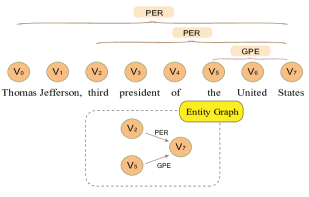
Figure 1: An example of nested named entity mentions. Solid lines connect the starting and ending indices of inner nested entities.

Named entity recognition (NER) aims to identify words or phrases that contain the names of pre-defined categories like location, organization or medical codes. Nested NER further deals with entities that can be nested with each other, such as the United States and third president of the United States shown in Figure 1, such phenomenon is quite common in natural language processing (NLP).

NER is commonly regarded as a sequence labeling task Lample et al. (2016); Ma and Hovy (2016); Peters et al. (2017). These approaches only work for non-nested entities (or flat entities), but neglect nested entities. There have been efforts to deal with the nested structure. Ju et al. 2018 introduced a layered sequence labeling model to first recognize innermost entities, and then feed them into the next layer to extract outer entities. However, this model suffers from obvious error propagation. The wrong entities extracted by the previous layer will affect the performance of the next layer. Also, such layered model suffers from the sparsity of entities at high levels. For instance, in the well-known ACE2005 training dataset, there are only two entities in the sixth level. Sohrab and Miwa 2018 proposed a region-based method that enumerates all possible regions and classifies their entity types. However, this model may ignore explicit boundary information. Zheng et al. 2019 combined the layered sequence labeling model and region-based method to locate the entity boundary first, and then utilized the region classification model to predict entities. This model, however, cares less interaction among entities located in outer and inner layers.

In this paper, we propose a bipartite flat-graph network (BiFlaG) for nested NER, which models a nested structure containing arbitrary many layers into two parts: outermost entities and inner entities in all remaining layers. For example, as shown in Figure 1, the outermost entity Thomas Jefferson, third president of the United States is considered as a flat (non-nested) entity, while third president of the United States (in the second layer) and the United States (in the third layer) are taken as inner entities. The outermost entities with the maximum coverage are usually identified in the flat NER module, which commonly adopts a sequence labeling model. All the inner entities are extracted through the graph module, which iteratively propagates information between the start and end nodes of a span using graph convolutional network (GCN) Kipf and Welling (2017). The benefits of our model are twofold: (1) Different from layered models such as Ju et al. (2018), which suffers from the constraints of one-way propagation of information from lower to higher layers, our model fully captures the interaction between outermost and inner layers in a bidirectional way. Entities extracted from the flat module are used to construct entity graph for the graph module. Then, new representations learned from graph module are fed back to the flat module to improve outermost entity predictions. Also, merging all the entities located in inner layers into a graph module can effectively alleviate the sparsity of entities in high levels. (2) Compared with region-based models Sohrab and Miwa (2018); Zheng et al. (2019), our model makes full use of the sequence information of outermost entities, which take a large proportion in the corpus.

The main contributions of this paper can be summarized as follows:

• We introduce a novel bipartite flat-graph network named BiFlaG for nested NER, which incorporates a flat module for outermost entities and a graph module for inner entities.

• Our BiFlaG fully utilizes the sequence information of outermost entities and meanwhile bidirectionally considers the interaction between outermost and inner layers, other than unidirectional delivery of information.

• With extensive experiments on three benchmark datasets (ACE2005, GENIA, and KBP2017), our model outperforms previous state-of-the-art models under the same settings.

2 Model

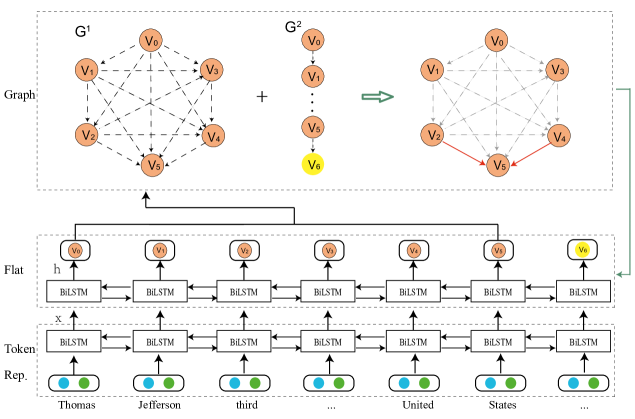
Figure 2: The framework of our BiFlaG model. $G^{1}$ and $G^{2}$ are entity graph and adjacent graph created for GCN, each dashed line connects the start and end nodes for a potential entity. Solid red lines indicate inner entities recognized by the graph module.

Our BiFlaG includes two subgraph modules, a flat NER module and a graph module to learn outermost and inner entities, respectively. Figure 2 illustrates the overview of our model. For the flat module, we adopt BiLSTM-CRF to extract flat (outermost) entities, and use them to construct the entity graph $G^{1}$ as in Figure 2. For the graph module, we use GCN which iteratively propagates information between the start and end nodes of potential entities to learn inner entities. Finally, the learned representation from the graph module is further fed back to the flat module for better outermost predictions.

2.1 Token Representation

Given a sequence consisting of $N$ tokens $\{t_{1},t_{2},...,t_{N}\}$, for each token $t_{i}$, we first concatenate the word-level and character-level embedding $t_{i}=[w_{i};c_{i}$], $w_{i}$ is the pre-trained word embedding, character embedding $c_{i}$ is learned following the work of Xin et al. (2018). Then we use a BiLSTM to capture sequential information for each token $x_{i}=\textsc{BiLSTM}(t_{i})$. We take $x_{i}$ as the word representation and feed it to subsequent modules.

2.2 Flat NER Module

We adopt BiLSTM-CRF architecture Lample et al. (2016); Ma and Hovy (2016); Yang and Zhang (2018); Luo et al. (2020) in our flat module to recognize flat entities, which consists of a bidirectional LSTM (BiLSTM) encoder and a conditional random field (CRF) decoder.

BiLSTM captures bidirectional contextual information of sequences and can effectively represent the hidden states of words in context. BiLSTM represents the sequential information at each step, the hidden state $h$ of BiLSTM can be expressed as follows.

$$\overrightarrow{h_{i}} =LSTM(x_{i},\overrightarrow{h}_{i-1};\overrightarrow{\theta})$$ (1)

$$\overleftarrow{h_{i}} =LSTM(x_{i},\overleftarrow{h}_{i-1};\overleftarrow{\theta})$$

$$h_{i} =[\overrightarrow{h_{i}};\overleftarrow{h_{i}}]$$

where $\overrightarrow{\theta}$ and $\overleftarrow{\theta}$ are trainable parameters. $\overrightarrow{h_{i}}$ and $\overleftarrow{h_{i}}$ respectively denote the forward and backward context representations of token $t_{i}$. The output of BiLSTM $H=\{h_{1},h_{2},...,h_{N}\}$ is further fed into the CRF layer.

CRF Lafferty et al. (2001) has been widely used in state-of-the-art NER models Lample et al. (2016); Ma and Hovy (2016); Yang and Zhang (2018) to help make better decisions, which considers strong label dependencies by adding transition scores between neighboring labels. Viterbi algorithm is applied to search for the label sequence with highest probability during the decoding process. For $y=\{y_{1},...,y_{N}\}$ being a sequence of predictions with length $N$. Its score is defined as follows.

$$s(x,y)=\sum_{i=0}^{N-1}T_{y_{i},y_{i+1}}+\sum_{i=1}^{N}P_{i,y_{i}}$$ (2)

where $T_{y_{i},y_{i+1}}$ represents the transmission score from $y_{i}$ to $y_{i+1}$, $P_{i,y_{i}}$ is the score of the $j^{th}$ tag of the $i^{th}$ word from BiLSTM encoder.

CRF model defines a family of conditional probability $p(y|x)$ over all possible tag sequences $y$:

$$p(y|x)=\frac{\exp^{s(x,y)}}{\sum_{\tilde{y}\in y}\exp^{s(x,\tilde{y})}}$$ (3)

during training phase, we consider the maximum log probability of the correct predictions. While decoding, we search the tag sequences with maximum score:

$$y^{*}=\arg\max_{\tilde{y}\in y}score(x,\tilde{y})$$ (4)

2.3 Graph Module

Since the original input sentences are plain texts without inherent graphical structure, we first construct graphs based on the sequential information of texts and the entity information from the flat module. Then, we apply GCN Kipf and Welling (2017); Qian et al. (2019) which propagates information between neighboring nodes in the graphs, to extract the inner entities.

Graph Construction. We create two types of graphs for each sentence as in Figure 2. Each graph is defined as $G=(V,E)$, where $V$ is the set of nodes (words), $E$ is the set of edges.

• Entity graph $G^{1}$: for all the nodes in an extracted entity extracted from the flat module, edges are added between any two nodes $e_{ij}=(v_{i},v_{j})$, where $start\leq i<j\leq end$, as shown in Figure 2, allowing the outermost entity information to be utilized.

• Adjacent graph $G^{2}$: for each pair of adjacent words in the sentence, we add one directed edge from the left word to the right one, allowing local contextual information to be utilized.

Bi-GCN. In order to consider both incoming and outgoing features for each node, we follow the work of Marcheggiani and Titov (2017); Fu et al. (2019), which uses Bi-GCN to extract graph features. Given a graph $G=(V,E)$, and the word representation $X=\{x_{1},x_{2},...,x_{N}\}$, the graph feature $f\in\mathbb{R}^{N\times d_{f}}$ learned from Bi-GCN is expressed as follows.

$$\overrightarrow{f_{i}} =ReLU(\sum_{{e_{ij}}\in E}(\overrightarrow{W_{f}}x_{j}+\overrightarrow{b_{f}}))$$ (5)

$$\overleftarrow{f_{i}} =ReLU(\sum_{{e_{ji}}\in E}(\overleftarrow{W_{f}}x_{j}+\overleftarrow{b_{f}}))$$

$$f_{i} =[\overrightarrow{f_{i}};\overleftarrow{f_{i}}]$$

where $W_{f}\in\mathbb{R}^{d_{x}\times d_{f}}$ and $b_{f}\in\mathbb{R}^{d_{f}}$ are trainable parameters, $d_{x}$ represents the dimension of word representation, $d_{f}$ is the hidden size of GCN, $ReLU$ is the non-linear activation function. ${e_{ij}}$ represents the edge outgoing from token $t_{i}$, and ${e_{ji}}$ represents the edge incoming to token $t_{i}$.

The features of the two graphs are aggregated to get impacts of both graphs

$$f=W_{c}(f^{1}\oplus f^{2})+b_{c}$$ (6)

where $W_{c}\in\mathbb{R}^{2d_{f}\times d_{f}}$ is the weight to be learned, $b_{c}\in\mathbb{R}^{d_{f}}$ is a bias parameter. $f^{1}$ and $f^{2}$ are graph features of $G^{1}$ and $G^{2}$, respectively.

After getting the graph representation $F=\{f_{1},f_{2},...,f_{N}\}$ from Bi-GCN, we learn the entity score $M\in\mathbb{R}^{N\times N\times L}$ for inner layers as

$$M_{ij}=softmax(W_{3}ReLU(W_{1}f_{i}\oplus W_{2}f_{j}))$$ (7)

where $W_{1},W_{2}\in\mathbb{R}^{d_{f}\times{d_{f}}/2}$, $W_{3}\in\mathbb{R}^{d_{f}\times L}$, $L$ is the number of entity types. $M_{ij}\in\mathbb{R}^{L}$ represents the type probability for a span starts from token $t_{i}$ and ends at token $t_{j}$.

For inner entities, we define the ground truth entity of word pair $(t_{i},t_{j})$ as $\hat{M}_{ij}$, where $t_{i}$ and $t_{j}$ are start and end nodes of a span. Cross Entropy (CE) is used to calculate the loss

$$L_{inner}= -(\sum(\hat{M}_{ij}\text{log}(M_{ij}))\cdot I(\rm O)+$$ (8)

$$\lambda_{1}\cdot\sum(\hat{M}_{ij}\text{log}(M_{ij}))\cdot(1-I(\rm O)))$$

where $M_{ij}\in\mathbb{R}^{L}$ denotes the entity score in the graph module. $I(\rm O)$ is a switching function to distinguish the loss of non-entity ’O’ and other entity types. It is defined as follows.

$$I(\rm O)=\left\{\begin{aligned} 1,\text{if type $=$ '\rm O'}\\ 0,\text{if type $\neq$ '\rm O'}\end{aligned}\right.$$ (9)

$\lambda_{1}$ is the bias weight. The larger $\lambda_{1}$ is, the greater impacts of entity types, and the smaller influences of non-entity ’O’ on the graph module.

Algorithm 1 Bipartite Flat-Graph Algorithm

1:word representations $X=\{x_{1},..,x_{N}\}$,
number of entity types $L$
the dimension of word embeddings $d_{x}$,
the hidden size of GCN $d_{f}$

2:all the entities in this sequence

3:for numbers of training iterations do

4:     $y\leftarrow$ BiLSTM-CRF($X$)

5:     create entity graph $G^{1}$ based on $y$

6:     $F_{N\times d_{f}}\leftarrow$ Bi-GCN($X,G^{1}$)

7:     $M_{N\times N\times L}\leftarrow$ Linear($F\times F$)

8:     transform $M$ to graph $G^{3}$ by Eq.(10)

9:     $X^{new}\leftarrow$ Bi-GCN($X,G^{3}$)

10:     $y^{new}\leftarrow$ BiLSTM-CRF($X^{new}$)

11:     entity set $T$ $\leftarrow$ entities in $M$ and $y^{new}$

12:end for

13:return entity set $T$

	ACE2005						GENIA
	Train	(%)	Dev	(%)	Test	(%)	Train	(%)	Dev	(%)	Test	(%)
# sentences	7,285		968		1,058		15,022		1,669		1,854
with o.l.	2,820	(39)	356	(37)	344	(33)	3,432	(23)	384	(23)	467	(25)
# mentions	24,827		3,234		3,028		47,027		4,469		5,596
outermost entity	18,656	(75)	2,501	(77)	2,313	(76)	42,558	(90)	4,030	(90)	4,958	(89)
inner entity	6,171	(25)	733	(23)	715	(24)	4,469	(10)	439	(10)	642	(11)

Table 1: Statistics of the datasets used in our experiments: ACE2005 and KBP2017. o.l.: overlapping mentions.

2.4 BiFlaG Training

The entity score $M$ in Eq.(7) carries the type probability of each word pair in the sentence. To further consider the information propagation from inner entities to outer ones, we use Bi-GCN to generate new representations from entity score $M$ for the flat module. The largest type score $r_{ij}$ of the word pair $(t_{i},t_{j})$ indicates whether this span is an entity or non-entity and the confidence score of being such type, which is obtained by a max-pooling operation:

$$r_{ij}=\left\{\begin{aligned} max(m_{ij}),\text{if type $\neq$ 'O'}\\ 0,\text{if type $=$ 'O'}\end{aligned}\right.$$ (10)

where type represents the entity type or non-entity ’O’ corresponding to the maximum type score. When the corresponding type is O, there exits no dependencies between $t_{i}$ and $t_{j}$, thus we set $r_{ij}$ to 0. A new graph that carries the boundary information of inner entities is defined as $G^{3}=(V,E)$, where $r_{ij}\in E$.

The new representation used to update flat module consists of two parts. The first part carries the previous representation of each token

$$\alpha_{i}^{1}=W_{r}x_{i}+b_{r}$$ (11)

where $W_{r}\in\mathbb{R}^{d_{x}\times d_{f}}$, $b_{r}\in\mathbb{R}^{d_{f}}$. The second part aggregates inner entity dependencies of the new graph $G^{3}$

$$\alpha_{i}^{2}=\textsc{Bi-GCN}(x_{i},G^{3})$$ (12)

Finally, $\alpha_{i}^{1}$ and $\alpha_{i}^{2}$ are added to obtain the new representation

$$x_{i}^{new}=\alpha_{i}^{1}+\alpha_{i}^{2}$$ (13)

$x_{i}^{new}$ is fed into the flat module to update the parameters and extract better outermost entities.

For outermost entities, we use the BIOES sequence labeling scheme and adopt CRF to calculate the loss. The losses corresponding to the two representations ($X$ and $X^{new}$) are added together as the outermost loss

$$L_{outer}=CRF_{X}+CRF_{X^{new}}$$ (14)

Entities in the sequence are divided into two disjoint sets of outermost and inner entities, which are modeled by flat module and graph module, respectively. Entities in each module share the same neural network structure. Between two modules, each entity in the flat module is either an independent node, or interacting with one or more entities in the graph module. Therefore, Our BiFlaG is indeed a bipartite graph. Our complete training procedure for BiFlaG is shown in Algorithm 1.

2.5 Loss Function

Our BiFlaG model predicts both outermost and inner entities. The total loss is defined as

$$L=L_{outer}+\lambda_{2}L_{inner}$$ (15)

where $\lambda_{2}$ is a weight between loss of flat module and graph module. We minimize this total loss during training phase.

	ACE2005			GENIA			KBP2017
Model	P	R	F1	P	R	F1	P	R	F1
LSTM-CRF Lample et al. (2016)	70.3	55.7	62.2	75.2	64.6	69.5	71.5	53.3	61.1
Multi-CRF	69.7	61.3	65.2	73.1	64.9	68.8	69.7	60.8	64.9
layered-CRF Ju et al. (2018)	74.2	70.3	72.2	78.5	71.3	74.7	-	-	-
LSTM. hyp Katiyar and Cardie (2018)	70.6	70.4	70.5	79.8	68.2	73.6	-	-	-
Segm. hyp [POS] Wang and Lu (2018)	76.8	72.3	74.5	77.0	73.3	75.1∗	79.2	66.5	72.3
Exhaustive Sohrab and Miwa (2018)	-	-	-	73.3	68.3	70.7	-	-	-
Anchor-Region [POS] Lin et al. (2019a)	76.2	73.6	74.9	75.8	73.9	74.8	77.7	71.8	74.6∗
Merge & Label Fisher and Vlachos (2019)	75.1	74.1	74.6†	-	-	-	-	-	-
Boundary-aware Zheng et al. (2019)	-	-	-	75.9	73.6	74.7†	-	-	-
GEANN [Gazetter] Lin et al. (2019b)	77.1	73.3	75.2∗	-	-	-	-	-	-
KBP2017 Overview Ji et al. (2017)	-	-	-	-	-	-	72.6	73.0	72.8†
BiFlaG	75.0	75.2	75.1	77.4	74.6	76.0	77.1	74.3	75.6
			(-0.1∗)			(+0.9∗)			(+1.0∗)

Table 2: Experimental results on ACE2005, GENIA and KBP2017 datasets. POS and Gazetteer indicates using additional POS tags and gazetteers. ^† represents previous state-of-the-art results under the same settings with our experiments, ^∗ represents state-of-the-art results with POS tags or gazetteers, values in parentheses are also compared with them.

3 Experiment

3.1 Dataset and Metric

We evaluate our BiFlaG on three standard nested NER datasets: GENIA, ACE2005, and TACKBP2017 (KBP2017) datasets, which contain 22%, 10% and 19% nested mentions, respectively. Table 1 lists the concerned data statistics.

GENIA dataset Kim et al. (2003) is based on the GENIAcorpus3.02p. We use the same setup as previous works Finkel and Manning (2009); Lu and Roth (2015); Lin et al. (2019a). This dataset contains 5 entity categories and is split into 8.1:0.9:1 for training, development and test.

ACE2005 Walker et al. (2006) contains 7 fine-grained entity categories. We preprocess the dataset following the same settings of Lu and Roth (2015); Wang and Lu (2018); Katiyar and Cardie (2018); Lin et al. (2019a) by keeping files from bn, nw and wl, and splitting these files into training, development and test sets by 8:1:1, respectively.

KBP2017 Following Lin et al. (2019a), we evaluate our model on the 2017 English evaluation dataset (LDC2017E55). The training and development sets contain previous RichERE annotated datasets (LDC2015E29, LDC2015E68, LDC2016E31 and LDC2017E02). The datasets are split into 866/20/167 documents for training, development and test, respectively.

Metric Precision ($P$), recall ($R$) and F-score ($F_{1}$) are used to evaluate the predicted entities. An entity is confirmed correct if it exists in the target labels, regardless of the layer at which the model makes this prediction.

3.2 Parameter Settings

Our model is based on the framework of Yang and Zhang (2018). We conduct optimization with the stochastic gradient descent (SGD) and Adam for flat and GCN modules, respectively. For GENIA dataset, we use the same 200-dimension pre-trained word embedding as Ju et al. (2018); Sohrab and Miwa (2018); Zheng et al. (2019). For ACE2005 and KBP2017 datasets, we use the publicly available pre-trained 100-dimension GloVe Pennington et al. (2014) embedding. We train the character embedding as in Xin et al. (2018). The learning rate is set to 0.015 and 0.001 for flat and GCN modules, respectively. We apply dropout to embeddings and the hidden states with a rate of 0.5. The hidden sizes of BiLSTM and GCN are both set to 256. The bias weights $\lambda_{1}$ and $\lambda_{2}$ are both set to 1.5.

3.3 Results and Comparisons

Table 5 compares our model to some existing state-of-the-art approaches on the three benchmark datasets. Given only standard training data and publicly available word embeddings, the results in Table 2 show that our model outperforms all these models. Current state-of-the-art results on these datasets are tagged with ^† in Table 5, we make improvements of 0.5/1.3/2.8 $F_{1}$ on ACE2005, GENIA, and KBP2017 respectively. KBP2017 contains much more entities than ACE2005 and GENIA. The number of entities on test set is four times that of ACE2005. Our model has the most significant improvement on such dataset, proving the effectiveness of our BiFlaG model. More notably, our model without POS tags surpasses the previous models Wang and Lu (2018); Lin et al. (2019a), which use POS tags as additional representations on all three datasets. Besides, Lin et al. (2019b) incorporate gazetteer information on ACE2005 dataset, our model also makes comparable results with theirs. Other works like Straková et al. (2019) , which train their model on both training and development sets, are thus not comparable to our model directly.

	Our model				Boundary-aware				Layered-CRF
Category	P	R	F		P	R	F		P	R	F		Num.
DNA	72.7	72.7	72.7		73.6	67.8	70.6		74.4	69.7	72.0		1,290
RNA	84.4	84.4	84.4		82.2	80.7	81.5		90.3	79.5	84.5		117
Protein	79.5	76.5	78.0		76.7	76.0	76.4		80.5	73.2	76.7		3,108
Cell Line	75.9	67.6	71.5		77.8	65.8	71.3		77.8	65.7	71.2		462
Cell Type	76.7	72.4	74.4		73.9	71.2	72.5		76.4	68.1	72.0		619
Overall	77.4	74.6	76.0		75.8	73.6	74.7		78.5	71.3	74.7		5,596

Table 3: Our results on five categories compared to Zheng et al. (2019) and Ju et al. (2018) on GENIA dataset.

Table 3 makes a detailed comparison on the five categories of GENIA test dataset with a layered model Ju et al. (2018) and a region-based model Zheng et al. (2019). Compared with region-based model, layered model seems to have higher precision and lower recall, for they are subject to error propagate, the outer entities will not be identified if the inner ones are missed. Meanwhile, region-based model suffers from low precision, as they may generate a lot of candidate spans. By contrast, our BiFlaG model well coordinates precision and recall. The entity types Protein and DNA have the most nested entities on GENIA dataset, the improvement of our BiFlaG on these two entity types is remarkable, which can be attributed to the interaction of nested information between the two subgraph modules of our BiFlaG.

3.4 Analysis of Each Module

Table 4 evaluates the performance of each module on ACE2005 and GENIA datasets. Our flat module performs well on both datasets for outermost entity recognition. However, the recall of the inner entities is low on GENIA dataset. According to the statistics in Table 1, only 11% of the entities on GENIA are located in inner layers, while on ACE2005 dataset, the proportion is 24%. It can be inferred that the sparsity of the entity distribution in inner layers has a great impact on the results. If these inner entities are identified at each layer, the sparsity may be even worse. We can enhance the impact of sparse entities by increasing the weight $\lambda_{1}$ in Eq.(14), but this may hurt precision, we set $\lambda_{1}=1.5$ to have a better tradeoff between precision and recall.

	ACE2005			GENIA
	P	R	F	P	R	F
Outermost	73.7	75.0	74.3	78.4	78.9	78.7
Inner	58.3	55.2	56.7	50.9	34.7	41.2

Table 4: Performance of each module on ACE2005 and GENIA datasets.

	ACE2005	GENIA	KBP2017
Flat $\rightarrow$ Grpah
no graph	73.4	74.4	74.0
adjacent graph	73.8	74.9	74.7
entity graph	74.8	75.5	75.2
both graphs	75.1	76.0	75.6
Graph $\rightarrow$ Flat
without	74.3	74.5	75.1
with	75.1	76.0	75.6

Table 5: Ablation study on the three benchmark datasets.

3.5 Analysis of Entity Length

We conduct additional experiments on ACE2005 dataset to detect the effect of the lengths of the outermost entities on the extraction of their inner entities as shown in Table 6. Our flat module can well predict outermost entities which account for a large proportion among all types of entities. In general, the performance of inner entities is affected by the extracting performance and length of their outermost entities. A shorter outermost entity is more likely to have its inner entities shared either the first token or the last token, making the constructed graph more instructive, thus its inner entities are easier to extract.

length		outermost entities					inner entities
		P	R	F	Num.		P	R	F	Num.
1		75.9	80.6	78.2	1,260		-	-	-	-
2		72.1	74.8	73.4	488		76.6	63.6	69.5	77
3		67.8	72.2	69.9	198		67.6	56.5	61.5	85
4		62.5	60.9	61.7	112		68.1	42.3	52.2	111
5		60.7	48.7	54.0	76		56.0	37.8	45.1	74
6		46.3	46.3	46.3	41		28.0	25.9	26.9	54
7		44.4	30.8	36.4	26		21.7	16.7	18.9	30
8		64.3	40.9	50.0	22		31.8	21.2	25.5	33
9		35.7	31.3	33.3	16		23.1	19.4	21.1	31
10		57.1	22.2	32.0	18		20.0	15.4	17.4	26

Table 6: Length-wise results on ACE2005 test dataset.

3.6 Ablation Study

In this paper, we use the interactions of flat module and graph module to respectively help better predict outermost and inner entities. We conduct ablation study to verify the effectiveness of the interactions. The first part is the information delivery from the flat module to the graph module. We conduct four experiments: (1) no graph: we skip Eq. (5)-(6) and let graph feature $f=\textsc{Linear}(x)$. In this case, inner entities are independent of the outermost entities and only rely on the word representation (section 2.1) which carries contextualized information. (2) adjacent graph: we further utilize the sequential information of the text to help inner entity prediction. (3) entity graph: the boundary information of outer entities can be indicative for inner entities, we construct an entity graph based on the entities extracted by the flat module. (4) both graphs: when outer entities are not recognized by the flat module, their inner entities will fail to receive the boundary information, we use the sequential information of the text to make up for the deficiency of using only entity graph. Experimental results show that entity graph carries more useful information than adjacent graph, which enhances the baseline by 1.4/1.1/1.2 $F_{1}$ score, respectively. By combing these two graphs together, we get a larger gain of 1.7/1.6/1.6 $F_{1}$ score. The second part is the information delivery from the graph module to the flat module, the new representation $X^{new}$ learned from graph module is propagated back to the flat module. $X^{new}$ is equipped with the dependencies of inner entities and shows useful, yielding an improvement of 0.8/1.5/0.5 $F_{1}$ for the three benchmarks, respectively.

3.7 Inference Time

We examine the inference speed of our BiFlaG with Zheng et al. (2019), Sohrab and Miwa (2018) and Ju et al. (2018) in terms of the number of words decoded per second. For all the compared models, we use the re-implemented code released by Zheng et al. (2019) and set the same batch size 10. Compared with Zheng et al. (2019) and Sohrab and Miwa (2018), our BiFlaG does not need to compute region representation for each potential entity, thus we can take full advantage of GPU parallelism. Compared with Ju et al. (2018), which requires CRF decoding for each layer, our model only needs to calculate two modules, by contrast, the cascaded CRF layers limit their inference speed.

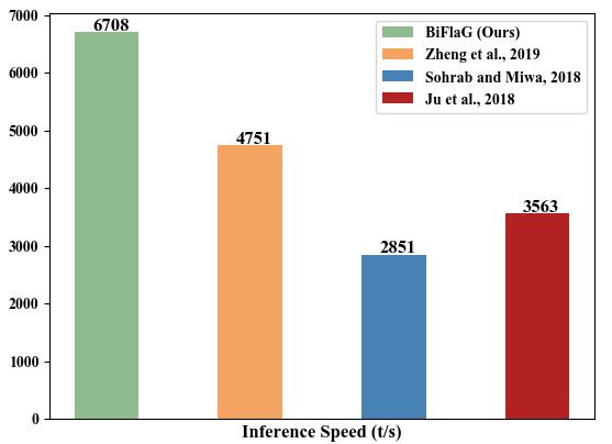
Figure 3: The inference speed of our BiFlaG and compared models on GENIA test set. t/s indicates token per second.

Setence	Interesting aside: Starbucks is taking over the location in my town that was recently abandoned by Krispy Kreme.
Gold Label	ORG: {Starbucks, Krispy Kreme}; FAC: {the location in my town that was recently abandoned by Krispy Kreme; that}; GPE: {my town}; PER: {my}
No Graph	ORG: {Starbucks}; LOC: {the location in my town that was recently abandoned by Krispy Kreme}; PER: {my}
No interaction	ORG: {Starbucks, Krispy Kreme}; LOC: {the location in my town that was recently abandoned by Krispy Kreme}; GPE: {my town}; PER: {my}
BiFlaG	ORG: {Starbucks, Krispy Kreme }; FAC: {the location in my town that was recently abandoned by Krispy Kreme; that}; GPE: {my town}; PER: {my}

Table 7: An example of predicted results in ACE2005 test dataset.

4 Case Study

Table 7 shows a case study of each module in our model. In this example, entities my, my town, that and Krispy Kreme are nested in the entity the location in my town that was recently abandoned by Krispy Kreme. Our BiFlaG model successfully extracts all these entities with exact boundaries and entity categorical labels. Without graph construction, nested entities my town, that and Krispy Kreme are not identified. Without interaction between the two modules, the outermost entity the location in my town that was recently abandoned by Krispy Kreme is mislabeled as LOC (location), which is actually a FAC (Facility) type, inner nested entities my, my town and Krispy Kreme are not propagated back to the flat module, which maybe helpful to correct the extracting of the outermost entity.

5 Related Work

Recently, with the development of deep neural network in a wide range of NLP tasks Bai and Zhao (2018); Huang et al. (2018); Huang and Zhao (2018); He et al. (2018, 2019); Li et al. (2018a, b, 2019); Zhou and Zhao (2019); Xiao et al. (2019); Zhang and Zhao (2018); Zhang et al. (2019, 2020a, 2020b, 2020c), it is possible to build reliable NER systems without hand-crafted features. Nested named entity recognition requires to identity all the entities in texts that may be nested with each other. Though NER is a traditional NLP task, it is not until the very recent years that researches have been paid to this nested structure for named entities.

Lu and Roth (2015) introduce a novel hypergraph representation to handle overlapping mentions. Muis and Lu (2017) further develop a gap-based tagging schema that assigns tags to gaps between words to address the spurious structures issue, which can be modeled using conventional linear-chain CRFs. However, it suffers from the structural ambiguity issue during inference. Wang and Lu (2018) propose a novel segmental hypergraph representation to eliminate structural ambiguity. Katiyar and Cardie (2018) also propose a hypergraph-based approach based on the BILOU tag scheme that utilizes an LSTM network to learn the hypergraph representation in a greedy manner.

Stacking sequence labeling models to extract entities from inner to outer (or outside-to-inside) can also handle such nested structures. Alex et al. (2007) propose several different modeling techniques (layering and cascading) to combine multiple CRFs for nested NER. However, their approach cannot handle nested entities of the same entity type. Ju et al. (2018) dynamically stack flat NER layers, and recognize entities from innermost layer to outer ones. Their approach can deal with nested entities of the same type, but suffers from error propagation among layers.

Region-based approaches are also commonly used for nested NER by extracting the subsequences in sentences and classifying their types. Sohrab and Miwa (2018) introduce a neural exhaustive model that considers all possible spans and classify their types. This work is further improved by Zheng et al. (2019), which first apply a single-layer sequence labeling model to identify the boundaries of potential entities using context information, and then classify these boundary-aware regions into their entity type or non-entity. Lin et al. (2019a) propose a sequence-to-nuggets approach named as Anchor-Region Networks (ARNs) to detect nested entity mentions. They first use an anchor detector to detect the anchor words of entity mentions and then apply a region recognizer to identity the mention boundaries centering at each anchor word. Fisher and Vlachos (2019) decompose nested NER into two stages. Tokens are merged into entities through real-valued decisions, and then the entity embeddings are used to label the entities identified.

6 Conclusion

This paper proposes a new bipartite flat-graph (BiFlaG) model for nested NER which consists of two interacting subgraph modules. Applying the divide-and-conquer policy, the flat module is in charge of outermost entities, while the graph module focuses on inner entities. Our BiFlaG model also facilitates a full bidirectional interaction between the two modules, which let the nested NE structures jointly learned at most degree. As a general model, our BiFlaG model can also handle non-nested structures by simply removing the graph module. In terms of the same strict setting, empirical results show that our model generally outperforms previous state-of-the-art models.

References

- Alex et al. (2007) Beatrice Alex, Barry Haddow, and Claire Grover. 2007. Recognising nested named entities in biomedical text. In Biological, translational, and clinical language processing, pages 65–72.
- Bai and Zhao (2018) Hongxiao Bai and Hai Zhao. 2018. Deep enhanced representation for implicit discourse relation recognition. In Proceedings of the 27th International Conference on Computational Linguistics, pages 571–583.
- Finkel and Manning (2009) Jenny Rose Finkel and Christopher D. Manning. 2009. Nested named entity recognition. In Proceedings of the 2009 Conference on Empirical Methods in Natural Language Processing, pages 141–150.
- Fisher and Vlachos (2019) Joseph Fisher and Andreas Vlachos. 2019. Merge and label: A novel neural network architecture for nested NER. In Proceedings of the 57th Annual Meeting of the Association for Computational Linguistics, pages 5840–5850.
- Fu et al. (2019) Tsu-Jui Fu, Peng-Hsuan Li, and Wei-Yun Ma. 2019. GraphRel: Modeling text as relational graphs for joint entity and relation extraction. In Proceedings of the 57th Annual Meeting of the Association for Computational Linguistics, pages 1409–1418.
- He et al. (2019) Shexia He, Zuchao Li, and Hai Zhao. 2019. Syntax-aware multilingual semantic role labeling. In Proceedings of the 2019 Conference on Empirical Methods in Natural Language Processing and the 9th International Joint Conference on Natural Language Processing (EMNLP-IJCNLP), pages 5350–5359.
- He et al. (2018) Shexia He, Zuchao Li, Hai Zhao, and Hongxiao Bai. 2018. Syntax for semantic role labeling, to be, or not to be. In Proceedings of the 56th Annual Meeting of the Association for Computational Linguistics (Volume 1: Long Papers), pages 2061–2071.
- Huang et al. (2018) Yafang Huang, Zuchao Li, Zhuosheng Zhang, and Hai Zhao. 2018. Moon IME: Neural-based Chinese pinyin aided input method with customizable association. In Proceedings of ACL 2018, System Demonstrations, pages 140–145.
- Huang and Zhao (2018) Yafang Huang and Hai Zhao. 2018. Chinese pinyin aided IME, input what you have not keystroked yet. In Proceedings of the 2018 Conference on Empirical Methods in Natural Language Processing, pages 2923–2929.
- Ji et al. (2017) Heng Ji, Xiaoman Pan, Boliang Zhang, Joel Nothman, James Mayfield, Paul McNamee, and Cash Costello. 2017. Overview of tac-kbp2017 13 languages entity discovery and linking. Theory and Applications of Categories.
- Ju et al. (2018) Meizhi Ju, Makoto Miwa, and Sophia Ananiadou. 2018. A neural layered model for nested named entity recognition. In Proceedings of the 2018 Conference of the North American Chapter of the Association for Computational Linguistics: Human Language Technologies, Volume 1 (Long Papers), pages 1446–1459.
- Katiyar and Cardie (2018) Arzoo Katiyar and Claire Cardie. 2018. Nested named entity recognition revisited. In Proceedings of the 2018 Conference of the North American Chapter of the Association for Computational Linguistics: Human Language Technologies, Volume 1 (Long Papers), pages 861–871.
- Kim et al. (2003) J-D Kim, Tomoko Ohta, Yuka Tateisi, and Jun’ichi Tsujii. 2003. Genia corpus—a semantically annotated corpus for bio-textmining. Bioinformatics, pages i180–i182.
- Kipf and Welling (2017) Thomas N Kipf and Max Welling. 2017. Semi-supervised classification with graph convolutional networks. In International Conference on Learning Representations (ICLR).
- Lafferty et al. (2001) John D. Lafferty, Andrew Mccallum, and Fernando C. N. Pereira. 2001. Conditional random fields: Probabilistic models for segmenting and labeling sequence data. In International Conference on Machine Learning.
- Lample et al. (2016) Guillaume Lample, Miguel Ballesteros, Sandeep Subramanian, Kazuya Kawakami, and Chris Dyer. 2016. Neural architectures for named entity recognition. In Proceedings of the 2016 Conference of the North American Chapter of the Association for Computational Linguistics: Human Language Technologies, pages 260–270.
- Li et al. (2018a) Zuchao Li, Jiaxun Cai, Shexia He, and Hai Zhao. 2018a. Seq2seq dependency parsing. In Proceedings of the 27th International Conference on Computational Linguistics, pages 3203–3214.
- Li et al. (2018b) Zuchao Li, Shexia He, Jiaxun Cai, Zhuosheng Zhang, Hai Zhao, Gongshen Liu, Linlin Li, and Luo Si. 2018b. A unified syntax-aware framework for semantic role labeling. In Proceedings of the 2018 Conference on Empirical Methods in Natural Language Processing, pages 2401–2411.
- Li et al. (2019) Zuchao Li, Shexia He, Hai Zhao, Yiqing Zhang, Zhuosheng Zhang, Xi Zhou, and Xiang Zhou. 2019. Dependency or span, end-to-end uniform semantic role labeling. In Proceedings of the AAAI Conference on Artificial Intelligence, volume 33, pages 6730–6737.
- Lin et al. (2019a) Hongyu Lin, Yaojie Lu, Xianpei Han, and Le Sun. 2019a. Sequence-to-nuggets: Nested entity mention detection via anchor-region networks. In Proceedings of the 57th Annual Meeting of the Association for Computational Linguistics, pages 5182–5192.
- Lin et al. (2019b) Hongyu Lin, Yaojie Lu, Xianpei Han, Le Sun, Bin Dong, and Shanshan Jiang. 2019b. Gazetteer-enhanced attentive neural networks for named entity recognition. In Proceedings of the 2019 Conference on Empirical Methods in Natural Language Processing and the 9th International Joint Conference on Natural Language Processing (EMNLP-IJCNLP), pages 6232–6237.
- Lu and Roth (2015) Wei Lu and Dan Roth. 2015. Joint mention extraction and classification with mention hypergraphs. In Proceedings of the 2015 Conference on Empirical Methods in Natural Language Processing, pages 857–867.
- Luo et al. (2020) Ying Luo, Fengshun Xiao, and Hai Zhao. 2020. Hierarchical contextualized representation for named entity recognition. In the Thirty-Fourth AAAI Conference on Artificial Intelligence (AAAI-2020).
- Ma and Hovy (2016) Xuezhe Ma and Eduard Hovy. 2016. End-to-end sequence labeling via bi-directional LSTM-CNNs-CRF. In Proceedings of the 54th Annual Meeting of the Association for Computational Linguistics (Volume 1: Long Papers), pages 1064–1074.
- Marcheggiani and Titov (2017) Diego Marcheggiani and Ivan Titov. 2017. Encoding sentences with graph convolutional networks for semantic role labeling. In Proceedings of the 2017 Conference on Empirical Methods in Natural Language Processing, pages 1506–1515.
- Muis and Lu (2017) Aldrian Obaja Muis and Wei Lu. 2017. Labeling gaps between words: Recognizing overlapping mentions with mention separators. In Proceedings of the 2017 Conference on Empirical Methods in Natural Language Processing, pages 2608–2618. Association for Computational Linguistics.
- Pennington et al. (2014) Jeffrey Pennington, Richard Socher, and Christopher Manning. 2014. Glove: Global vectors for word representation. In Proceedings of the 2014 Conference on Empirical Methods in Natural Language Processing (EMNLP), pages 1532–1543.
- Peters et al. (2017) Matthew Peters, Waleed Ammar, Chandra Bhagavatula, and Russell Power. 2017. Semi-supervised sequence tagging with bidirectional language models. In Proceedings of the 55th Annual Meeting of the Association for Computational Linguistics (Volume 1: Long Papers), pages 1756–1765.
- Qian et al. (2019) Yujie Qian, Enrico Santus, Zhijing Jin, Jiang Guo, and Regina Barzilay. 2019. GraphIE: A graph-based framework for information extraction. In Proceedings of the 2019 Conference of the North American Chapter of the Association for Computational Linguistics: Human Language Technologies, Volume 1 (Long and Short Papers), pages 751–761.
- Sohrab and Miwa (2018) Mohammad Golam Sohrab and Makoto Miwa. 2018. Deep exhaustive model for nested named entity recognition. In Proceedings of the 2018 Conference on Empirical Methods in Natural Language Processing, pages 2843–2849.
- Straková et al. (2019) Jana Straková, Milan Straka, and Jan Hajic. 2019. Neural architectures for nested NER through linearization. In Proceedings of the 57th Annual Meeting of the Association for Computational Linguistics, pages 5326–5331.
- Walker et al. (2006) Christopher Walker, Stephanie Strassel, Julie Medero, and Kazuaki Maeda. 2006. Ace 2005 multilingual training corpus. Linguistic Data Consortium, Philadelphia, 57.
- Wang and Lu (2018) Bailin Wang and Wei Lu. 2018. Neural segmental hypergraphs for overlapping mention recognition. In Proceedings of the 2018 Conference on Empirical Methods in Natural Language Processing, pages 204–214.
- Xiao et al. (2019) Fengshun Xiao, Jiangtong Li, Hai Zhao, Rui Wang, and Kehai Chen. 2019. Lattice-based transformer encoder for neural machine translation. In Proceedings of the 57th Annual Meeting of the Association for Computational Linguistics, pages 3090–3097.
- Xin et al. (2018) Yingwei Xin, Ethan Hart, Vibhuti Mahajan, and Jean-David Ruvini. 2018. Learning better internal structure of words for sequence labeling. In Proceedings of the 2018 Conference on Empirical Methods in Natural Language Processing, pages 2584–2593.
- Yang and Zhang (2018) Jie Yang and Yue Zhang. 2018. NCRF++: An open-source neural sequence labeling toolkit. In Proceedings of ACL 2018, System Demonstrations, pages 74–79.
- Zhang et al. (2020a) Shuailiang Zhang, Hai Zhao, Yuwei Wu, Zhuosheng Zhang, Xi Zhou, and Xiang Zhou. 2020a. DCMN+: Dual co-matching network for multi-choice reading comprehension. In the Thirty-Fourth AAAI Conference on Artificial Intelligence (AAAI-2020).
- Zhang et al. (2019) Zhuosheng Zhang, Yafang Huang, and Hai Zhao. 2019. Open vocabulary learning for neural Chinese pinyin IME. In Proceedings of the 57th Annual Meeting of the Association for Computational Linguistics, pages 1584–1594.
- Zhang et al. (2020b) Zhuosheng Zhang, Yuwei Wu, Hai Zhao, Zuchao Li, Shuailiang Zhang, Xi Zhou, and Xiang Zhou. 2020b. Semantics-aware BERT for language understanding. In the Thirty-Fourth AAAI Conference on Artificial Intelligence (AAAI-2020).
- Zhang et al. (2020c) Zhuosheng Zhang, Yuwei Wu, Junru Zhou, Sufeng Duan, and Hai Zhao. 2020c. SG-Net: Syntax-guided machine reading comprehension. In the Thirty-Fourth AAAI Conference on Artificial Intelligence (AAAI-2020).
- Zhang and Zhao (2018) Zhuosheng Zhang and Hai Zhao. 2018. One-shot learning for question-answering in Gaokao history challenge. In Proceedings of the 27th International Conference on Computational Linguistics, pages 449–461.
- Zheng et al. (2019) Changmeng Zheng, Yi Cai, Jingyun Xu, Ho-fung Leung, and Guandong Xu. 2019. A boundary-aware neural model for nested named entity recognition. In Proceedings of the 2019 Conference on Empirical Methods in Natural Language Processing and the 9th International Joint Conference on Natural Language Processing (EMNLP-IJCNLP), pages 357–366.
- Zhou and Zhao (2019) Junru Zhou and Hai Zhao. 2019. Head-driven phrase structure grammar parsing on Penn treebank. In Proceedings of the 57th Annual Meeting of the Association for Computational Linguistics, pages 2396–2408.