Time-Scales for Nonlinear Processes in Preheating after Multifield Inflation with Nonminimal Couplings

Abstract

We have conducted extensive lattice simulations to study the post-inflation dynamics of multifield models involving nonminimal couplings. We explore the parameter dependence of preheating in these models and describe the various time-scales that control such nonlinear processes as energy transfer, re-scattering, and the approach to radiation-domination and thermalization. In the limit of large nonminimal couplings ($\xi_{I}\sim 100$), we find that efficient transfer of energy from the inflaton condensate to radiative degrees of freedom, emergence of a radiation-dominated equation of state, and the onset of thermalization each consistently occur within $N_{\rm reh}\lesssim 3$ $e$-folds after the end of inflation, largely independent of the values of the other couplings in the models. The exception is the case of negative ellipticity, in which there is a misalignment between the dominant direction in field-space along which the system evolves and the larger of the nonminimal couplings $\xi_{I}$. In those cases, the field-space-driven parametric resonance is effectively shut off. More generally, the competition between the scalar fields’ potential and the field-space manifold structure can yield interesting phenomena such as two-stage resonances. Across many regions of parameter space, we find efficient re-scattering between the distinct fields, leading to a partial memory loss of the shape of the initial fluctuation spectrum. Despite the explosive particle production, which can lead to a quick depletion of the background energy density, the nonlinear processes do not induce any super-horizon correlations after the end of inflation in these models, which keeps predictions for CMB observables unaffected by the late-time amplification of isocurvature fluctuations. Hence the excellent agreement between primordial observables and recent observations is preserved for this class of models, even when we consider post-inflation dynamics.

I Introduction

Inflation is the leading framework for studying the very early universe, and predictions from several inflationary models are consistent with high-precision cosmological observations, including the Planck measurements of the cosmic microwave background radiation (CMB) and large-scale structure surveys Guth et al. (2014); Martin (2016); Chowdhury et al. (2019). However, calculations of predictions for observables from inflationary models are subject to uncertainty arising from the limited amount of information we have regarding the post-inflation reheating era. Reheating is the period during which the energy density that had been locked in the inflaton condensate is transferred to radiation modes that (will eventually) become the Standard Model and Dark Matter sectors. The expansion of the universe thus transitions from a quasi-de Sitter phase during inflaton to a radiation-dominated phase at the end of reheating. The duration of reheating and corresponding equation of state affect the relation between the times of horizon exit and re-entry for inflationary fluctuations Martin and Ringeval (2010); Mielczarek (2011); Martin et al. (2015); Munoz and Kamionkowski (2015); Creminelli et al. (2014a, b); Dai et al. (2014); Cai et al. (2015); Cook et al. (2015); Eshaghi et al. (2016); Ueno and Yamamoto (2016); Figueroa and Tanin (2019). Reheating is thus a crucial phase to understand, in order to connect the primordial phase of inflation with the conditions required for the onset of standard Big Bang evolution, as well as to refine predictions for observables from inflationary models. Reheating can proceed either through perturbative decays of the inflaton into lighter particles (perturbative reheating), or through nonperturbative processes such as parametric resonance (preheating), which yield an exponential enhancement of radiation modes. The latter process — when efficient enough — can lead to very fast reheating and the emergence of nonlinear effects, such as oscillon formation Amin (2010); Amin et al. (2010); Gleiser et al. (2011); Amin et al. (2012); Lozanov and Amin (2018); Hong et al. (2018); Fukunaga et al. (2019). (For reviews of reheating, see Refs. Bassett et al. (2006); Frolov (2010); Allahverdi et al. (2010); Amin et al. (2014); Lozanov (2019).)

In this work we study a family of models that incorporates realistic features from high-energy physics, namely multiple interacting scalar fields, each coupled nonminimally to the space-time Ricci scalar. Nonminimal couplings of the form $\xi\phi^{2}R$, where $\xi$ is a dimensionless coupling, $\phi$ is a scalar field, and $R$ is the spacetime Ricci scalar, necessarily arise as renormalization counterterms for self-interacting scalar fields in curved spacetime Callan et al. (1970); Bunch et al. (1980); Bunch and Panangaden (1980); Birrell and Davies (1982); Odintsov (1991); Buchbinder et al. (1992); Parker and Toms (2009); Markkanen and Tranberg (2013). Furthermore, the values of nonminimal couplings typically increase with energy scale under renormalization-group flow, with no UV fixed points Odintsov (1991); Buchbinder et al. (1992). We thus expect multiple scalar fields to be present during inflation, each with a potentially large nonminimal coupling. Higgs inflation Bezrukov and Shaposhnikov (2008); Greenwood et al. (2013); Sfakianakis and van de Vis (2019); Ema et al. (2020) is a well-known example from this class of models.

This class of models yields an excellent fit between predictions and CMB observables, when such predictions are calculated based only on the dynamics during inflation Kaiser and Sfakianakis (2014). Yet it is critical to understand the time-scales over which distinct processes during the post-inflation reheating phase unfold, such as the onset of a radiation-dominated equation of state and the emergence of thermal equilibrium at an appropriately high temperature. In this family of models in particular, one must also track the evolution of the single-field attractor Kaiser et al. (2013); Greenwood et al. (2013); Kaiser and Sfakianakis (2014); Schutz et al. (2014) beyond the end of inflation in order to understand whether any post-inflation effects could significantly affect the predictions for primordial observables Nguyen et al. (2019).

As a considerable amount of energy is transferred from the inflaton to radiation modes, the most significant physical processes during (p)reheating are essentially nonlinear. In order to capture non-linear processes during preheating, we conduct large-scale lattice simulations. We consider two-field models, with $\phi^{I}=\{\phi,\chi\}$, and couplings $(\xi_{\phi}\phi^{2}+\xi_{\chi}\chi^{2})R$ in the Lagrangian. We build upon Ref. Nguyen et al. (2019) to identify several distinct nonlinear effects, characteristic of the preheating dynamics, which can unfold on different time-scales. To explore the nonlinear dynamics of this family of models, we focus on several distinct processes and consider how the associated time-scales change as one varies the relevant parameters. We first consider a fairly “generic” set of ratios among the couplings, and study the dynamics of this “benchmark” case across three distinct regimes of $\xi_{\phi}\sim 1,10,100$. We then consider how this behavior shifts for a model that has symmetric couplings as well as for models in which we vary the ellipticity, $\varepsilon\equiv(\xi_{\phi}-\xi_{\chi})/\xi_{\phi}$.

Across these many regions of parameter space, we find a dominant trend that increasing the non-minimal couplings $\xi_{I}$ increases the efficiency of preheating, thereby shortening the time required for energy to be transferred from the inflaton condensate into a (quasi-) thermal bath of produced particles. Throughout parameter space for this family of models, we consistently find the emergence of a radiation-dominated equation of state as well as the onset of thermalization to occur within $N_{\rm reh}\sim{\cal O}(1)$ $e$-folds after the end of inflation. We further find that the single-field attractor that had been identified in previous work Kaiser et al. (2013); Greenwood et al. (2013); Kaiser and Sfakianakis (2014); Schutz et al. (2014) persists through the end of the preheating phase in most cases, thereby protecting the close match between predictions from this family of models and the latest high-precision measurements of CMB observables. Even in the case in which the excitation of the second field is strong enough to break the single-field attractor, this occurs deep into preheating and only after nonlinear effects have rendered the notion of a background trajectory invalid. Furthermore, the average field trajectory does not exhibit super-horizon correlations, and hence cannot affect CMB observables.

In Section II we define the family of models and briefly discuss the behavior of fluctuations, which depend on both the curvature of the field-space manifold and on the topography of the potential. In Section III we examine a characteristic “benchmark” case and define the various time-scales that are relevant for understanding the non-linear dynamics during preheating. In Section III.3 we discuss how the efficiency of preheating and the dynamical time-scales depend on the parameter choices for the potential and field-space manifold. We provide conclusions and discuss future prospects in Section IV.

II Models, Parameters, and Initial Conditions

II.1 Structure of the Models

We study inflationary models consisting of multiple real scalar fields $\phi^{I}$, each nonminimally coupled to the Ricci spacetime curvature scalar. We closely follow the analysis and notation of Refs. Kaiser et al. (2013); Greenwood et al. (2013); Kaiser and Sfakianakis (2014); Schutz et al. (2014); DeCross et al. (2018a, b, c). We work in $(3+1)$ spacetime dimensions and adopt the “mostly plus” spacetime metric signature $(-,+,+,+)$. In the Jordan frame, the action takes the form

$$S=\int d^{4}x\sqrt{-\tilde{g}}\left[f(\phi^{I})\tilde{R}-\frac{1}{2}\delta_{IJ}\tilde{g}^{\mu\nu}\partial_{\mu}\phi^{I}\partial_{\nu}\phi^{J}-\tilde{V}(\phi^{I})\right],$$ (1)

where upper-case Latin letters label field-space indices, $I,J=1,2,...,N$, Greek letters label spacetime indices, $\mu,\nu=0,1,2,3$, and tildes denote Jordan-frame quantities. We will use lower-case Latin letters for spatial indices, $i,j=1,2,3$.

We bring the gravitational portion of the action into canonical Einstein-Hilbert form by performing a conformal transformation, rescaling $\tilde{g}_{\mu\nu}(x)\rightarrow g_{\mu\nu}(x)=\Omega^{2}(x)\>\tilde{g}_{\mu\nu}(x)$ with the function

$$\Omega^{2}(x)=\frac{2}{M_{\rm pl}^{2}}f(\phi^{I}(x)),$$ (2)

where $M_{\rm pl}\equiv 1/\sqrt{8\pi G}=2.43\times 10^{18}$ GeV is the reduced Planck mass. The action in the Einstein frame becomes Kaiser (2010); Abedi and Abbassi (2015)

$$S=\int d^{4}x\sqrt{-g}\left[\frac{M_{\rm pl}^{2}}{2}R-\frac{1}{2}{\cal G}_{IJ}(\phi^{K})g^{\mu\nu}\partial_{\mu}\phi^{I}\partial_{\nu}\phi^{J}-V(\phi^{I})\right]\,,$$ (3)

where the potential is stretched by the conformal factor $f(\phi^{I})$,

$$V(\phi^{I})=\frac{M_{\rm pl}^{4}}{4f^{2}(\phi^{I})}\tilde{V}(\phi^{I}).$$ (4)

In addition, the nonminimal couplings induce a curved field-space manifold in the Einstein frame, with associated field-space metric ${\cal G}_{IJ}(\phi^{K})$

$${\cal G}_{IJ}(\phi^{K})=\frac{M_{\rm pl}^{2}}{2f(\phi^{K})}\left[\delta_{IJ}+\frac{3}{f(\phi^{K})}f_{,I}f_{,J}\right],$$ (5)

where $f_{,I}=\partial f/\partial\phi^{I}$. For multiple fields ($N\geq 2$), one cannot canonically normalize all of the fields while retaining the Einstein-Hilbert form of the gravitational part of the action Kaiser (2010).

Varying the action of Eq. (3) with respect to $g_{\mu\nu}$ yields the field equations

$$R_{\mu\nu}-\frac{1}{2}g_{\mu\nu}R=\frac{1}{M_{\rm pl}^{2}}T_{\mu\nu},$$ (6)

with the energy-momentum tensor given by Kaiser et al. (2013)

$$T_{\mu\nu}={\cal G}_{IJ}\partial_{\mu}\phi^{I}\partial_{\nu}\phi^{J}-g_{\mu\nu}\left[\frac{1}{2}{\cal G}_{IJ}g^{\alpha\beta}\partial_{\alpha}\phi^{I}\partial_{\beta}\phi^{J}+V(\phi^{I})\right].$$ (7)

Varying Eq. (3) with respect to $\phi^{I}$ yields the equation of motion

$$\Box\phi^{I}+g^{\mu\nu}\Gamma^{I}_{\>JK}\partial_{\mu}\phi^{J}\partial_{\nu}\phi^{K}-{\cal G}^{IJ}V_{,J}=0,$$ (8)

where $\Box\phi^{I}\equiv g^{\mu\nu}\phi^{I}_{\>\>;\mu\nu}$ and $\Gamma^{I}_{\>JK}(\phi^{L})$ is the Christoffel symbol constructed from the field-space metric ${\cal G}_{IJ}$.

We numerically simulate Eq. (8) on a lattice for the coupled fields $\phi^{I}(x^{\mu})$. Nonetheless, it is helpful for developing intuition and identifying interesting regions of parameter space to consider a semi-analytical, linearized analysis. For our linearized analysis, we split the fields $\phi^{I}$ into a background part $\varphi^{I}$, which satisfies $\nabla\varphi^{I}=0$ (where $\nabla$ represents the spatial Laplacian operator) and a fluctuation $\delta\phi^{I}(x^{\mu})$, and work to first order in $\delta\phi^{I}$. On the lattice such a split is not necessary and the equations are solved for the full fields $\phi^{I}$. The ‘background’ fields $\varphi^{I}$ can be obtained from the lattice simulations by averaging the fields over the box size.

In the linearized analysis, the equation of motion for the fields $\varphi^{I}$ becomes,

$${\cal D}_{t}\dot{\varphi}^{I}+3H\dot{\varphi}^{I}+{\cal G}^{IJ}V_{,J}=0,$$ (9)

where ${\cal D}_{t}\equiv\dot{\varphi}^{I}\,{\cal D}_{I}$ is the covariant directional derivative with respect to the field-space metric ${\cal G}_{IJ}$ Gong and Tanaka (2011); Kaiser et al. (2013); Gong (2016). Eqs. (6)-(7) yield the usual dynamical equations at background order,

$$\begin{split}H^{2}&=\frac{1}{3M_{\rm pl}^{2}}\left[\frac{1}{2}{\cal G}_{IJ}\dot{\varphi}^{I}\dot{\varphi}^{J}+V(\varphi^{I})\right],\\ \dot{H}&=-\frac{1}{2M_{\rm pl}^{2}}{\cal G}_{IJ}\dot{\varphi}^{I}\dot{\varphi}^{J}.\end{split}$$ (10)

In Eqs. (9)-(10), $H\equiv\dot{a}/a$ is the Hubble parameter, and the field-space metric is evaluated at background order, ${\cal G}_{IJ}(\varphi^{K})$. In this paper we restrict attention to an unperturbed, spatially flat Friedmann-Lemaître-Robertson-Walker (FLRW) spacetime metric.

We consider two-field models with $\phi^{I}=\{\phi,\chi\}$, and take $f(\phi^{I})$ to be of the form

$$f(\phi,\chi)=\frac{1}{2}\left[M_{\rm pl}^{2}+\xi_{\phi}\phi^{2}+\xi_{\chi}\chi^{2}\right]\,,$$ (11)

consistent with renormalization of self-interacting scalar fields in curved spacetime. (Even if the nonminimal couplings $\xi_{I}$ vanished at background order, terms of the form in Eq. (11) would arise from loop corrections Callan et al. (1970); Bunch and Panangaden (1980); Bunch et al. (1980); Birrell and Davies (1982); Odintsov (1991); Buchbinder et al. (1992); Parker and Toms (2009); Markkanen and Tranberg (2013).) The field-space metric in the Einstein frame, ${\cal G}_{IJ}(\varphi^{K})$, in turn, is determined by the form of $f(\phi^{I})$ and its derivatives, as in Eq. (5). Explicit expressions for ${\cal G}_{IJ}$ and related quantities for this model may be found in Appendix A. It was shown in Ref. Kaiser et al. (2013) that the field-space manifold that arises in the Einstein frame due to the form of Eq. (11) is asymptotically flat for large field values, but is strongly curved near the origin $\phi^{I}=0$; this feature significantly affects preheating for large values of the nonminimal coupling constants DeCross et al. (2018a, b, c); Ema et al. (2017).

In this work, we consider a simple, renormalizable form for the potential in the Jordan frame,

$$\tilde{V}(\phi,\chi)=\frac{\lambda_{\phi}}{4}\phi^{4}+\frac{g}{2}\phi^{2}\chi^{2}+\frac{\lambda_{\chi}}{4}\chi^{4}.$$ (12)

We take $\lambda_{I}>0$ and neglect bare mass terms ${1\over 2}m_{\phi}^{2}\phi^{2},{1\over 2}m_{\chi}^{2}\chi^{2}$, in order to focus on effects from the quartic self-couplings and direct interaction terms within a parameter space of manageable size. Since efficient particle production occurs due to the contribution of the field-space curvature near the origin, we do not expect effects from nonzero $m_{I}^{2}$ to significantly change our results. Effects from nonzero bare masses can be incorporated in our analysis and are left for future work, since they can in principle lead to the production of heavy particles after inflation. We furthermore focus on positive nonminimal couplings $\xi_{I}>0$. (See, e.g., Ref. DeCross et al. (2018a) for a discussion of various constraints on $\xi_{I}$).

This family of models has been shown to possess strong single-field attractors for large values of $\xi_{I}$, both during Kaiser and Sfakianakis (2014) and after inflation DeCross et al. (2018a); Nguyen et al. (2019). Within such an attractor, the fields evolve along a straight trajectory in field-space.

Inflation begins in a regime in which $\sum_{I}\xi_{I}(\phi^{I})^{2}>M_{\rm pl}^{2}$. The potential in the Einstein frame becomes asymptotically flat along each direction of field space, as any of the fields $\phi^{I}$ becomes arbitrarily large. With no loss of generality we can align the field-space coordinate system such that inflation proceeds along the direction $\phi^{J}$, where the potential reads

$$V(\phi^{J})\rightarrow\frac{M_{\rm pl}^{4}}{4}\frac{\lambda_{J}}{\xi_{J}^{2}}\left[1+{\cal O}\left(\frac{M_{\rm pl}^{2}}{\xi_{J}(\phi^{J})^{2}}\right)\right],$$ (13)

(no sum on $J$). Unless some explicit symmetry constrains all coupling constants in the model to be identical ($\lambda_{\phi}=g=\lambda_{\chi}$, $\xi_{\phi}=\xi_{\chi}$), the potential in the Einstein frame will develop ridges and valleys that satisfy $V>0$, under the minimal assumption $g>-\sqrt{\lambda_{\phi}\lambda_{\chi}}$.

The potential topography was analyzed in Ref. Schutz et al. (2014) in the limit $\xi_{I}\gg 1$ and extended to arbitrary $\xi_{I}>0$ in Ref. DeCross et al. (2018a). We define the convenient combinations of couplings, which were introduced in Ref. Schutz et al. (2014),

$$\Lambda_{\phi}\equiv\lambda_{\phi}\xi_{\chi}-g\xi_{\phi},\>\>\>\>\Lambda_{\chi}\equiv\lambda_{\chi}\xi_{\phi}-g\xi_{\chi},\>\>\>\>\varepsilon\equiv\frac{\xi_{\phi}-\xi_{\chi}}{\xi_{\phi}},$$ (14)

along with the rescaled quantities defined in Ref. DeCross et al. (2018a),

$$\tilde{\Lambda}_{\phi}\equiv\frac{\Lambda_{\phi}}{\lambda_{\phi}\xi_{\phi}}=\frac{\xi_{\chi}}{\xi_{\phi}}-\frac{g}{\lambda_{\phi}},\>\>\>\>\tilde{\Lambda}_{\chi}\equiv\frac{\Lambda_{\chi}}{\lambda_{\chi}\xi_{\chi}}=\frac{\xi_{\phi}}{\xi_{\chi}}-\frac{g}{\lambda_{\chi}}.$$ (15)

(For similar parameterizations, see also Ref. Kwapisz and Meissner (2018).) For arbitrary $\xi_{I}\gg 1$ we find ${\cal D}_{\chi\chi}V|_{\chi=0}\propto-\Lambda_{\phi}$ and ${\cal D}_{\phi\phi}V|_{\phi=0}\propto-\Lambda_{\chi}$ during inflation, elucidating the geometrical interpretation of $\Lambda_{\phi}$ and $\Lambda_{\chi}$ as parameters that characterize the local curvature of the potential perpendicular to the two principal axes. In the limit $\xi_{I}\gg 1$, whenever $\Lambda_{\phi}<0$ the direction $\chi=0$ remains a local minimum of the potential and the background dynamics will obey strong attractor behavior along the direction $\chi=0$. Since the potential of Eq. (12) and the nonminimal coupling function $f$ have two discrete symmetries $\phi\to-\phi$ and $\chi\to-\chi$, we will concentrate only on the positive quadrant $\phi,\chi>0$. The topography of the potential for $\xi_{I}\gg 1$ is controlled by the parameters $\Lambda_{\phi}$ and $\Lambda_{\chi}$, as described in Table 1. Without loss of generality, we will only consider single-field trajectories that lie along $\chi=0$ for the remainder of this work. The ellipticity parameter $\varepsilon$ describes the morphology of the potential in the case $\Lambda_{\phi}=\Lambda_{\chi}=0$, in which case the iso-potential contours are well described by ellipses. More details on the geometrical intuition regarding the potential parameters of Eq. (14) and their effects during and after inflation can be found in Refs. Schutz et al. (2014); DeCross et al. (2018a).

$\Lambda_{\phi}<0$	$\Lambda_{\chi}<0$	two single-field attractors along $\phi=0$ and $\chi=0$
$\Lambda_{\phi}<0$	$\Lambda_{\chi}>0$	one single-field attractor along $\chi=0$
$\Lambda_{\phi}>0$	$\Lambda_{\chi}<0$	one single-field attractor along $\phi=0$
$\Lambda_{\phi}>0$	$\Lambda_{\chi}>0$	one single-field attractor along $\chi/\phi=\sqrt{\Lambda_{\phi}/\Lambda_{\chi}}$

Table 1: Potential topography and attractor structure.

Next we must consider observational constraints, such as the present bound on the primordial tensor-to-scalar ratio, $r<0.1$ Akrami et al. (2018), which corresponds to the bound $H_{*}\leq 3.4\times 10^{-5}\>M_{\rm pl}$. (Asterisks indicate values of quantities at the time during inflation when observationally relevant perturbations first crossed outside the Hubble radius. As described in Ref. Akrami et al. (2018), the exact bound on the tensor-to-scalar ratio depends on the combined data sets used, but the resulting uncertainty does not affect our analysis.) Due to the existence of the strong single field attractor, models in our class predict $r=16\epsilon$ Kaiser et al. (2013); Greenwood et al. (2013); Kaiser and Sfakianakis (2014); Schutz et al. (2014), where $\epsilon\equiv-\dot{H}/H^{2}$ is the usual slow-roll parameter.

For inflation along $\chi=0$ and $\xi_{\phi}\gg 1$ we find to good approximation Kaiser and Sfakianakis (2014)

$$H_{*}\simeq\sqrt{\frac{\lambda_{\phi}}{12\xi_{\phi}^{2}}}\>M_{\rm pl}\,,\quad N_{*}\simeq\frac{3}{4}\frac{\xi_{\phi}\phi_{*}^{2}}{M_{\rm pl}^{2}}\,,\quad\epsilon\simeq\frac{3}{4N_{*}^{2}}\,,\quad\eta\simeq-{1\over N_{*}}\,,$$ (16)

where $N_{*}$ is the number of efolds before the end of inflation when relevant scales crossed outside the Hubble radius. (See also Ref. Bezrukov and Gorbunov (2013).) Assuming $50\leq N_{*}\leq 60$, we find $r\sim{\cal O}(10^{-3})$ in the limit $\xi_{\phi}\gg 1$, and $H_{*}\leq 3.4\times 10^{-5}\>M_{\rm pl}$ for $\lambda_{\phi}/\xi_{\phi}^{2}\leq 1.4\times 10^{-8}$. In models like Higgs inflation Bezrukov and Shaposhnikov (2008), one typically finds $\lambda_{\phi}\sim{\cal O}(10^{-2}-10^{-4})$ at the energy scale of inflation (the range in $\lambda_{\phi}$ stemming from uncertainty in the value of the top-quark mass, which affects the running of $\lambda_{\phi}$ under renormalization-group flow) Barvinsky et al. (2012, 2009); Bezrukov et al. (2012); Allison (2014). That range of $\lambda_{\phi}$, in turn, requires $\xi_{\phi}\sim{\cal O}(10^{2}-10^{3})$ at high energies — a reasonable range, given that $\xi_{\phi}$ typically rises with energy scale under renormalization-group flow with no UV fixed point Odintsov (1991); Buchbinder et al. (1992). Even for such large values of $\xi_{I}$, the inflationary dynamics occur at energy scales well below any nontrivial unitarity cut-off scale. (See Ref. Schutz et al. (2014) and references therein for further discussion.) However, preheating dynamics may involve wavenumbers exceeding the unitarity scale, as was shown to occur in the case of Higgs inflation for $\xi\gtrsim 300$ Sfakianakis and van de Vis (2019). In this work we fix $\lambda_{\phi}/\xi_{\phi}^{2}=10^{-8}$ and consider nonminimal couplings within the range $1\leq\xi_{I}\leq 100$. As discussed in Appendix D, accurate simulations of the preheating dynamics in this family of models becomes computationally expensive for $\xi_{\phi}>100$.

II.2 Fluctuations and Parameter Choices

In this subsection we introduce the equations of motion for the linearized perturbations. Although these equations break down in the later stages of reheating due to strong nonlinear effects Nguyen et al. (2019), they are useful for understanding the initial parametric resonance as well as for setting initial conditions for our lattice simulations. As noted above, in our lattice simulations we neglect perturbations of the spacetime metric. (The inclusion of metric fluctuations in our lattice simulations remains subject of further study, and could elucidate the limits of linearized gravity during preheating, as has been recently discussed in Ref. Giblin and Tishue (2019). This would represent a different context of linearized gravity than the one studied recently in Ref. Giblin et al. (2019). Refs. Sfakianakis and van de Vis (2019); DeCross et al. (2018a, c) consider effects of linearized metric perturbations in the early stages of parametric resonance in the types of models we consider here.)

To address the multifield aspects of the models under consideration, we build on the methods reviewed in Refs. Wands (2008); Gong (2016) and expand the scalar fields to first order in perturbations, $\phi^{I}(x^{\mu})=\varphi^{I}(t)+\delta\phi^{I}(x^{\mu})$. For the two-field models considered here, this yields

$$\phi(x^{\mu})=\varphi(t)+\delta\phi(x^{\mu})\,,\qquad\chi(x^{\mu})=\delta\chi(x^{\mu})\,,$$ (17)

since the background value of the $\chi$ field at lowest order is exponentially close to zero, due to the single-field attractor during inflation. To first order in $\delta\phi^{I}$, Eqs. (6)-(8) may be combined to yield the equation of motion for the perturbations Langlois and Renaux-Petel (2008); Kaiser et al. (2013); Renaux-Petel and Turzyński (2016)

$${\cal D}_{t}^{2}{\delta\phi}^{I}+3H{\cal D}_{t}{\delta\phi}^{I}+\left[\frac{k^{2}}{a^{2}}\delta^{I}_{\>J}+{\cal M}^{I}_{\>J}\right]{\delta\phi}^{J}=0,$$ (18)

where the mass-squared tensor takes the form

$${\cal M}^{I}_{\>J}\equiv{\cal G}^{IK}\left({\cal D}_{J}{\cal D}_{K}V\right)-{\cal R}^{I}_{\>LMJ}\dot{\varphi}^{L}\dot{\varphi}^{M}\,,$$ (19)

and ${\cal R}^{I}_{\>LMJ}$ is the Riemann tensor for the field-space manifold. All expressions in Eqs. (18) and (19) involving ${\cal G}_{IJ}$, $V$, and their derivatives are evaluated at background order in the fields, $\varphi^{I}$. Compared with the corresponding expression for ${\cal M}^{I}_{\>J}$ in Ref. DeCross et al. (2018a), the expression in Eq. (19) is missing a term proportional to $1/M_{\rm pl}^{2}$. That term arises from the coupled metric perturbations, which we neglect in the present analysis.

Due to the existence of a single-field attractor for the motion of the background fields, at least in the linearized regime in which one neglects backreaction effects, the mass matrix ${\cal M}^{I}_{\>J}$ becomes diagonal and the equations of motion for $\delta\phi$ and $\delta\chi$ decouple DeCross et al. (2018a). We rescale the fluctuations $\delta\phi^{I}(x^{\mu})\to X^{I}(x^{\mu})/a(t)$, promote the $X^{I}$ to operators $\hat{X}^{I}$, and quantize $\hat{X}^{\phi}$ and $\hat{X}^{\chi}$ by expanding each in sets of creation and annihilation operators and associated mode functions. Within a single-field attractor, the resulting expansion simplifies to DeCross et al. (2018a)

$$\hat{X}^{\phi}(x^{\mu}) = \int{d^{3}k\over(2\pi)^{3/2}}\sqrt{{\cal G}^{\phi\phi}(t)}\left[v_{k}(t)\,\hat{b}_{\bf k}e^{i{\mathbf{k}}\cdot{\mathbf{x}}}+v_{k}^{*}(t)\,\hat{b}_{\bf k}^{\dagger}e^{-i{\mathbf{k}}\cdot{\mathbf{x}}}\right],$$ (20)

$$\hat{X}^{\chi}(x^{\mu}) = \int{d^{3}k\over(2\pi)^{3/2}}\sqrt{{\cal G}^{\chi\chi}(t)}\left[z_{k}(t)\,\hat{c}_{\bf k}e^{i{\mathbf{k}}\cdot{\mathbf{x}}}+z_{k}^{*}(t)\,\hat{c}_{\bf k}^{\dagger}e^{-i{\mathbf{k}}\cdot{\mathbf{x}}}\right]\,,$$ (21)

where $[\hat{b}_{\bf k},\hat{b}^{\dagger}_{\bf q}]=[\hat{c}_{\bf k},\hat{c}^{\dagger}_{\bf q}]=\delta^{(3)}({\bf k}-{\bf q})$, and all other commutators among $\{\hat{b}_{\bf k},\hat{b}_{\bf k}^{\dagger},\hat{c}_{\bf k},\hat{c}^{\dagger}_{\bf k}\}$ vanish. The linearized equations of motion for the mode functions $v_{k}(t)$ and $z_{k}(t)$ for the $\phi$ and $\chi$ fluctuations, respectively, become

$$\ddot{v}_{k}+H\dot{v}_{k}+\Omega^{2}_{\phi}v_{k}=0,$$ (22a)

$$\ddot{z}_{k}+H\dot{z}_{k}+\Omega^{2}_{\chi}z_{k}=0,$$ (22b)

where

$$\Omega_{I}^{2}={k^{2}\over a^{2}}+m_{{\rm eff},I}^{2},$$ (23)

and the effective mass-squared for the fluctuations (within the single-field attractor) is given by

$$m_{{\rm eff},\phi}^{2} = {\cal G}^{\phi\phi}{\cal D}_{\phi}\partial_{\phi}V-{1\over 6}R\,,$$ (24)

$$m_{{\rm eff},\chi}^{2} = {\cal G}^{\chi\chi}{\cal D}_{\chi}\partial_{\chi}V-{\cal R}^{\chi}_{\leavevmode\nobreak\ \phi\phi\chi}\dot{\varphi}^{2}-{1\over 6}R\,.$$ (25)

The quantity $R=6(2-\epsilon)H^{2}$ is the space-time Ricci scalar. The term proportional to $R$ in both $m_{{\rm eff},\phi}^{2}$ and $m_{{\rm eff},\chi}^{2}$ remains subdominant during preheating, as shown in Ref. DeCross et al. (2018a). We can characterize the dominant contributions to the effective mass of the fluctuations in terms of $\Lambda_{\phi}$ and $\varepsilon$, defined in Eq. (14). For trajectories that proceed along $\chi=0$ the quantity $\Lambda_{\chi}$ does not enter the fluctuation analysis at the linear level.

Inflation ends at $\xi_{\phi}\varphi^{2}={\cal O}(1)M_{\rm pl}^{2}$, so we define the rescaled field amplitude $\delta(t)\equiv\sqrt{\xi_{\phi}}\varphi(t)/M_{\rm pl}$ to study the preheating dynamics. In the regime $\xi_{\phi}\gg 1$ the effective mass of the $\phi$ fluctuations is dominated by the second derivative of the potential,

$${\cal G}^{\phi\phi}{\cal D}_{\phi}{\cal D}_{\phi}V\simeq{\lambda_{\phi}M_{\rm pl}^{2}\over\xi_{\phi}}\frac{\delta^{2}\left(3-2\xi_{\phi}\delta^{4}+2\xi_{\phi}\delta^{2}\right)}{\left(\delta^{2}+1\right)^{2}\left(6\delta^{2}+1\right)\left(1+\xi_{\phi}\delta^{2}\right)}\,.$$ (26)

The corresponding potential contribution for the $\chi$ fluctuations in the regime $\xi_{I}\gg 1$ is

$${\cal G}^{\chi\chi}{\cal D}_{\chi}{\cal D}_{\chi}V\simeq\begin{cases}-6\tilde{\Lambda}_{\phi}\,\lambda_{\phi}\,M_{\rm pl}^{2}\,{\delta^{4}\over(1+\delta^{2})(1+6\xi_{\phi}\delta^{2})}\,,&\quad\tilde{\Lambda}_{\phi}\neq 0\,,\\ {g\over\lambda_{\phi}\xi_{\phi}}\,\lambda_{\phi}\,M_{\rm pl}^{2}\,{\delta^{2}\over(1+\delta^{2})^{2}(1+6\xi_{\phi}\delta^{2})}\,,&\quad\tilde{\Lambda}_{\phi}=0\,.\end{cases}$$ (27)

We can distinguish between the two cases in Eq. (27) by considering the pre-factors, $6\tilde{\Lambda}_{\phi}$ and $g/(\lambda_{\phi}\xi_{\phi})$, the latter valid for $\tilde{\Lambda}_{\phi}=0$. Since generically $\tilde{\Lambda}_{\phi}={\cal O}(1)$, $g/\lambda_{\phi}={\cal O}(1)$ and $\xi_{\phi}\gg 1$, the potential contribution to the effective mass is proportional to $\tilde{\Lambda}_{\phi}={\cal O}(1)$ for a generic choice of parameters. In the symmetric case ($\Lambda_{\phi}=0)$ the potential contribution to the $\chi$ mass is significantly reduced, since it is proportional to $1/\xi_{\phi}\ll 1$.

The contribution of the field-space structure enters through the Riemann term ${\cal R}^{\chi}_{\leavevmode\nobreak\ \phi\phi\chi}$ and the background field velocity $\dot{\varphi}(t)$. Since $\dot{\varphi}(t)$ only depends on $\xi_{\phi}$ and not on $\tilde{\Lambda}_{\phi}$ and $\varepsilon$ within the single-field attractor, we will analyze the Riemann term, which can be approximated by

$${\cal R}^{\chi}_{\leavevmode\nobreak\ \phi\phi\chi}\simeq-\frac{6\xi_{\phi}^{2}}{M_{\rm pl}^{2}}(1-\varepsilon)\,,$$ (28)

when the $\varphi$-field crosses zero. When the inflaton field crosses the origin at $\delta(t)=0$, both the field-space curvature and the field velocity are maximized. Hence the height of the “Riemann spike” DeCross et al. (2018a) depends crucially on the value of the ellipticity. For large values of the nonminimal couplings $\xi_{I}\gg 1$, the Riemann spike is well described (around its maximum) by a Lorentzian function

$${\cal R}^{\chi}_{\leavevmode\nobreak\ \phi\phi\chi}\simeq-\frac{6\xi_{\phi}^{2}}{M_{\rm pl}^{2}}\frac{(1-\varepsilon)}{(1+6\xi_{\phi}\delta^{2})}.$$ (29)

Interestingly, while the magnitude of the Riemann spike grows for large negative values of the ellipticity $\varepsilon<0$, the Riemann term appears both in the numerator and denominator of the adiabaticity parameter $\cal A_{\chi}$ (see Ref. DeCross et al. (2018a)),

$${\cal A}_{\chi}={\partial_{t}m_{{\rm eff},\chi}^{2}\over 2m_{{\rm eff},\chi}^{3}}+{H\over m_{{\rm eff},\chi}}+{\cal O}\left({k^{2}\over(aH)^{2}}\right)\,.$$ (30)

It can be shown (see Appendix B) that, at least for the first few inflaton zero-crossings,

$${\cal A}_{\chi}\propto{1\over\sqrt{1-\varepsilon}}\,,$$ (31)

where the proportionality factor is about $1.8$. Thus, in the limit of large nonminimal couplings, for a given value of $\tilde{\Lambda}_{\phi}$, a larger Riemann spike (due to a negative ellipticity) can actually lead to a suppression of parametric resonance, by lowering the non-adiabaticity parameter. This agrees with the Floquet analysis of Ref. DeCross et al. (2018b), in which altering the ellipticity was shown to significantly affect the instability chart for $\chi$ fluctuations.

Based on these intuitive relations between the effective mass of fluctuations and the potential topography parameters, we choose a specific set of couplings that capture all characteristic cases, summarized in Table 2. These five cases extend the analysis in Ref. Nguyen et al. (2019). For easy comparison, all cases except for the symmetric one (B) have $\tilde{\Lambda}_{\phi}=-0.2$, only one minimum per quadrant ($\tilde{\Lambda}_{\chi}>0$), and a fixed ratio of the potential height at the two extrema:

$${V(\varphi=0,\chi\to\infty)\over V(\varphi\to\infty,\chi=0)}=0.512\,.$$ (32)

We consider Case A (the “benchmark”) to be fairly generic for this family of models, and study the preheating dynamics of that case in detail in Section III. In Section III.3 we highlight how the characteristic time-scales for various nonlinear processes shift as we change the parameters for Cases B-E.

A	$\xi_{\chi}=0.8\xi_{\phi}$	$g=\lambda_{\phi}$	$\lambda_{\chi}=1.25\lambda_{\phi}$	benchmark case
B	$\xi_{\chi}=\xi_{\phi}$	$g=\lambda_{\phi}$	$\lambda_{\chi}=\lambda_{\phi}$	symmetric
C	$\xi_{\chi}=2\xi_{\phi}$	$g=2.2\lambda_{\phi}$	$\lambda_{\chi}\simeq 7.8\lambda_{\phi}$	negative ellipticity
D	$\xi_{\chi}=0.5\xi_{\phi}$	$g=0.7\lambda_{\phi}$	$\lambda_{\chi}\simeq 0.49\lambda_{\phi}$	positive ellipticity
E	$\xi_{\chi}=\xi_{\phi}$	$g=1.2\lambda_{\phi}$	$\lambda_{\chi}\simeq 1.95\lambda_{\phi}$	zero ellipticity

Table 2: Parameter choices for the five characteristic cases.

II.3 Initial Conditions for Lattice Simulations

Initial conditions for the preheating simulations can be set by applying the Wentzel-Kramers-Brillouin (WKB) approximation to the equations of motion for the fluctuations $v_{k}$ and $z_{k}$, written in terms of conformal time $d\eta=dt/a$ as

$$\partial_{\eta}^{2}v_{k}+{\Omega^{2}_{\phi}(k,\eta)}\,v_{k}=0,$$ (33)

and similarly for $z_{k}$ with frequency $\Omega_{\chi}(k,\eta)$. The WKB analysis is valid as long as the adiabaticity condition is satisfied, $\Omega^{\prime}_{I}/\Omega^{2}_{I}\ll 1$, where a prime denotes $d/d\eta$. The mode functions for the $\phi$ fluctuations thus become

$$v_{k}(\eta)={1\over\sqrt{2\Omega_{\phi}(k,\eta)}}e^{-i\int d\eta^{\prime}\,\Omega_{\phi}(k,\eta^{\prime})}.$$ (34)

Since the lattice code computes field values $\phi(t,{\bf x})$ and $\chi(t,{\bf x})$, we can easily use Eq. (20) to relate $\delta\phi_{k}$ to $v_{k}$ as

$$\delta\phi_{k}={1\over a}\sqrt{{\cal G}^{\phi\phi}}\,v_{k}={\sqrt{{\cal G}^{\phi\phi}}\over\sqrt{2\Omega_{\phi}(k,\eta)}}e^{-i\int d\eta^{\prime}\,\Omega_{\phi}(k,\eta^{\prime})},$$ (35)

where we have normalized the scale-factor to unity at the end of inflation. The time derivative is then given by

$$\partial_{t}{\delta\phi}_{k}=\left(-H+{1\over 2}{\partial_{t}{\cal G}^{\phi\phi}\over{{\cal G}^{\phi\phi}}}+{\partial_{t}\Omega_{\phi}\over\Omega_{\phi}}-i\Omega_{\phi}\right)\delta\phi_{k}\,,$$ (36)

which can be evaluated at the initial time to fix the initial conditions for the $\phi$ fluctuations. Following similar steps, the initial conditions for the $\chi$ fluctuations are given by

(37)

(38)

We see that the contribution of the non-trivial field-space metric is especially important for the initial magnitude of the fluctuations and their relative size, since at the end of inflation

$${\cal G}^{\phi\phi}\sim\frac{1}{\xi_{\phi}}\,,\quad{\cal G}^{\chi\chi}\sim{\cal O}(1).$$ (39)

The relative magnitude of the two fluctuations at the start of preheating is vastly different for large values of $\xi_{\phi}$.

We employ a modified version of GABE (Grid and Bubble Evolver) GAB ; Child et al. (2013) to evolve the fields and the background, according to Eqs. (8) and (10). We start the simulations when inflation ends, defined by $\epsilon(t_{\rm init})=1$; the Hubble scale at this time is $H_{\rm end}$ (referring to the end of inflation). We use a grid with ${\cal N}=256^{3}$ points and a comoving box size $L=\pi/H_{\rm end}$, so that the longest wavelength in our spectra corresponds to $k=H_{\rm end}/2$. We match the two-point correlation functions of $\phi(t_{\rm init},{\bf x})$ and $\chi(t_{\rm init},{\bf x})$ to corresponding distributions for quantized field fluctuations, based on Eqs. (35) - (38). The initial spectra of the fields are subject to a window function that suppresses high-momentum modes above some UV suppression scale, $k_{\rm UV}=50\,H_{\rm end}$. As we discuss in Appendix D, the late-time numerical results are largely insensitive to varying $k_{\rm UV}$ between $25\,H_{\rm end}$ and $100\,H_{\rm end}$, or changing our grid size from ${\cal N}=256^{3}$ points to ${\cal N}=512^{3}$ points.

III Distinct Processes and Time-Scales during Preheating

As noted in Section II.2, parametric resonance in this family of models is governed by the effective masses, $m_{{\rm eff},I}(t)$, the dominant contributions to which are qualitatively different for the two fields. The self-resonance of the inflaton field $\phi$ is governed by the (covariant) curvature of the potential, while the effective mass of the $\chi$ modes receives an extra contribution from the curved field-space manifold. This can lead to very efficient preheating Nguyen et al. (2019), while also exhibiting an interesting interplay between the two dominant contributions to $m_{\rm eff,\chi}$ DeCross et al. (2018a, b).

III.1 Time-scales

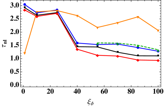
Figure 1: Nonlinearity time scales $\tau_{\rm nl}$ in $e$-folds after the end of inflation as a function of the nonminimal coupling $\xi_{\phi}$ for the benchmark Case A: $\tau_{{\rm bg},0.9}$ (blue), $\tau_{\chi_{\rm rms},0.5}$ (black), $\tau_{\phi_{\rm rms},5}$ (red), $\tau_{\rho,0.95}$ (dashed green), and $\tau_{{\rm eos},1/30}$ (orange).

To quantify the efficiency of preheating, we introduce several time-scales that characterize distinct nonlinear processes after the end of inflation:

1. $\tau_{\rm bg}$: The time at which the backreaction of the produced fluctuations starts to affect the evolution of the background field.

2. $\tau_{\chi_{\rm rms}}$: The time at which the root-mean-square (RMS) value of the $\chi$ fluctuations becomes comparable to the background inflaton value.

3. $\tau_{\phi_{\rm rms}}$: The time at which fluctuations in the $\phi$ field start growing as a result of nonlinear interactions with the produced $\chi$ fluctuations.

4. $\tau_{\rho}$: The time at which the fluctuations account for a significant fraction of the total energy density.

5. $\tau_{\rm eos}$: The time at which the universe starts expanding in an (approximately) radiation-dominated manner.

In this section we examine each of these time-scales for the “benchmark” case (Case A), with ratios of parameters given in Table 1. The results are summarized in Fig. 1, in which we can distinguish three relevant parameter regimes: $\xi_{\phi}\sim 1,10,100$. These regimes display different physical behavior because of different trade-offs between dominant contributions to $m_{{\rm eff},I}$, consistent with the analysis of the linearized perturbations in Ref. DeCross et al. (2018b). We discuss the full nonlinear dynamics of the different regimes below. In all plots the field values are shown in units of the reduced Planck mass, $M_{\text{pl}}$.

III.1.1 $\tau_{\rm bg}$: backreaction on the background field

Several recent studies of preheating in nonminimally coupled models DeCross et al. (2018a, b, c); Ema et al. (2017) and its applications to Higgs preheating Sfakianakis and van de Vis (2019); Ema et al. (2017) were based on linearized analyses, working to first order in the field fluctuations $\delta\phi^{I}$. In those studies, complete preheating was taken to be the time when the energy density of the (linearized) fluctuations became equal to the energy density of the background field. However, once a significant number of particles has been produced, the backreaction on the background field can no longer be neglected; that is, the decay of the lattice-averaged field $\langle\phi\rangle$ cannot be described by gravitational redshift alone. We define the timescale $\tau_{{\rm bg},x}$ as the moment when $\langle\phi\rangle$ (as computed on the lattice) becomes smaller than $x\cdot\varphi(t)$, where $\varphi$ is computed in the linearized analysis (which neglects backreaction, so that $\varphi(t)$ only decreases due to redshift). Here $x$ is a dimensionless parameter that encodes the amount of divergence between the (nonlinear) lattice and the (linearized) background evolution. This time-scale is indicated by the vertical blue line in Fig. 2 for $\xi_{\phi}=1$ and $\xi_{\phi}=100$, for $x=0.9$.

III.1.2 $\tau_{\chi_{\rm rms}}$: $\chi_{\rm rms}$ becomes comparable to $\langle\phi\rangle$

During preheating, parametric resonance drives the production of quanta with specific wavenumbers. Despite the inherent complexity of the underlying resonance structure, the number density of produced $\phi^{I}$-quanta can be quantified by the root-mean-square (RMS) value of the $\phi^{I}$-field on the lattice: $\phi^{I}_{\rm rms}\equiv\sqrt{\langle(\phi^{I})^{2}\rangle-\langle\phi^{I}\rangle^{2}}$. In the models considered here, the production of $\chi$-quanta is typically much more efficient than the production of $\phi$-quanta, because of the Riemann spike. We define the time-scale $\tau_{\chi_{\rm rms},x}$ as the moment when the RMS value of the $\chi$-field becomes larger than $x\cdot\langle\phi\rangle$. In Fig. 2, the vertical black line indicates $\tau_{\chi_{\rm rms},0.5}$ for $\xi_{\phi}=1$ and $\xi_{\phi}=100$.

III.1.3 $\tau_{\phi_{\rm rms}}$: $\phi_{\rm rms}$ grows as a result of rescattering

As the self-resonance in the $\phi$-field is typically much weaker than the resonance in the $\chi$ field (which is driven by the field-space curvature), rescattering of $\chi$-modes is the dominant mechanism for amplifying $\phi$-modes. This mechanism is not present in the linearized analysis, so we can quantify the strength of this effect by comparing $\phi_{\rm rms}$ as computed using the lattice results and using the linearized analysis (which neglects backreaction). The quantity $\tau_{\phi_{\rm rms},x}$ is defined as the moment when $\phi_{\rm rms}$ as computed on the lattice exceeds $x\cdot\phi_{\rm rms}$ in the linearized analysis. This time-scale does not depend solely on the efficiency of production, but also on the coupling between $\phi$- and $\chi$-modes. The time $\tau_{\phi_{\rm rms},5}$ is indicated by the vertical red line in Fig. 2.

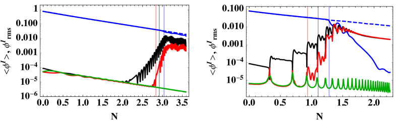
Figure 2: The behavior of various quantities in $e$-folds $N$ after the end of inflation, for Case A: the lattice-averaged background field $\langle\phi\rangle$ (blue); the background field in the linearized analysis $\varphi$ (dashed blue); $\chi_{\rm rms}$ from the lattice (black); $\phi_{\rm rms}$ from the lattice (red); and $\phi_{\rm rms}$ from the linearized analysis (green). All fields are plotted in units of the reduced Planck mass. The values of the nonminimal couplings are $\xi_{\phi}=1$ (left) and $\xi_{\phi}=100$ (right). The vertical blue, black, and red lines indicate $\tau_{{\rm bg},0.9}$, $\tau_{\chi_{\rm rms},0.5}$ and $\tau_{\phi_{\rm rms},5}$, respectively.

III.1.4 $\tau_{\rho}$: significant energy transfer

The fraction of energy density in the produced particles is an important measure of the efficiency of preheating. The time-scale $\tau_{\rho,x}$ is defined as the moment when $[1-(\rho_{\rm bg}/\rho_{\rm tot})]>x$. The plot of $\tau_{\rho,0.95}$ in Fig. 1 demonstrates that only for $\xi_{\phi}\geq 55$ are the preheating processes efficient enough to transfer as much as $95\%$ of the energy density from the background into a bath of produced particles. Fig. 3 shows $[1-(\rho_{\rm bg}/\rho_{\rm tot})]$ as a function of time for $\xi_{\phi}=1,10,25,40,55,70,85,100$ (red, magenta, black, orange, purple, dashed green, brown, blue, respectively). The time $\tau_{\rho,0.95}$ is indicated for $\xi_{\phi}=55,70,85,100$.

In the case of preheating with a simple massive inflaton field, if some energy density remains in the inflaton condensate after the phase of parametric resonance, the inflaton will eventually become the dominant constituent again, because of the faster rate at which energy density redshifts in fluctuations ($\sim a^{-4}(t)$) compared to that of the inflaton condensate ($\sim a^{-3}(t)$). We see a similar result for $\xi_{\phi}=55,70$. There the fluctuations grow by draining over $90\%$ of the energy density of the inflaton, without completely preheating the universe. After $N\simeq 1.5$ $e$-folds we see that the fractional energy in fluctuations falls. Whereas the quartic potential of the inflaton field close to the origin in the family of models we consider here might suggest that the condensate and fluctuation would redshift at the same rate ($\sim a^{-4}(t)$), two effects lead to a growth of $\rho_{\rm bg}/\rho_{\rm tot}$ and a departure from complete preheating. For nonminimal couplings $\xi>{\cal O}(10)$, the background evolves with an equation of state close to $w=0$ DeCross et al. (2018a). Furthermore, the right panel of Fig. 3 shows that during the initial growth of fluctuations, they acquire a stiff equation of state $w>1/3$ for $1.5\lesssim N\lesssim 2.5$ for $\xi_{\phi}=55,70$. Hence, even if the energy density of the condensate redshifts as $a^{-4}(t)$, the fluctuations temporarily redshift even faster.

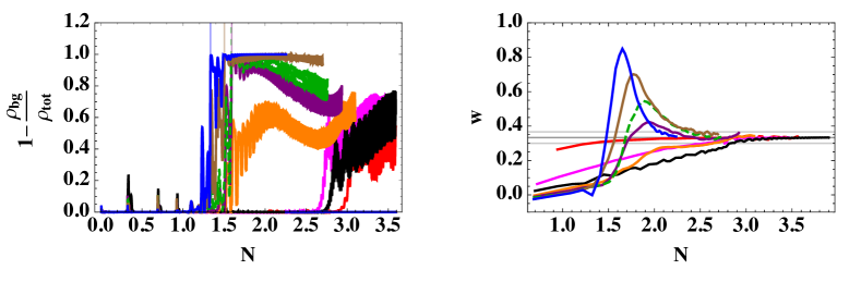
Figure 3: Left: The fraction of the energy density in produced particles $[1-(\rho_{\rm bg}/\rho_{\rm tot})]$ for Case A versus $e$-folds $N$ after the end of inflation, for $\xi_{\phi}=1,10,25,40,55,70,85,100$ (red, magenta, black, orange, purple, dashed green, brown, blue, respectively). The vertical lines indicate $\tau_{\rho,0.95}$ for $\xi_{\phi}=55,70,85,100$, in the color corresponding to the appropriate curve. Right: Equation of state for Case A, averaged over one inflaton period, for $\xi_{\phi}=1,10,25,40,55,70,85,100$ (same color coding as in the left plot).

III.1.5 $\tau_{\rm eos}$: emergence of radiation-dominated equation of state

One of the most significant potential impacts of the reheating era on observables is the evolution of the scale factor as the universe transitions from inflation (with an equation of state $w\simeq-1$) to radiation-dominated expansion (with $w=1/3$). Variations in the expansion history after inflation, encoded through time-varying $w$, affect the matching between CMB-relevant modes and the time when they first exited the Hubble radius during inflation Martin and Ringeval (2010); Mielczarek (2011); Martin et al. (2015); Munoz and Kamionkowski (2015); Creminelli et al. (2014a, b); Dai et al. (2014); Cai et al. (2015); Cook et al. (2015); Eshaghi et al. (2016); Ueno and Yamamoto (2016); Figueroa and Tanin (2019). In the case of a minimally coupled, massless inflaton field, like one governed by a quartic potential $V(\phi)\propto\phi^{4}$, the oscillations of the inflaton condensate correspond to $w=1/3$ immediately after the end of inflation, even before the production of significant numbers of higher-momentum particles. Whereas for small values of the nonminimal coupling $\xi_{\phi}$, the background evolution after inflation is similar to the minimally coupled case DeCross et al. (2018b), the behavior is significantly different for $\xi_{\phi}\gg 1$, for which the usual virial-theorem calculation for a scalar field must be modified to include a contribution from the field-space metric Kaiser and Sfakianakis (2014). As $\xi_{\phi}$ is increased, the oscillating inflaton condensate spends an increasingly long time exhibiting a matter-like equation of state, as described in detail in Ref. DeCross et al. (2018a). In that same regime of parameter space ($\xi_{\phi}\gg 1$), however, higher-momentum modes of the $\chi$-field can be efficiently produced, which will transfer energy from the inflaton condensate into a bath of radiative degrees of freedom, eventually yielding a radiation-dominated equation of state. We define the time-scale $\tau_{\rm eos}$ as the time after which the equation of state of the $\{\phi,\chi\}$ system remains close to $w=1/3$. More precisely, we define $\tau_{{\rm eos},x}$ as the time after which $|w-1/3|\leq x$, until the end of our simulations, regardless of whether $w$ is mostly controlled by the background field $\varphi$ or by the produced $\phi$ and $\chi$ particles.

III.2 Dynamics and Competition of Mass Scales

We found in the previous subsection that the universe transitions to a radiation-dominated expansion ($w\simeq 1/3$) within fewer than 3 $e$-folds, for $\xi_{\phi}$ in the range $[1,100]$. However, complete preheating — as indicated by the transfer of energy from the inflaton condensate into radiative degrees of freedom — only occurs for large nonminimal couplings, close to $\xi_{\phi}\sim 100$. Based on this behavior, combined with the linearized analysis of Ref. DeCross et al. (2018b), we can distinguish three regimes, based on the value of the nonminimal coupling $\xi_{\phi}$.

III.2.1 Small-coupling regime

We start with a value of the nonminimal coupling $\xi_{\phi}\sim 1$, in the small-coupling regime DeCross et al. (2018a). Fig. 2 shows the evolution of the spatially averaged value of the inflaton $\langle\phi\rangle$, as well as the RMS values of both fields. Initially only $\chi_{\rm rms}$ grows; $\phi_{\text{rms}}$ starts to grow in tandem with $\chi_{\text{rms}}$ as soon as the latter grows beyond $\chi_{\text{rms}}\approx 10^{-3}M_{\text{pl}}$. We see that $\langle\phi\rangle$ remains larger than the RMS values of each field, and that the expression for $\varphi$ from the linearized treatment remains an excellent approximation until 3 $e$-folds after the end of inflation. Furthermore, the averaged value of the $\chi$-field, $\langle\chi\rangle$, remains much smaller than $\langle\phi\rangle$ for the entire duration of the oscillation, confirming that the single-field attractor persists during reheating. (We consider the evolution of the covariant turn-rate below.)

The left panel of Fig. 3 shows the fraction of the total energy density in radiation modes for a range of values of $\xi_{\phi}$. Until $N=2.7$ $e$-folds after the end of inflation, the energy density is almost entirely in the background field for $\xi_{\phi}=1$. Towards the end of the simulation, at $N=3.5$ $e$-folds after the end of inflation, significant energy density has been transferred to the fluctuations, but the energy density in the inflaton condensate remains sizeable, indicating that preheating does not complete for $\xi=1$. Since the energy density in both the fluctuations and in the background redshifts approximately as $a^{-4}(t)$ for $\xi_{\phi}\sim 1$, additional couplings are needed to completely reheat the universe (perturbatively) in this case, for example a mass term for the inflaton field $\phi$ and a cubic coupling $\phi\chi^{2}$, to allow for pair-production processes $\phi\to\chi+\chi$.

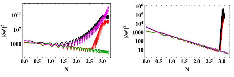
Figure 4: Growth of $|\delta\phi_{k}|^{2}$ and $|\delta\chi_{k}|^{2}$ for Case A in units of $M_{\rm pl}$ for $k\approx 3H_{\rm end}$ (left) and $k\approx 11H_{\rm end}$ (right), with $\xi_{\phi}=1$. The red (black) line shows the evolution of $|\delta\phi_{k}|^{2}$ ($|\delta\chi_{k}|^{2}$) on the lattice, and the green (magenta) dashed lines show the corresponding results in the linearized analysis.

We can account for the behavior shown in Fig. 3 by investigating the growth of $\phi_{\text{rms}}$ and $\chi_{\text{rms}}$ in more detail. Fig. 4 shows the evolution of the modes $k\approx 3\,H_{\rm end},11\,H_{\rm end}$ as computed on the lattice and in a linearized treatment. (We discuss how to make such wavenumber-specific comparisons of lattice and linearized treatments in Appendix C.) In the left panel, we see a weak parametric resonance of the $\chi$ fluctuations for small wavenumbers around $k=3H_{\rm end}$. This can be explained from the behavior found in Ref. DeCross et al. (2018b), in which the Fourier decomposition of the background field $\varphi(t)$ and the Floquet structure of the resonances were discussed (to linear order in fluctuations). It was found that the Fourier modes of $\varphi(t)$ collapse to a pure sinusoidal oscillation for $\xi_{\phi}\simeq 1$. For that same regime of $\xi_{I}$, the instability bands of the $\chi$ fluctuations are significantly reduced in width (“pinched”), thereby leading to a set of very narrow instability bands. This is exactly mirrored by the behavior in the left panel of Fig. 4, in which the growth in $|\delta\chi_{k}|^{2}$ is caused by a narrow resonance at $k\approx 3H_{\text{end}}$. At $2.5$ $e$-folds, $|\delta\phi_{k}|^{2}$ starts to grow as a result of rescattering of $\delta\chi_{k}$-modes into $\delta\phi_{k}$-modes, an effect that is not captured by the linearized analysis. The right panel of Fig. 4 shows that modes with $k\approx 11H_{\text{end}}$ start to grow somewhat later, at 2.8 $e$-folds, solely as a result of rescattering. From Fig. 2 we see that backreaction of the produced particles on $\langle\phi\rangle$ causes a deviation from the linearized treatment by $\tau_{\rm bg}\simeq 3$ $e$-folds after the end of inflation for $\xi_{\phi}\simeq 1$, which is consistent with the moment at which the resonance in $\delta\chi_{k}$ shuts off in the left panel of Fig. 4.

III.2.2 Intermediate-coupling regime

Interesting effects arising from the competition between the dominant terms in the effective mass of $\chi$ fluctuations are found in the case of $\xi_{\phi}\sim 10$, which falls in the intermediate-coupling regime DeCross et al. (2018a). In this regime, the two main contributions to the effective mass-squared of the $\chi$ fluctuations, the contribution $m_{\chi,1}^{2}$ from the potential and the contribution $m_{\chi,2}^{2}$ from the field-space (Riemann) curvature, are similar in size at the onset of reheating. Since $m_{1,\chi}^{2}$ and $m_{2,\chi}^{2}$ oscillate out of phase, preheating is initially suppressed. This effect was identified in Ref. DeCross et al. (2018c) (in a linearized analysis) and appears in Fig. 5 as the initial behavior of $\chi_{\rm rms}$ for $N\lesssim 2$ $e$-folds after the end of inflation: no resonant growth occurs. Since $m_{\chi,1}^{2}$ grows faster than $H^{2}$, whereas $m_{\chi,2}^{2}\propto H^{2}$ DeCross et al. (2018c), $m_{1,\chi}^{2}$ comes to dominate after the so-called cross-over time, which was computed in Ref. DeCross et al. (2018c). The relation $m_{\chi,1}^{2}\gg m_{\chi,2}^{2}$ leads to a period of normal parametric resonance, which is shown in Fig. 5. The case $\xi_{\phi}=1$ exhibited a resonance for small $k$, but for $\xi_{\phi}=10$ the resonant growth of $\chi_{k}$ occurs for values of the comoving wavenumber up to $k\lesssim 20\,H_{\text{end}}$.

We can see in Fig. 5 that $\phi_{\text{rms}}$ starts to grow (and diverge from the linearized analysis) around $2.5$ $e$-folds, when $\langle\chi\rangle={\cal O}(10^{-3})M_{\rm pl}$, similar to the case of $\xi_{\phi}=1$. At the end of the simulation the RMS values of the two fields are comparable. The energy density in the inflaton condensate $\langle\phi\rangle$ at the end of our simulation (approximately $3$ $e$-folds after the end of inflation) still comprises around $30\%$ of the total energy density of the universe, hence preheating in this case does not complete.

The case $\xi_{\phi}=25$ deserves special attention, since it displays two kinds of resonant behavior. Initially, the Riemann contribution to the effective mass, $m_{\chi,2}^{2}$, is dominant. This leads to amplification of $\chi$ fluctuations every time that the background field crosses the origin ($\varphi=0$), where the field-space curvature exhibits a large local increase (the “Riemann spike”). This resonant behavior was previously identified in the large-coupling regime and studied extensively (in a linearized analysis) in Refs. DeCross et al. (2018a, b, c).

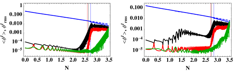
Figure 5: The lattice-averaged background field $\langle\phi\rangle$ (blue), the background field in the linearized analysis $\varphi$ (dashed blue), $\chi_{\rm rms}$ from the lattice (black), $\phi_{\rm rms}$ from the lattice (red) and $\phi_{\rm rms}$ from the linearized analysis (green) for Case A, versus $e$-folds $N$ after the end of inflation. The values of the nonminimal couplings are $\xi_{\phi}=10$ (left) and $\xi_{\phi}=25$ (right). The vertical blue, black, and red lines indicate $\tau_{{\rm bg},0.9}$, $\tau_{\chi_{\rm rms},0.5}$ and $\tau_{\phi_{\rm rms},5}$, respectively.

Fig. 5 indeed shows an increase of $\chi_{\text{rms}}$ for $N\lesssim 1.5$ $e$-folds after the end of inflation. At 1.5 e-folds after the end of inflation, the growth in $\chi_{\text{rms}}$ shuts off. This is a result of the decrease of $m_{\chi,2}^{2}$ compared to $m_{\chi,1}^{2}$, causing destructive interference, as described above for the $\xi_{\phi}=10$ case. Up to this time, no significant amount of energy has been transferred to the $\chi$ fluctuations yet. Backreaction is not yet effective, so the linearized approximations for $\chi_{\text{rms}}$ and $\langle\phi\rangle$ remain valid. At 2.5 $e$-folds after the end of inflation, $m_{\chi,2}^{2}$ has redshifted enough to render destructive interference between the potential and Riemann terms ineffective, and a period of ordinary parametric resonance starts. This again leads to growth of $\chi_{\text{rms}}$, which quickly drives growth of $\phi_{\text{rms}}$ from rescattering.

III.2.3 Large-coupling regime

The value $\xi_{\phi}=100$ places the system in the large-coupling regime DeCross et al. (2018a), which is characterized by a large amplification of $\chi$ fluctuations. Preheating concludes after a few oscillations (5-6 zero-crossings) of the background field, as shown in Figs. 2 and 3, and backreaction becomes significant even more quickly.

As validated by the results plotted in Fig. 2, the background inflaton field $\langle\phi\rangle$ starts to be affected by backreaction effects after the first two oscillations, and becomes completely subdominant shortly thereafter. The variances of the two fields $\phi$ and $\chi$ are almost identical at late times, signaling a kind of “equipartition” phenomenon, which can be attributed to the tendency of the system to thermalize. The energy density remaining in the background field is several orders of magnitude smaller than the total energy density of the system, hence we can safely conclude — within the limitations of the resolution of our lattice — that the Universe completely preheats into an equilibrated ensemble of $\chi$ and $\phi$ particles for $\xi_{\phi}=100$. Furthermore, the lattice-averaged value of the $\chi$ field, $\langle\chi\rangle$, which plays the role of the background $\chi$ field in a linearized analysis, remains subdominant to $\langle\phi\rangle$ until the end of the simulation, at which point both are vastly subdominant to the corresponding variances: $\langle\chi\rangle<\langle\phi\rangle\ll\phi_{\rm rms}\simeq\chi_{\rm rms}$.

III.2.4 Preheating, Rescattering & Observables

The usual comparison of predictions for primordial observables from inflationary models and high-precision observations hinges on the freeze-out of the adiabatic fluctuations after they exit the Hubble radius during inflation. However, this can be violated in multifield models of inflation, due to interactions with isocurvature modes. The interplay between isocurvature and adiabatic modes has been studied extensively in the literature, mostly focusing on the inflationary regime. (For reviews, see Refs. Wands (2008); Gong (2016).) In the class of multifield models we study here, the generic single-field attractor behavior strongly suppresses the amplification of isocurvature modes during inflation and the generation of significant non-Gaussianities; these multifield effects occur only for highly fine-tuned choices of couplings and initial conditions Kaiser et al. (2013); Kaiser and Sfakianakis (2014); Schutz et al. (2014).

The adiabatic and entropic (isocurvature) modes are described by the gauge-invariant curvature perturbation $\mathcal{R}_{c}$ and the normalized entropy perturbation $\mathcal{S}$. On super-horizon scales, the evolution of these petrurbations can be approximated as

$${d{\mathcal{R}_{c}}\over dN}\simeq{2\omega\over H}{\mathcal{S}}\,,\quad{d{\mathcal{S}}\over dN}\simeq{\beta}{\mathcal{S}}\,,$$ (40)

where $\omega$ is the (covariant) turn-rate of the background trajectory and $\beta$ depends on the slow-roll parameter $\epsilon$, the effective masses of the adiabatic and isocurvature fluctuations, and the turn-rate $\omega$ Kaiser et al. (2013). In the case of preheating, super-horizon isocurvature modes (with $k\to 0$) can be excited, due to the super-horizon correlation length of the inflaton condensate Bassett et al. (1999a, b, 2000); Gordon et al. (2000). If the background trajectory is turning, power from the isocurvature modes can be imprinted on the adiabatic modes, following Eq. (40). Since we observe significant growth of isocurvature fluctuations after the end of inflation, across a large range of scales $k$, it is imperative to thoroughly check whether predictions for CMB observables are protected or spoiled by interactions during the preheating phase.

In order to assess the background motion during preheating and identify possible deviations from the single-field attractor, we compute the covariant turn-rate for the system in field-space and consider the ratio $|\omega|/H$ as we vary $\xi_{\phi}$. If $|\omega|/H\ll 1$, the transfer of energy from the isocurvature to the adiabatic modes remains suppressed and thus, at least in the regime of validity of Eq. (40), the adiabatic modes on scales relevant to CMB observations do indeed remain frozen during preheating.

In the typical covariant approach for multifield models (which we followed in Refs. Kaiser et al. (2013); Greenwood et al. (2013); Kaiser and Sfakianakis (2014); Schutz et al. (2014)), when working to linear order in fluctuations, one defines the length of the background-field velocity vector

$$|\dot{\varphi}^{I}|\equiv\dot{\sigma}=\sqrt{{\cal G}_{IJ}\,\dot{\varphi}^{I}\,\dot{\varphi}^{J}}\,,$$ (41)

in terms of which one may define the unit vector

$$\hat{\sigma}^{I}\equiv\frac{\dot{\varphi}^{I}}{\dot{\sigma}}.$$ (42)

The covariant turn-rate vector is then given by

$$\omega^{I}\equiv{\cal D}_{t}\hat{\sigma}^{I}=-\frac{1}{\dot{\sigma}}V_{,K}\,\hat{s}^{IK}\,,$$ (43)

where the last expression follows upon using the equation of motion for the homogeneous background fields $\varphi^{I}$, and the quantity $\hat{s}^{IK}\equiv{\cal G}^{IK}-\hat{\sigma}^{I}\hat{\sigma}^{K}$ projects into directions of field-space orthogonal to $\hat{\sigma}^{I}$. Using the properties of the projectors $\hat{s}^{IK}$ Kaiser et al. (2013), it is straightforward to show that

$$|\omega^{I}|=\frac{1}{\dot{\sigma}^{2}}\left[V_{,K}\,V_{,L}\left(\dot{\sigma}^{2}{\cal G}^{KL}-\dot{\varphi}^{K}\,\dot{\varphi}^{L}\right)\right]^{1/2}\,.$$ (44)

The only term in Eq. (44) that becomes problematic during preheating is the coefficient $1/\dot{\sigma}^{2}$, outside the square brackets, since during preheating $\dot{\sigma}$ repeatedly oscillates to zero. However, if we perform a time-average of this coefficient over each oscillation of the inflaton condensate, then the expression for $|\omega|=|\omega^{I}|$ in Eq. (44) remains well-behaved. To apply Eq. (44) to our lattice simulations, we evaluate all terms that depend on the spatially homogeneous quantities $(\varphi^{I},\dot{\varphi}^{I})$ by substituting the corresponding spatial averages on the lattice.

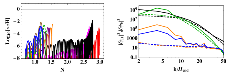
Figure 6: Left: The covariant turn-rate $|\omega|$ normalized by the Hubble scale $H$ for Case A and different values of the nonminimal coupling in the range $1\leq\xi_{\phi}\leq 100$. Color coding as in Fig. 3. We see that in all cases $|\omega|<0.1H$. Note that, as explained in the main text, we only consider the turn-rate for times such that $\langle\phi^{I}\rangle>\phi^{I}_{\rm rms}$ for at least one component $I$, since this defines the regime of validity of Eqs. (40) and (44). Right: The power spectrum for $\phi$ (dashed) and $\chi$ (solid) fluctuations for $\xi_{\phi}=10$ and $N=2.3,2.4,2.7,3.0$ (blue, orange, green, black, respectively). We see that when backreaction becomes significant the two spectra become nearly indistinguishable.

Eqs. (40) and (44) only apply when one may identify a well-defined background solution. In the context of our lattice simulations, Eqs. (40) and (44) remain well-defined for times such that the lattice-averaged value for at least one component of $\phi^{I}=\{\phi,\chi\}$ remains greater than the corresponding RMS value for that component: $\langle\phi^{I}\rangle>\phi_{\rm rms}^{I}$ for at least one component $I$. (We consider this condition further in Section III.3 when we examine Case D, with positive ellipticity.) Subject to this criterion, we find the results for $\omega$ (normalized by the Hubble rate) shown in the left panel of Fig. 6. We see that for all values of $\xi_{\phi}$ under consideration, the turn-rate remains much smaller than the Hubble scale throughout the preheating phase, even as $H$ itself falls over time.

A second criterion for whether preheating dynamics could affect predictions for primordial observables concerns how quickly the system reaches the adiabatic limit Elliston et al. (2011); Meyers and Tarrant (2014); Elliston et al. (2014); Renaux-Petel and Turzynski (2015). The right panel of Fig. 6 shows that soon after the $\chi$ particles are produced, they rescatter efficiently, producing nearly identical spectra for the $\delta\chi_{k}$ and $\delta\phi_{k}$ modes. (This is consistent with our finding in Fig. 5 that $\phi_{\rm rms}\simeq\chi_{\rm rms}$ within a few $e$-folds after the end of inflation for $\xi_{I}\sim{\cal O}(10)$.) Although an accurate simulation of thermalization is beyond the scope of this work, Fig. 6 indicates that an “equipartition” of energy density quickly emerges between the two fields, which can be considered a precursor to thermalization Micha and Tkachev (2003, 2004); McDonough (2020). Within the first few $e$-folds after the end of inflation, the fluctuations in both the $\chi$ and $\phi$ fields lose all information about the wavenumber-dependent structure of the initial resonances, and begin to approach quasi-thermal spectra. Since the turn-rate remains tiny up through the time that quasi-thermal spectra emerge, we conclude that the predictions for observables such as the spectral index $n_{s}$ and the tensor-to-scalar ratio $r$ from models of the type in Case A, across a wide range of nonminimal couplings $\xi_{\phi}$, remain unaffected by the rapid growth of isocurvature fluctuations after the end of inflation.

In sum, we have shown that for the “generic” benchmark case (Case A), preheating becomes more efficient as we increase $\xi_{\phi}$. Different dynamics occur for different regimes of $\xi_{\phi}$, governed by the interplay between contributions to $m_{{\rm eff},I}^{2}(t)$ from the potential and the field-space structure. Several nonlinear processes unfold over distinct time-scales, some of which are strongly correlated with each other. For large values of the nonminimal coupling, $\xi_{\phi}\sim 100$, we find that each of these processes is essentially completed within $N_{\rm reh}\lesssim 2.5$ $e$-folds after the end of inflation.

III.3 Parameter Dependence

Having presented a detailed analysis of the preheating dynamics for the “benchmark” case (Case A in Table 1), we now examine how preheating depends on the potential topography. Ref. DeCross et al. (2018b) analyzed parametric resonance for this family of models to linear order in fluctuations, and identified distinct characteristic behavior across parameter space. Building on the intuition afforded by that analysis, we now examine the fully nonlinear dynamics of each of the four characteristic cases (B-D) shown in Table 1, and compare them with the benchmark Case A.

Fig. 7 shows the dependence of the time-scales $\tau_{\rho}$ and $\tau_{\text{bg}}$ on the value of the nonminimal coupling $\xi_{\phi}$ for each of the five characteristic cases (A-E). We see that complete energy transfer is only possible for $\xi_{\phi}\gtrsim 55$, except for Case D (positive ellipticity), which is particularly efficient. Preheating in Case C (negative ellipticity), on the other hand, proceeds slowly, and complete energy transfer does not occur even for large $\xi_{\phi}$. The backreaction of produced particles on the evolution of the inflaton condensate is also significantly slower for Case C compared to the other cases. Despite differences among the cases, however, we again find the general trend that preheating becomes more efficient as the values of the nonminimal couplings $\xi_{I}$ increase, and that (apart from Case C with negative ellipcticity) the relevant, nonlinear preheating processes are completed within $N_{\rm reh}\lesssim 2$ in the limit $\xi_{\phi}\sim 100$.

Fig. 8 shows the evolution of the equation of state, averaged over each oscillation of the $\phi$ field. The approach of the equation of state to radiation-dominated expansion ($w=1/3$) proceeds similarly to the benchmark Case A across these cases (compare with Fig. 3, right panel), except for Case C (negative ellipticity). We explore each of these cases in more detail below.

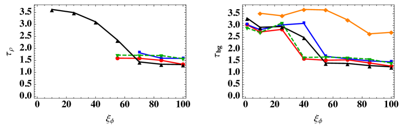
Figure 7: $\tau_{\rho,0.95}$ (left) and $\tau_{\text{bg},0.9}$ (right), for all five cases. Color coding is Case A (benchmark case, red), Case B (symmetric couplings, blue), Case C (negative ellipticity, orange), Case D (positive ellipticity, black) and Case E (zero ellipticity, dashed green).

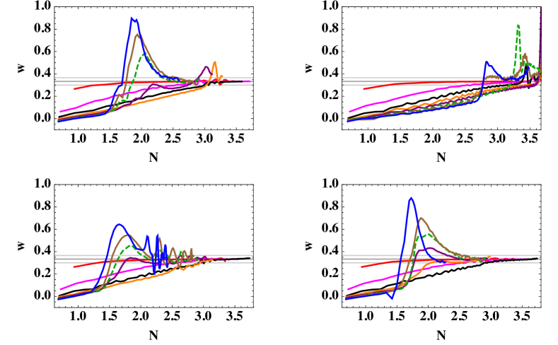
Figure 8: Equation of state for Case B (symmetric couplings, top left), Case C (negative ellipticity, top right), Case D (positive ellipticity, bottom left) and Case E (zero ellipticity, bottom right). Color coding as in Fig. 3. The averaging window is always the period of the $\phi$-field. For Case D, the lattice-averaged value of the $\chi$-field becomes larger than the $\phi$-field for some values of $\xi_{\phi}$. The rapid oscillations of $w$ for $\xi_{\phi}=85,100$ can be removed by switching to an integration window corresponding to the oscillations of $\langle\chi\rangle$ once $\langle\chi\rangle$ dominates over $\langle\phi\rangle$.

III.3.1 Case B: Symmetric Couplings

A physically important case is that of symmetric couplings ($\xi_{\phi}=\xi_{\chi}$ and $\lambda_{\phi}=g=\lambda_{\chi}$), which arises if the model obeys an $SO(2)$ (or higher) symmetry. This would be a proxy for Higgs inflation, if one focused on the scalar degrees of freedom and neglected the effects of the gauge bosons DeCross et al. (2018c). (See Ref. Sfakianakis and van de Vis (2019) for a detailed computation of preheating in Higgs inflation; compare with Refs. Bezrukov et al. (2009); Garcia-Bellido et al. (2009); Dufaux et al. (2010); Repond and Rubio (2016).) As shown in Ref. Nguyen et al. (2019), the symmetric case (Case B) has a similar preheating behavior to the benchmark case (Case A) for $\xi_{\phi}=1,10,100$, although preheating occurs with a minor delay in the symmetric case, with a slightly longer time-scale before significant mode amplification dominates the dynamics.

Figure 8 shows the averaged equation of state for the symmetric Case B. We see a similar trend to the benchmark Case A: a temporarily stiff equation of state for large values of $\xi_{\phi}$, which quickly asymptotes to a radiation-dominated one with $w\simeq 1/3$. However, for $\xi_{\phi}=40$, there emerges a late increase in $w$ after $N=3$ $e$-folds, whereas for $\xi_{\phi}=55$ the equation of state exhibits a temporary local maximum at $N\simeq 2$ and then exceeds $w=1/3$ at $N\simeq 3$. This behavior can be easily understood by considering the field variances for these values of $\xi_{\phi}$, as shown in Fig. 9.

For both $\xi_{\phi}=40,55$ we see an early period of amplification of the $\chi$ field driven by the field-space curvature (Riemann) term $m_{2,\chi}$ in the effective mass. This resonance is too weak to completely preheat the universe and eventually shuts off. At later times, after the Riemann contribution has redshifted to become a subdominant contribution to $m_{\rm eff,\chi}$, a period of ordinary (potential-driven) parametric resonance drives a significant transfer of energy from the inflaton into higher-momentum $\chi$ modes. This causes the late-time peak in the equation of state. In the case $\xi_{\phi}=55$ the initial resonance at $N\simeq 1.5$ is strong enough to drain sufficient energy from the inflaton condensate and drive a local peak in the equation of state. It is interesting to note that the late-time parametric resonance occurs in the $\phi$ field. This two-stage parametric resonance process is similar to that found above for the benchmark Case A for $\xi_{\phi}\sim 25$ (see Section III.2.2).

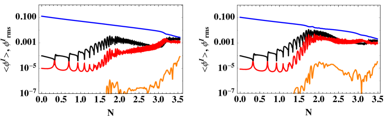
Figure 9: The lattice-averaged fields and corresponding RMS values versus $e$-folds after the end of inflation for Case B (symmetric couplings), with $\xi_{\phi}=40,55$ (left and right, respectively). We have used interpolation between the peaks of $\langle\phi\rangle$ (blue), $\langle\chi\rangle$ (orange) and $\phi_{\text{rms}}$ (red), $\chi_{\text{rms}}$ (black).

III.3.2 Case C: Negative Ellipticity

The negative ellipticity case (with $\varepsilon=(\xi_{\phi}-\xi_{\chi})/\xi_{\phi}<0$) shows the largest deviation from the benchmark Case A, as well as the other cases that we explore here. This can be seen in the time-scales shown in Fig. 7 as well as the equation of state shown in Fig. 8. These results are consistent with our previous findings from our linearized analysis DeCross et al. (2018b), in which we had found that a large negative ellipticity suppresses the Floquet structure of the model, almost eliminating all resonance bands. This is verified by the fully nonlinear lattice simulations, in which we find that complete preheating is not reached, even for $\xi_{\phi}=100$, contrary to all other cases. Furthermore, the averaged equation of state remains $w<1/3$ through $N\approx 2.5$ $e$-folds after the end of inflation. In this case, we find a modest, late-time parametric resonance, after the Rieman spike has redshifted enough to be insignificant.

It is interesting to note that for small values of $\xi_{\phi}\lesssim 25$, the late-time resonance occurs in the $\phi$ field, while for larger values of $\xi_{\phi}$ the late-time resonance is driven primarily by the $\chi$ field; in the latter case, the resonance is driven predominantly by the potential contribution to the effective mass, $m_{1,\chi}$, rather than from the field-space curvature contribution, $m_{2,\chi}$. Fig. 10 shows the behavior of the spatially averaged fields and their corresponding RMS values for two characteristic values of $\xi_{\phi}$ to illustrate these two different regimes.

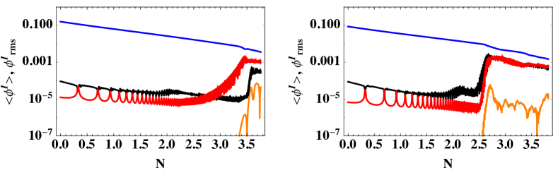
Figure 10: The lattice-averaged fields and corresponding RMS values versus $e$-folds after the end of inflation for Case C (negative ellipticity), with $\xi_{\phi}=25,85$ (left and right, respectively). We have used interpolation between the peaks of $\langle\phi\rangle$ (blue), $\langle\chi\rangle$ (orange) and $\phi_{\text{rms}}$ (red), $\chi_{\text{rms}}$ (black).

III.3.3 Case D: Positive Ellipticity

We considered the case of positive ellipticity within a linearized analysis in Ref. DeCross et al. (2018b), and found that positive ellipticity led to stronger violation of the adiabaticity condition and, correspondingly, larger resonance bands than models with symmetric couplings, yielding efficient preheating. We find comparable behavior in our nonlinear lattice simulations as well. For example, Fig. 7 shows that $\tau_{\rho}$ occurs more quickly for Case D than for any of the other cases in the regime of large couplings $\xi_{\phi}\geq 55$. Even more striking, only for Case D does preheating lead to a significant transfer of energy density from the inflaton condensate into radiative degrees of freedom for smaller nonminimal couplings, $\xi_{\phi}\sim{\cal O}(10)$.

As shown in Fig. 8, the equation of state $w$ for Case D shows large, persistent oscillations around $w\simeq 1/3$ after the first $1.5$ $e$-folds. As noted above, the equation of state shown in Fig. 8 in each case was averaged over an oscillation period of the inflaton condensate, $\langle\phi\rangle$. To understand the large oscillations in $w$ for Case D, it suffices to consider the dynamics of this model with $\xi_{\phi}=85$. The left panel of Fig. 11 shows the lattice-average field values $\langle\phi\rangle$ and $\langle\chi\rangle$ as well as the corresponding variances $\phi_{\rm rms}$ and $\chi_{\rm rms}$. We see that after a significant energy transfer has occurred from the inflaton condensate into radiative modes, the lattice-averaged (background) trajectory of the system is primarily aligned along the $\chi$ axis. After this point, the dominant frequency for the system is that of $\langle\chi\rangle$ oscillations, rather than the $\langle\phi\rangle$ oscillations. If we average the equation of state $w$ within a window set by the oscillation frequency of $\langle\chi\rangle$, we find that $w$ approaches $w=1/3$ in a way more comparable to that of the benchmark Case A.

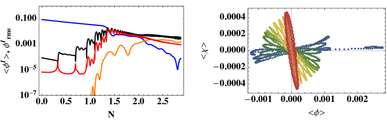
Figure 11: Left: The lattice-averaged fields and corresponding RMS values versus $e$-folds after the end of inflation for Case D (positive ellipticity) with $\xi_{\phi}=85$. We have used interpolation between the peaks of $\langle\phi\rangle$ (blue), $\langle\chi\rangle$ (orange), $\phi_{\text{rms}}$ (red), and $\chi_{\text{rms}}$ (black). Right: The lattice-averaged motion in the $\phi-\chi$ plane between 1.3 and 2.7 $e$-folds after the end of inflation. Later times correspond to redder colors.

The apparent departure from the single-field attractor along $\langle\chi\rangle\simeq 0$ raises the question of whether predictions for CMB observables in this case might be altered by post-inflationary dynamics. Even for Case D, however, the strong agreement between predictions from this family of models and CMB observations remains protected, despite the violent energy exchange after the end of inflation, for at least two reasons.

First, we note that the power spectra of the $\phi$ and $\chi$ fields have “equlibrated” (akin to the spectra shown in Fig. 6) prior to the time when $\langle\chi\rangle$ dominates over $\langle\phi\rangle$, hence no information can be transmitted coherently from subhorizon to superhorizon scales. (In Fig. 11 this effect is consistent with $\phi_{\rm rms}\simeq\chi_{\rm rms}$ by $N\simeq 1.3$ $e$-folds after inflation.) Although a detailed discussion of equilibration and thermalization is beyond the scope of the present work, it is clear from such spectra that the final distribution of power among the $\phi$ and $\chi$ fluctuations is vastly different from that following the initial parametric resonance. Strong rescattering effects appear to have largely erased any wavenumber-dependent information and yielded spectra that are similar among the $\phi$ and $\chi$ fields.

Second, we have found that in all cases, $\chi_{\rm rms}\gg\langle\chi\rangle$ by the time $\chi_{\rm rms}\simeq\phi_{\rm rms}$. This implies that the evolution of the lattice-averaged quantity $\langle\chi\rangle$ is a statistical phenomenon that assumes different values in each Hubble patch, rather than a coherent motion of the $\chi$ field across superhorizon scales. In order to examine this, we performed simulations with different seeds for the fluctuations, all taken from the same distribution. Fig. 12 shows the results for three such simulations. We see that while the variances are identical, the lattice-averaged values depend strongly on the specific seed. Hence different Hubble patches, which in our simulation can be simulated by selecting different seeds, will develop different values of $\langle\chi\rangle$. This suggests that no $\chi$ condensate exists with superhorizon correlations, which in turn implies that the power in low-$k$ modes cannot be imprinted onto the adiabatic perturbations on CMB-relevant scales after the end of inflation.

More fundamentally, while our analysis shows that predictions for CMB observables in this family of models remain unaffected by preheating, we emphasize that the formulas in Eq. (40) that describe the superhorizon evolution of adiabatic and isocurvature perturbations presuppose the existence of a well-defined, coherent background motion, in terms of which one may define the covariant turn-rate $\omega$, as in Eq. (44). When the RMS of the fields far exceed the lattice-averaged field values, the existence of a coherent background motion becomes ill-defined. How to modify simple relations like Eq. (40) for evolution deep into the nonlinear regime remains an interesting question, beyond the scope of the present work.

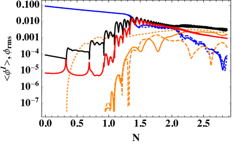
Figure 12: Lattice-averaged field values and corresponding RMS values for Case D (positive ellipticity) with $\xi=85$ for three different seeds for the initial fluctuations. Color coding is the same as in the left panel of Fig. 11. The three different seeds are shown in solid, dashed and dotted. Note that across the three seeds, the late-time values of $\phi_{\rm rms}$ (red) and $\chi_{\rm rms}$ (black) remain consistent, whereas the late-time values of $\langle\chi\rangle$ (orange) differ significantly, indicating a lack of superhorizon coherence of the $\chi$ field after the end of inflation.

III.3.4 Case E: Zero Ellipticity

We conclude our analysis with Case E (zero ellipticity), for which $\xi_{\phi}=\xi_{\chi}$, but for which, in general, $\lambda_{\phi}\neq g\neq\lambda_{\chi}$ (see Table 1). Because the couplings in the Jordan-frame potential do not equal each other, Case E is distinct from the symmetric Case B. Nonetheless, we see that the phenomenology for Case E is largely indistinguishable from the benchmark Case A, both in terms of the relevant time-scales (Fig. 7) as well as the evolution of the equation of state (Figs. 3 & 8). This result is not surprising, since any non-adiabatic behavior caused by the Riemann spike in $m_{2,\chi}$ is not very sensitive to small changes among the couplings in the Jordan-frame potential. The Riemann spike, after all, derives from the curvature of the field-space manifold, which depends only on the nonminimal couplings $\xi_{I}$.

IV Conclusions

Post-inflation reheating is a critical phase in the early history of our universe, connecting the era of primordial inflation with standard Big Bang evolution. The energy density that had driven accelerated expansion during inflation must be dispersed rapidly into a hot, thermal bath of Standard Model (and perhaps Dark Matter) particles, and the equation of state must assume a radiation-dominated form. Any significant delay between the end of inflation and the conclusion of reheating would have implications for the comparison of predictions for observables and high-precision measurements, by altering the expansion history of the early universe Bassett et al. (2006); Allahverdi et al. (2010); Frolov (2010); Amin et al. (2014); Lozanov (2019). Yet the principal physical processes during the reheating phase — energy transfer from the inflaton condensate into higher-momentum particles, emergence of a radiation-dominated equation of state, and thermalization of the produced particles at an appropriately high temperature — can unfold according to their own distinct time-scales, which depend in different ways on model parameters.

In this work we have examined the post-inflation phase in a family of models that incorporate realistic features from high-energy theory: multiple interacting scalar degrees of freedom, and nonminimal couplings between those fields and the space-time curvature. We have investigated several distinct nonlinear processes in these models using lattice simulations, and explored how the relevant time-scales vary across parameter space. Across all the variations within this family of models, we consistently find efficient preheating in the limit of large nonminimal couplings $\xi_{I}\sim{\cal O}(100)$, with each of the requisite preheating effects (energy transfer, radiation-dominated equation of state, and onset of thermalization) completed within $N_{\rm reh}\lesssim 3$ $e$-folds after the end of inflation. Moreover, across the variations in models and regions of parameter space, inflationary predictions for observable features in the cosmic microwave background radiation remain unaffected by the violent post-inflationary dynamics, thereby protecting the close match Kaiser and Sfakianakis (2014) between these models and the latest observations.

In general, the post-inflationary behavior of most models within this family behave in comparable ways to the “benchmark” or generic case on which we first focused (Case A) Nguyen et al. (2019). We found significant deviations from the benchmark case only for large, negative ellipticity (Case C), which can arise if there is a misalignment between the dominant direction in field-space along which the system evolves and the larger of the nonminimal couplings, $\xi_{I}$. In such cases, the parametric resonances that are typical of preheating become quenched. We further identified more modest differences from the benchmark case for large, positive ellipticity (Case D), in which particle production was even more efficient than average. In that case, the superhorizon coherence of the inflaton condensate was lost even more quickly than in more “generic” cases.

A physical effect that we have not considered in this work, but which could have interesting consequences for preheating in particular regions of parameter space, arises from coupled metric perturbations. In Ref. DeCross et al. (2018c) the detailed effects of the various contributions to the effective masses $m_{\rm eff,\phi}^{2}$ and $m_{\rm eff,\chi}^{2}$ were analyzed for this family of models to linear order in the perturbations. The coupled metric perturbations were shown to affect the adiabatic fluctuations ($\delta\phi$) for low wavenumbers (super-horizon modes, with $k<aH$). On the other hand, in these models the growth of isocurvature modes typically occurs efficiently across a wide range of wavenumbers, and is typically more efficient than the growth of adiabatic modes for large values of the nonminimal couplings $\xi_{I}\gg 1$. We therefore expect that the effect of coupled metric perturbations may be most pronounced in cases with $\xi_{I}\gg 1$, in those regions of parameter space in which the growth of isocurvature modes is suppressed due to a negative ellipticity, as in Case C; otherwise we expect effects from metric perturbations to remain subdominant, compared to the nonlinear field dynamics analyzed here. Recently, the limitations of linearized gravity for treating violent processes such as preheating has been discussed, for example in Ref. Giblin and Tishue (2019). A full numerical treatment of gravitational effects in preheating in this family of models remains the subject of further research.

Other natural extensions of this work would include coupling the scalar fields to higher-spin fields, including both fermions Greene and Kofman (1999, 2000); Peloso and Sorbo (2000); Tsujikawa et al. (2000); Adshead and Sfakianakis (2015); Adshead et al. (2018a); Repond and Rubio (2016) and gauge bosons Davis et al. (2001); Garcia-Bellido et al. (2004); Braden et al. (2010); Allahverdi et al. (2011); Deskins et al. (2013); Adshead et al. (2015, 2017); Cuissa and Figueroa (2019), and exploring possible observational consequences, such as the amplification of gravitational waves during preheating. (See, e.g., Refs. Adshead et al. (2018b); Lozanov and Amin (2019) and references therein.) In addition, although several quite distinct families of “attractor” models of inflation produce comparable predictions for CMB spectra if one only considers their dynamics during inflation Christodoulidis et al. (2019a, b), some of these other models (beyond the family we studied here) would likely not feature such efficient preheating Iarygina et al. (2020). Studies like this one may therefore begin to differentiate among competing families of models and clarify how predictions for CMB observables might be affected by distinct reheating scenarios.

Appendix A Field-Space Metric and Related Quantities

Given $f(\phi^{I})$ in Eq. (11) for a two-field model, the field-space metric in the Einstein frame, Eq. (5), takes the form

$${\cal G}_{IJ}=\left(\frac{M_{\rm pl}^{2}}{4f^{2}}\right)\begin{pmatrix}2f+6\xi_{\phi}^{2}\phi^{2}&6\xi_{\phi}\xi_{\chi}\phi\chi\\ 6\xi_{\phi}\xi_{\chi}\phi\chi&2f+6\xi_{\chi}^{2}\chi^{2}\end{pmatrix}\,,$$ (45)

where $\phi^{I}\equiv\{\phi,\chi\}$. The inverse metric is

$${\cal G}^{IJ}=\left(\frac{2f}{M_{\rm pl}^{2}C}\right)\begin{pmatrix}2f+6\xi_{\chi}^{2}\chi^{2}&-6\xi_{\phi}\xi_{\chi}\phi\chi\\ -6\xi_{\phi}\xi_{\chi}\phi\chi&2f+6\xi_{\phi}^{2}\phi^{2}\end{pmatrix}\,,$$ (46)

where $C(\phi^{I})$ is defined as

$$\begin{split}C(\phi,\chi)&\equiv M_{\rm pl}^{2}+\xi_{\phi}(1+6\xi_{\phi})\phi^{2}+\xi_{\chi}(1+6\xi_{\chi})\chi^{2}\\ &=2f+6\xi_{\phi}^{2}\phi^{2}+6\xi_{\chi}^{2}\chi^{2}.\end{split}$$ (47)

The Christoffel symbols for this field space take the form

$$\begin{split}\Gamma^{\phi}_{\>\>\phi\phi}&=\frac{\xi_{\phi}(1+6\xi_{\phi})\phi}{C}-\frac{\xi_{\phi}\phi}{f}\,,\\ \Gamma^{\phi}_{\>\>\chi\phi}=\Gamma^{\phi}_{\>\>\phi\chi}&=-\frac{\xi_{\chi}\chi}{2f}\,,\\ \Gamma^{\phi}_{\>\>\chi\chi}&=\frac{\xi_{\phi}(1+6\xi_{\chi})\phi}{C},\\ \Gamma^{\chi}_{\>\>\phi\phi}&=\frac{\xi_{\chi}(1+6\xi_{\phi})\chi}{C}\,,\\ \Gamma^{\chi}_{\>\>\phi\chi}=\Gamma^{\chi}_{\>\>\chi\phi}&=-\frac{\xi_{\phi}\phi}{2f}\,,\\ \Gamma^{\chi}_{\>\>\chi\chi}&=\frac{\xi_{\chi}(1+6\xi_{\chi})\chi}{C}-\frac{\xi_{\chi}\chi}{f}\,.\end{split}$$ (48)

For two-dimensional manifolds the Riemann tensor can be written in the form

$${\cal R}_{ABCD}=\frac{1}{2}{\cal R}(\phi^{I})\left[{\cal G}_{AC}{\cal G}_{BD}-{\cal G}_{AD}{\cal G}_{BC}\right],$$ (49)

where ${\cal R}(\phi^{I})$ is the Ricci scalar. Given the field-space metric of Eq. (45), we find

$${\cal R}(\phi^{I})=\frac{1}{3M_{\rm pl}^{2}C^{2}}\left[(1+6\xi_{\phi})(1+6\xi_{\chi})(4f^{2})-C^{2}\right].$$ (50)

Appendix B Adiabaticity Violation induced by Field-Space Curvature

Following the analysis of Ref. DeCross et al. (2018a), we define the adiabaticity parameter for the $\chi$ fluctuations as

$${\cal A}_{\chi}\equiv\frac{\partial_{\eta}\,\Omega_{\chi}}{\Omega_{\chi}^{2}}={H^{-3}\partial_{t}m_{{\rm eff},\chi}^{2}+2(m_{{\rm eff},\chi}/H)^{2}\over 2\left[(k/[aH])^{2}+(m_{{\rm eff},\chi}/H)^{2}\right]^{3/2}}\,,$$ (51)

where $\eta$ is conformal time and the effective frequency $\Omega_{\chi}(t)$ is given in Eq. (23). For small values of the wavenumber $k\ll aH$ this can be approximated by

$${\cal A}_{\chi}\simeq{\partial_{t}m_{{\rm eff},\chi}^{2}\over 2m_{{\rm eff},\chi}^{3}}+{H\over m_{{\rm eff},\chi}}\,.$$ (52)

For the parameters considered here, the first term dominates the adiabaticity violation, so we will only consider this, in order to build intuition and connect adiabaticity to the potential topography and field-space geometry. Throughout this section we will use $\tilde{\Lambda}_{\phi}=-0.2$.

The two dominant terms in the effective mass $m_{{\rm eff},\chi}^{2}$ arise from the potential and the field-space curvature, $m_{1,\chi}^{2}\equiv{\cal G}^{\chi\chi}{\cal D}_{\chi}\partial_{\chi}V$ and $m_{2,\chi}^{2}\equiv-{\cal R}^{\chi}_{\leavevmode\nobreak\ \phi\phi\chi}\dot{\varphi}^{2}$ respectively, as they were defined in Ref. DeCross et al. (2018a). We can approximate the field-space Riemann term by the Lorentzian function of Eq. (29) and the potential term by the simplified form

$$m_{1,\chi}^{2}\simeq-\tilde{\Lambda}_{\phi}\lambda_{\phi}M_{\rm pl}^{2}{\varphi^{2}\over M_{\rm pl}^{2}+\xi\varphi^{2}}\,,$$ (53)

where the denonimator can be set to $M_{\rm pl}^{2}$, because we are interested in the behavior close to the inflaton zero-crossing. This allows us to compute simple analytic expressions for the adiabaticity parameter, which depend on the potential parameters and the values of the functions $\varphi(t)$, $\dot{\varphi}(t)$, $\ddot{\varphi}(t)$. Fig. 13 shows the result of using the full analytic expression and the numerically computed background evolution $\varphi(t)$. If we only consider the Riemann term, the adiabaticity parameter vanishes for $\varphi(t)=0$, but is otherwise almost constant, with a value of ${\cal A}_{\chi}=2/\sqrt{1-\varepsilon}$. This analytic result can be easily computed using the approximate analytic forms for $m_{1,\chi}^{2}$ and $m_{2,\chi}^{2}$. We see that this value is only $10\%$ larger than the numerically computed maximum amplitude of $|{\cal A}_{\chi}|$, thus it can be used as a quick estimate of the (non-)adiabatic behavior of $\chi$ fluctuations. The left panel of Fig. 15 shows the effective mass $m^{2}_{\text{eff},\chi}$ divided by the Hubble scale for the benchmark Case A with $\xi_{\phi}=100$.

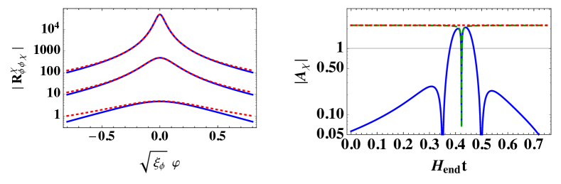
Figure 13: Left: The magnitude of the Riemann spike as a function of the rescaled background field $\sqrt{\xi_{\phi}}\varphi$ for $\xi_{\phi}=1,10,100$ (bottom to top) and $\xi_{\chi}=0.8\xi_{\phi}$. The blue line shows the exact result and the dashed red line the Lorentzian approximation. Right: The adiabaticity parameter for $\xi_{\phi}=100$, $\xi_{\chi}=80$ around the first inflaton zero-crossing for $k\to 0$. The blue curve shows the full result and the green-dotted shows the result of only considering the Riemann term of the effective mass. The red-dotted line shows the analytic result $2/\sqrt{1-\varepsilon}$.

Fig. 14 shows both the Riemann term of the effective mass as well as the (numerically computed) adiabaticity parameter for three values of $\xi_{\chi}$, corresponding to three different values of the ellipticity $\varepsilon=\pm 0.5$ and $\varepsilon=0.2$. We see that our analytic estimates are in line with the numerical result, and, more importantly, we see that decreasing the value of the ellipticity $\varepsilon$ increases the height of the Riemann spike but reduces the maximum value of the adiabaticity parameter. The corresponding values of the effective mass $m^{2}_{\text{eff},\chi}$ are shown in the right panel of Fig. 15.

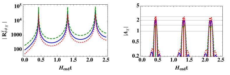
Figure 14: Left: The magnitude of the Riemann spike for $\xi_{\phi}=100$ and $\varepsilon=0.2,-0.5,0.5$ (blue, dashed green, dotted red, respectively). Right: The adiabaticity parameter for the same parameters and color-coding.

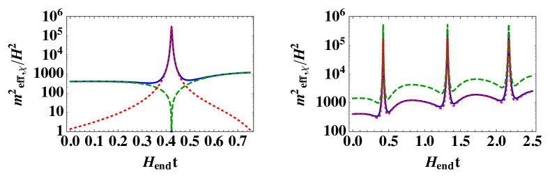
Figure 15: Left: Contributions to the effective mass $m^{2}_{\text{eff},\chi}$ for $\xi_{\phi}=100$ and $\xi_{\chi}=80$ (Case A). The full mass rescaled by the Hubble parameter is shown in blue, $m^{2}_{1,\chi}/H^{2}$ in dashed green and $m^{2}_{2,\chi}/H^{2}$ in dotted red. The contribution of the spacetime Ricci scalar is suppressed and hence is not visible in the graph. Right: The effective mass $m^{2}_{\text{eff},\chi}$ for $\xi_{\phi}=100$ and $\varepsilon=0.2,-0.5,0.5$ (blue, dashed green, dotted red, respectively).

Appendix C Comparing Lattice Results with Linearized Analysis: Wavenumber Binning Effects

In order to present the results of our lattice simulations, we collect all independent wavenumbers and bin them in intervals of $\Delta k=2\pi/L$, where $L$ is the comoving size of the lattice. (A related discussion of sampling effects in lattice simulations of field theory systems related to preheating can be found in Ref. Adshead et al. (2016).) For a three-dimensional lattice of (comoving) size $L$, the corresponding wavenumbers are

$$\vec{k}={2\pi\over L}(\pm n,\pm m,\pm l)\,,$$ (54)

where $n,m,l$ are positive integers bounded from above by the total number of grid points in each direction, which is equal to $L/\Delta x$, where $\Delta x$ is the (comoving) grid spacing. The number $N$ of independent modes in each bin $k$ scales as $k\sim N^{2}$ for low $k$, until the magnitude of the wavenumber reaches $k=k_{\rm max}/2$ at which point the number of modes in each bin begins to decrease (related to the Nyquist frequency). This scaling is simply the density of states in a spherical shell in three dimensions. By choosing the amplitude and phases of the initial conditions of each mode from Gaussian distributions, the resulting power spectra exhibit a variation of $1/\sqrt{N}$. In order to reduce the statistical variance in the final spectra, we bin neighboring wavenumbers by adding squared amplitudes of the various wavenumbers that fit in each bin. Each bin is labeled by the lowest integer wavenumber it contains, so that the $k=10\,H_{\rm end}$ bin actually contains wavenumbers $10\lesssim k/H_{\rm end}\lesssim 12$. As a simple way to properly compare with the lattice results, we compute the following weighted average for the mode $k=10H_{\rm end}$

$$|Q_{{k=10H_{\rm end}}}^{\rm lin.}|^{2}={1\over 10^{2}+11^{2}+12^{2}}\left(10^{2}|Q_{k=10H_{\rm end}}|^{2}+11^{2}|Q_{k=11H_{\rm end}}|^{2}+12^{2}|Q_{k=12H_{\rm end}}|^{2}\right)\,,$$ (55)

with obvious generalization for any wavenumber $k$.

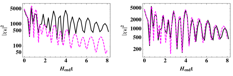
Figure 16: Comparison of the binned lattice results (black) to the linearized fluctuation analysis (dashed magenta) for the case of positive ellipticity with $\xi_{\chi}=0.5\xi_{\phi}$ for $\xi_{\phi}=10$ and $k=10\,H_{\rm end}$. On the left, the linear result is shown only using the mode $k=10\,H_{\rm end}$, whereas on the right, the linear result is computed using the weighted average of binned modes according to Eq. (55).

We see in Fig. 16 that by using the weighted average procedure of Eq. (55) we find excellent agreement between results of the lattice simulations and a linearized analysis (to first order in fluctuations $\delta\phi^{I}$), as long as the fluctuations have not entered the nonlinear regime. Note that for lower values of $k$, fewer wavenumbers are included in each bin, hence it is more likely to observe large statistical variations in the lattice results.

Appendix D Excited Wavenumbers and Numerical Convergence Tests

In this Appendix we consider various requirements on lattice size and other simulation parameters. In order for a lattice simulation to capture relevant dynamics during preheating, the lattice size should be comparable to the Hubble horizon at the end of inflation, hence $k_{\rm min}\lesssim H_{\rm end}$, where $k_{\rm min}$ is the smallest comoving wavenumber in our spectrum (corresponding to the longest wavelength). Meanwhile, for typical values of the couplings, one can show that the modes with comoving wavenumber up to $k_{\rm max}\sim\sqrt{\lambda_{\phi}}\,M_{\rm pl}$ are typically subject to parametric amplification in this family of models DeCross et al. (2018b, c); Ema et al. (2017); Sfakianakis and van de Vis (2019). During inflation in these models, moreover, the Hubble scale behaves as $H^{2}\simeq\lambda_{\phi}\,M_{\rm pl}^{2}/(12\xi_{\phi}^{2})$, so we have

$${k_{\rm max}\over H_{\rm end}}={\cal O}(1)\,\xi_{\phi}\,.$$ (56)

In order for a lattice simulation to accurately capture all relevant dynamics of preheating in this family of models, we therefore require ${\cal O}(\xi_{\phi})$ grid points in each spatial direction. Thus simulations with $\xi_{\phi}>100$ become increasingly expensive.

A further consideration concerns the possible contribution of unphysical ultraviolet (UV) modes to the system’s dynamics. Physically, modes that are not excited above the (local adiabatic) vacuum state should not affect the dynamics of the system. Yet classical simulations are based on seeding all modes within the lattice, with initial amplitudes set by the Bunch-Davies (or WKB) values, and then allowing all of the modes to evolve and interact with each other. This can lead to numerical artifacts arising from unphysical contributions from vacuum UV modes. In order to eliminate such contamination in a controlled way, we introduce an initial suppression of the power in small-wavelength modes by multiplying the initial power spectrum by a window function in momentum space of the form

$$F(k)=\frac{1}{2}\left[1-{\rm tanh}\left(s\left(k-k_{\rm UV}\right)\right)\right]\,,$$ (57)

where $s$ controls the sharpness of the transition between suppressed and unsuppressed regions of the initial power spectrum, and $k_{\rm UV}$ is the (comoving) threshold wavenumber above which initial power is suppressed. Throughout the main body of this paper, we used $k_{\rm UV}=50\,H_{\rm end}$.

To test the robustness of our numerical results, we performed additional simulations with $k_{\rm UV}/H_{\rm end}=25,50,100$. For small and intermediate values of the nonminimal couplings ($\xi_{\phi}=1,10$), we found that the late-time results were entirely independent of $k_{\rm UV}$, as expected, since in these cases both the linearized analysis DeCross et al. (2018a, b, c) and our lattice simulations showed significantly weaker parameter amplification than the case with large nonminimal couplings ($\xi_{\phi}=100$). For $\xi_{\phi}=100$, we found that the early-time behavior of the variances of the $\phi$ and $\chi$ fields depended on the choice of $k_{\rm UV}$, but that the late-time behavior of each field was essentially independent of $k_{\rm UV}$, as shown in Fig. 17.

We can analyze the effect of varying $k_{\rm UV}$ for $\xi_{\phi}=100$ in more detail. For the $\delta\phi$ fluctuations, since no significant parametric resonance is present at early times, increasing $k_{\rm UV}$ simply increases the number of modes that contribute to the initial value of $\langle\phi^{2}\rangle$. Since these higher-$k$ modes remain in the vacuum state, their contribution would be removed via renormalization in a fully quantum-mechanical calculation, which is not possible in a (classical) lattice simulation. Nonetheless, we see that the impact of varying $k_{\rm UV}$ vanishes after the first two oscillations of the inflaton condensate (that is, by the third zero-crossing of $\langle\phi\rangle$), after which backreaction and mode-mode interactions dominate the dynamics. For the $\delta\chi$ fluctuations, we find some amplification of modes with large $k$ at early times, and hence some dependence of the early-time field variance on $k_{\rm UV}$. However, just as for the $\phi$ field, by the second oscillation of the inflaton condensate the variance of $\chi$ becomes essentially independent of $k_{\rm UV}$.

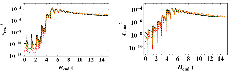
Figure 17: The variance of the $\phi$ field (left) and the $\chi$ field (right) for the benchmark Case A with $\xi_{\phi}=100$ and various values of the initial UV suppression scale $k_{\rm UV}/H_{\rm end}=25,50,100$ (dotted red, dashed green, and dashed black). The late-time behavior of each field is independent of our choice of $k_{\rm UV}$. The orange-dotted curves show the results of a run with ${\cal N}=512^{3}$ grid points (rather than ${\cal N}=256^{3}$) and $k_{\rm UV}/H_{\rm end}=50$, again showing excellent agreement between the various simulations.

In sum, at late times, when nonlinear interactions dominate, both the $\phi$ and $\chi$ spectra are independent of the choice of $k_{\rm UV}$. In particular, the nonlinear dynamics generate a strong cascade of power toward higher-$k$ modes, yielding a smooth final spectrum for each field, which exhibits no memory of the initial window function or the value of $k_{\rm UV}$ that had been used.

Likewise, we find very little dependence of our numerical results as we vary the number of grid points ${\cal N}$, as shown in Fig. 17. If we keep the UV suppression scale fixed at $k_{\rm UV}=50\,H_{\rm end}$ and change from ${\cal N}=256^{3}$ to $512^{3}$, the behavior of the system is essentially indistinguishable for times through $H_{\rm end}\,t\simeq 6$, which is when preheating completes for this set of couplings. After that time, the results of the two simulations track each other well, though the simulation with ${\cal N}=512^{3}$ exhibits more visible oscillations in the variances of each field. This is related to the strong cascade of power toward higher-$k$ modes: the increased number of grid points allows us to capture a larger part of this UV cascade. However, this very slight difference at late times has no effect on the physical quantities of interest, such as duration of reheating $N_{\rm reh}$ or the effective equation of state. For smaller values of $\xi_{\phi}$, for which the UV cascade is weaker, the late-time results show even less variation with ${\cal N}$.

Finally, it is worth noting that the problem studied here is well within the the regime in which a semiclassical approximation is valid. In all of the cases in which these nonperturbative effects occur, the system we study is within the region of validity of a classical, real-time treatment (e.g., exhibiting large occupation numbers), as originally discussed in Refs. Khlebnikov and Tkachev (1996); Prokopec and Roos (1997). A detailed description of contemporary lattice methods can be found in Ref. Figueroa et al. (2020).

References

- Guth et al. (2014) Alan H. Guth, David I. Kaiser, and Yasunori Nomura, “Inflationary paradigm after Planck 2013,” Phys. Lett. B 733, 112–119 (2014), arXiv:1312.7619 [astro-ph.CO] .
- Martin (2016) Jerome Martin, “The Observational Status of Cosmic Inflation after Planck,” The Cosmic Microwave Background, Astrophys. Space Sci. Proc. 45, 41–134 (2016), arXiv:1502.05733 [astro-ph.CO] .
- Chowdhury et al. (2019) Debika Chowdhury, Jérôme Martin, Christophe Ringeval, and Vincent Vennin, “Assessing the scientific status of inflation after Planck,” Phys. Rev. D 100, 083537 (2019), arXiv:1902.03951 [astro-ph.CO] .
- Martin and Ringeval (2010) Jerome Martin and Christophe Ringeval, “First CMB Constraints on the Inflationary Reheating Temperature,” Phys. Rev. D82, 023511 (2010), arXiv:1004.5525 [astro-ph.CO] .
- Mielczarek (2011) Jakub Mielczarek, “Reheating temperature from the CMB,” Phys. Rev. D83, 023502 (2011), arXiv:1009.2359 [astro-ph.CO] .
- Martin et al. (2015) Jerome Martin, Christophe Ringeval, and Vincent Vennin, “Observing Inflationary Reheating,” Phys. Rev. Lett. 114, 081303 (2015), arXiv:1410.7958 [astro-ph.CO] .
- Munoz and Kamionkowski (2015) Julian B. Munoz and Marc Kamionkowski, “Equation-of-State Parameter for Reheating,” Phys. Rev. D91, 043521 (2015), arXiv:1412.0656 [astro-ph.CO] .
- Creminelli et al. (2014a) Paolo Creminelli, Diana López Nacir, Marko Simonović, Gabriele Trevisan, and Matias Zaldarriaga, “ or Not : Testing the Simplest Inflationary Potential,” Phys. Rev. Lett. 112, 241303 (2014a), arXiv:1404.1065 [astro-ph.CO] .
- Creminelli et al. (2014b) Paolo Creminelli, Diana López Nacir, Marko Simonović, Gabriele Trevisan, and Matias Zaldarriaga, “ Inflation at its Endpoint,” Phys. Rev. D90, 083513 (2014b), arXiv:1405.6264 [astro-ph.CO] .
- Dai et al. (2014) Liang Dai, Marc Kamionkowski, and Junpu Wang, “Reheating constraints to inflationary models,” Phys. Rev. Lett. 113, 041302 (2014), arXiv:1404.6704 [astro-ph.CO] .
- Cai et al. (2015) Rong-Gen Cai, Zong-Kuan Guo, and Shao-Jiang Wang, “Reheating phase diagram for single-field slow-roll inflationary models,” Phys. Rev. D92, 063506 (2015), arXiv:1501.07743 [gr-qc] .
- Cook et al. (2015) Jessica L. Cook, Emanuela Dimastrogiovanni, Damien A. Easson, and Lawrence M. Krauss, “Reheating predictions in single field inflation,” JCAP 1504, 047 (2015), arXiv:1502.04673 [astro-ph.CO] .
- Eshaghi et al. (2016) Mehdi Eshaghi, Moslem Zarei, Nematollah Riazi, and Ahmad Kiasatpour, “CMB and reheating constraints to -attractor inflationary models,” Phys. Rev. D93, 123517 (2016), arXiv:1602.07914 [astro-ph.CO] .
- Ueno and Yamamoto (2016) Yoshiki Ueno and Kazuhiro Yamamoto, “Constraints on -attractor inflation and reheating,” Phys. Rev. D93, 083524 (2016), arXiv:1602.07427 [astro-ph.CO] .
- Figueroa and Tanin (2019) Daniel G. Figueroa and Erwin H. Tanin, “Inconsistency of an inflationary sector coupled only to Einstein gravity,” JCAP 1910, 050 (2019), arXiv:1811.04093 [astro-ph.CO] .
- Amin (2010) Mustafa A. Amin, “Inflaton fragmentation: Emergence of pseudo-stable inflaton lumps (oscillons) after inflation,” (2010), arXiv:1006.3075 [astro-ph.CO] .
- Amin et al. (2010) Mustafa A. Amin, Richard Easther, and Hal Finkel, “Inflaton Fragmentation and Oscillon Formation in Three Dimensions,” JCAP 1012, 001 (2010), arXiv:1009.2505 [astro-ph.CO] .
- Gleiser et al. (2011) Marcelo Gleiser, Noah Graham, and Nikitas Stamatopoulos, “Generation of Coherent Structures After Cosmic Inflation,” Phys. Rev. D83, 096010 (2011), arXiv:1103.1911 [hep-th] .
- Amin et al. (2012) Mustafa A. Amin, Richard Easther, Hal Finkel, Raphael Flauger, and Mark P. Hertzberg, “Oscillons After Inflation,” Phys. Rev. Lett. 108, 241302 (2012), arXiv:1106.3335 [astro-ph.CO] .
- Lozanov and Amin (2018) Kaloian D. Lozanov and Mustafa A. Amin, “Self-resonance after inflation: oscillons, transients and radiation domination,” Phys. Rev. D97, 023533 (2018), arXiv:1710.06851 [astro-ph.CO] .
- Hong et al. (2018) Jeong-Pyong Hong, Masahiro Kawasaki, and Masahito Yamazaki, “Oscillons from Pure Natural Inflation,” Phys. Rev. D98, 043531 (2018), arXiv:1711.10496 [astro-ph.CO] .
- Fukunaga et al. (2019) Hayato Fukunaga, Naoya Kitajima, and Yuko Urakawa, “Efficient self-resonance instability from axions,” JCAP 1906, 055 (2019), arXiv:1903.02119 [astro-ph.CO] .
- Bassett et al. (2006) Bruce A. Bassett, Shinji Tsujikawa, and David Wands, “Inflation dynamics and reheating,” Rev. Mod. Phys. 78, 537–589 (2006), arXiv:astro-ph/0507632 [astro-ph] .
- Frolov (2010) Andrei V. Frolov, “Non-linear Dynamics and Primordial Curvature Perturbations from Preheating,” Class. Quant. Grav. 27, 124006 (2010), arXiv:1004.3559 [gr-qc] .
- Allahverdi et al. (2010) Rouzbeh Allahverdi, Robert Brandenberger, Francis-Yan Cyr-Racine, and Anupam Mazumdar, “Reheating in Inflationary Cosmology: Theory and Applications,” Ann. Rev. Nucl. Part. Sci. 60, 27–51 (2010), arXiv:1001.2600 [hep-th] .
- Amin et al. (2014) Mustafa A. Amin, Mark P. Hertzberg, David I. Kaiser, and Johanna Karouby, “Nonperturbative Dynamics Of Reheating After Inflation: A Review,” Int. J. Mod. Phys. D24, 1530003 (2014), arXiv:1410.3808 [hep-ph] .
- Lozanov (2019) Kaloian D. Lozanov, “Lectures on Reheating after Inflation,” (2019), arXiv:1907.04402 [astro-ph.CO] .
- Callan et al. (1970) Jr. Callan, Curtis G., Sidney R. Coleman, and Roman Jackiw, “A New improved energy - momentum tensor,” Annals Phys. 59, 42–73 (1970).
- Bunch et al. (1980) T.S. Bunch, P. Panangaden, and L. Parker, “On renormalization of field theory in curved space-time, I,” J. Phys. A 13, 901–918 (1980).
- Bunch and Panangaden (1980) T.S. Bunch and P. Panangaden, “On renormalization of field theory in curved space-time, II,” J. Phys. A 13, 919–932 (1980).
- Birrell and Davies (1982) N.D. Birrell and P.C.W. Davies, Quantum Fields in Curved Space (Cambridge Univ. Press, Cambridge, UK, 1982).
- Odintsov (1991) Sergei D. Odintsov, “Renormalization Group, Effective Action and Grand Unification Theories in Curved Space-time,” Fortsch. Phys. 39, 621–641 (1991).
- Buchbinder et al. (1992) I.L. Buchbinder, S.D. Odintsov, and I.L. Shapiro, Effective action in quantum gravity (Taylor and Francis, New York, 1992).
- Parker and Toms (2009) Leonard E. Parker and D. Toms, Quantum Field Theory in Curved Spacetime: Quantized Field and Gravity (Cambridge University Press, New York, 2009).
- Markkanen and Tranberg (2013) Tommi Markkanen and Anders Tranberg, “A Simple Method for One-Loop Renormalization in Curved Space-Time,” JCAP 08, 045 (2013), arXiv:1303.0180 [hep-th] .
- Bezrukov and Shaposhnikov (2008) Fedor L. Bezrukov and Mikhail Shaposhnikov, “The Standard Model Higgs boson as the inflaton,” Phys. Lett. B659, 703–706 (2008), arXiv:0710.3755 [hep-th] .
- Greenwood et al. (2013) Ross N. Greenwood, David I. Kaiser, and Evangelos I. Sfakianakis, “Multifield Dynamics of Higgs Inflation,” Phys. Rev. D 87, 064021 (2013), arXiv:1210.8190 [hep-ph] .
- Sfakianakis and van de Vis (2019) Evangelos I. Sfakianakis and Jorinde van de Vis, “Preheating after Higgs Inflation: Self-Resonance and Gauge boson production,” Phys. Rev. D99, 083519 (2019), arXiv:1810.01304 [hep-ph] .
- Ema et al. (2020) Yohei Ema, Kyohei Mukaida, and Jorinde van de Vis, “Higgs Inflation as Nonlinear Sigma Model and Scalaron as its -meson,” (2020), arXiv:2002.11739 [hep-ph] .
- Kaiser and Sfakianakis (2014) David I. Kaiser and Evangelos I. Sfakianakis, “Multifield Inflation after Planck: The Case for Nonminimal Couplings,” Phys. Rev. Lett. 112, 011302 (2014), arXiv:1304.0363 [astro-ph.CO] .
- Kaiser et al. (2013) David I. Kaiser, Edward A. Mazenc, and Evangelos I. Sfakianakis, “Primordial Bispectrum from Multifield Inflation with Nonminimal Couplings,” Phys. Rev. D 87, 064004 (2013), arXiv:1210.7487 [astro-ph.CO] .
- Schutz et al. (2014) Katelin Schutz, Evangelos I. Sfakianakis, and David I. Kaiser, “Multifield Inflation after Planck: Isocurvature Modes from Nonminimal Couplings,” Phys. Rev. D 89, 064044 (2014), arXiv:1310.8285 [astro-ph.CO] .
- Nguyen et al. (2019) Rachel Nguyen, Jorinde van de Vis, Evangelos I. Sfakianakis, John T. Giblin, and David I. Kaiser, “Nonlinear Dynamics of Preheating after Multifield Inflation with Nonminimal Couplings,” Phys. Rev. Lett. 123, 171301 (2019), arXiv:1905.12562 [hep-ph] .
- DeCross et al. (2018a) Matthew P. DeCross, David I. Kaiser, Anirudh Prabhu, C. Prescod-Weinstein, and Evangelos I. Sfakianakis, “Preheating after Multifield Inflation with Nonminimal Couplings, I: Covariant Formalism and Attractor Behavior,” Phys. Rev. D 97, 023526 (2018a), arXiv:1510.08553 [astro-ph.CO] .
- DeCross et al. (2018b) Matthew P. DeCross, David I. Kaiser, Anirudh Prabhu, Chanda Prescod-Weinstein, and Evangelos I. Sfakianakis, “Preheating after multifield inflation with nonminimal couplings, II: Resonance Structure,” Phys. Rev. D 97, 023527 (2018b), arXiv:1610.08868 [astro-ph.CO] .
- DeCross et al. (2018c) Matthew P. DeCross, David I. Kaiser, Anirudh Prabhu, Chanda Prescod-Weinstein, and Evangelos I. Sfakianakis, “Preheating after multifield inflation with nonminimal couplings, III: Dynamical spacetime results,” Phys. Rev. D 97, 023528 (2018c), arXiv:1610.08916 [astro-ph.CO] .
- Kaiser (2010) David I. Kaiser, “Conformal Transformations with Multiple Scalar Fields,” Phys. Rev. D 81, 084044 (2010), arXiv:1003.1159 [gr-qc] .
- Abedi and Abbassi (2015) Habib Abedi and Amir M. Abbassi, “Gravitational constant in multiple field gravity,” JCAP 05, 026 (2015), arXiv:1411.4854 [gr-qc] .
- Gong and Tanaka (2011) Jinn-Ouk Gong and Takahiro Tanaka, “A covariant approach to general field space metric in multi-field inflation,” JCAP 03, 015 (2011), [Erratum: JCAP 02, E01 (2012)], arXiv:1101.4809 [astro-ph.CO] .
- Gong (2016) Jinn-Ouk Gong, “Multi-field inflation and cosmological perturbations,” Int. J. Mod. Phys. D 26, 1740003 (2016), arXiv:1606.06971 [gr-qc] .
- Ema et al. (2017) Yohei Ema, Ryusuke Jinno, Kyohei Mukaida, and Kazunori Nakayama, “Violent Preheating in Inflation with Nonminimal Coupling,” JCAP 1702, 045 (2017), arXiv:1609.05209 [hep-ph] .
- Kwapisz and Meissner (2018) Jan Kwapisz and Krzysztof A. Meissner, “Conformal Standard Model and Inflation,” Acta Phys. Polon. B 49, 115 (2018), arXiv:1712.03778 [gr-qc] .
- Akrami et al. (2018) Y. Akrami et al. (Planck), “Planck 2018 results. X. Constraints on inflation,” (2018), arXiv:1807.06211 [astro-ph.CO] .
- Bezrukov and Gorbunov (2013) F. Bezrukov and D. Gorbunov, “Light inflaton after LHC8 and WMAP9 results,” JHEP 07, 140 (2013), arXiv:1303.4395 [hep-ph] .
- Barvinsky et al. (2012) A.O. Barvinsky, A.Yu. Kamenshchik, C. Kiefer, A.A. Starobinsky, and C.F. Steinwachs, “Higgs boson, renormalization group, and naturalness in cosmology,” Eur. Phys. J. C 72, 2219 (2012), arXiv:0910.1041 [hep-ph] .
- Barvinsky et al. (2009) A.O. Barvinsky, A.Yu. Kamenshchik, C. Kiefer, A.A. Starobinsky, and C. Steinwachs, “Asymptotic freedom in inflationary cosmology with a non-minimally coupled Higgs field,” JCAP 12, 003 (2009), arXiv:0904.1698 [hep-ph] .
- Bezrukov et al. (2012) Fedor Bezrukov, Mikhail Yu. Kalmykov, Bernd A. Kniehl, and Mikhail Shaposhnikov, “Higgs Boson Mass and New Physics,” JHEP 10, 140 (2012), arXiv:1205.2893 [hep-ph] .
- Allison (2014) Kyle Allison, “Higgs -inflation for the 125-126 GeV Higgs: a two-loop analysis,” JHEP 02, 040 (2014), arXiv:1306.6931 [hep-ph] .
- Giblin and Tishue (2019) John T. Giblin and Avery J. Tishue, “Preheating in Full General Relativity,” Phys. Rev. D100, 063543 (2019), arXiv:1907.10601 [gr-qc] .
- Giblin et al. (2019) John T. Giblin, James B. Mertens, Glenn D. Starkman, and Chi Tian, “Limited accuracy of linearized gravity,” Phys. Rev. D99, 023527 (2019), arXiv:1810.05203 [astro-ph.CO] .
- Wands (2008) David Wands, “Multiple field inflation,” Lect. Notes Phys. 738, 275–304 (2008), arXiv:astro-ph/0702187 .
- Langlois and Renaux-Petel (2008) David Langlois and Sebastien Renaux-Petel, “Perturbations in generalized multi-field inflation,” JCAP 04, 017 (2008), arXiv:0801.1085 [hep-th] .
- Renaux-Petel and Turzyński (2016) Sébastien Renaux-Petel and Krzysztof Turzyński, “Geometrical Destabilization of Inflation,” Phys. Rev. Lett. 117, 141301 (2016), arXiv:1510.01281 [astro-ph.CO] .
- (64) http://cosmo.kenyon.edu/gabe.html.
- Child et al. (2013) Hillary L. Child, John T. Giblin, Jr, Raquel H. Ribeiro, and David Seery, “Preheating with Non-Minimal Kinetic Terms,” Phys. Rev. Lett. 111, 051301 (2013), arXiv:1305.0561 [astro-ph.CO] .
- Bassett et al. (1999a) Bruce A. Bassett, David I. Kaiser, and Roy Maartens, “General relativistic preheating after inflation,” Phys. Lett. B 455, 84–89 (1999a), arXiv:hep-ph/9808404 .
- Bassett et al. (1999b) Bruce A. Bassett, Fabrizio Tamburini, David I. Kaiser, and Roy Maartens, “Metric preheating and limitations of linearized gravity. 2.” Nucl. Phys. B 561, 188–240 (1999b), arXiv:hep-ph/9901319 .
- Bassett et al. (2000) Bruce A. Bassett, Christopher Gordon, Roy Maartens, and David I. Kaiser, “Restoring the sting to metric preheating,” Phys. Rev. D 61, 061302 (2000), arXiv:hep-ph/9909482 .
- Gordon et al. (2000) Christopher Gordon, David Wands, Bruce A. Bassett, and Roy Maartens, “Adiabatic and entropy perturbations from inflation,” Phys. Rev. D 63, 023506 (2000), arXiv:astro-ph/0009131 .
- Elliston et al. (2011) Joseph Elliston, David J. Mulryne, David Seery, and Reza Tavakol, “Evolution of to the adiabatic limit,” JCAP 11, 005 (2011), arXiv:1106.2153 [astro-ph.CO] .
- Meyers and Tarrant (2014) Joel Meyers and Ewan R. M. Tarrant, “Perturbative Reheating After Multiple-Field Inflation: The Impact on Primordial Observables,” Phys. Rev. D 89, 063535 (2014), arXiv:1311.3972 [astro-ph.CO] .
- Elliston et al. (2014) Joseph Elliston, Stefano Orani, and David J. Mulryne, “General analytic predictions of two-field inflation and perturbative reheating,” Phys. Rev. D 89, 103532 (2014), arXiv:1402.4800 [astro-ph.CO] .
- Renaux-Petel and Turzynski (2015) Sebastien Renaux-Petel and Krzysztof Turzynski, “On reaching the adiabatic limit in multi-field inflation,” JCAP 06, 010 (2015), arXiv:1405.6195 [astro-ph.CO] .
- Micha and Tkachev (2003) Raphael Micha and Igor I. Tkachev, “Relativistic turbulence: A Long way from preheating to equilibrium,” Phys. Rev. Lett. 90, 121301 (2003), arXiv:hep-ph/0210202 .
- Micha and Tkachev (2004) Raphael Micha and Igor I. Tkachev, “Turbulent thermalization,” Phys. Rev. D 70, 043538 (2004), arXiv:hep-ph/0403101 .
- McDonough (2020) Evan McDonough, “The Cosmological Heavy Ion Collider: Fast Thermalization after Cosmic Inflation,” (2020), arXiv:2001.03633 [hep-th] .
- Bezrukov et al. (2009) F. Bezrukov, D. Gorbunov, and M. Shaposhnikov, “On initial conditions for the Hot Big Bang,” JCAP 06, 029 (2009), arXiv:0812.3622 [hep-ph] .
- Garcia-Bellido et al. (2009) Juan Garcia-Bellido, Daniel G. Figueroa, and Javier Rubio, “Preheating in the Standard Model with the Higgs-Inflaton coupled to gravity,” Phys. Rev. D 79, 063531 (2009), arXiv:0812.4624 [hep-ph] .
- Dufaux et al. (2010) Jean-Francois Dufaux, Daniel G. Figueroa, and Juan Garcia-Bellido, “Gravitational Waves from Abelian Gauge Fields and Cosmic Strings at Preheating,” Phys. Rev. D 82, 083518 (2010), arXiv:1006.0217 [astro-ph.CO] .
- Repond and Rubio (2016) Jo Repond and Javier Rubio, “Combined Preheating on the lattice with applications to Higgs inflation,” JCAP 07, 043 (2016), arXiv:1604.08238 [astro-ph.CO] .
- Greene and Kofman (1999) Patrick B. Greene and Lev Kofman, “Preheating of fermions,” Phys. Lett. B448, 6–12 (1999), arXiv:hep-ph/9807339 [hep-ph] .
- Greene and Kofman (2000) Patrick B. Greene and Lev Kofman, “On the theory of fermionic preheating,” Phys. Rev. D62, 123516 (2000), arXiv:hep-ph/0003018 [hep-ph] .
- Peloso and Sorbo (2000) Marco Peloso and Lorenzo Sorbo, “Preheating of massive fermions after inflation: Analytical results,” JHEP 0005, 016 (2000), arXiv:hep-ph/0003045 [hep-ph] .
- Tsujikawa et al. (2000) Shinji Tsujikawa, Bruce A. Bassett, and Fermin Viniegra, “Multifield fermionic preheating,” JHEP 08, 019 (2000), arXiv:hep-ph/0006354 [hep-ph] .
- Adshead and Sfakianakis (2015) Peter Adshead and Evangelos I. Sfakianakis, “Fermion production during and after axion inflation,” JCAP 1511, 021 (2015), arXiv:1508.00891 [hep-ph] .
- Adshead et al. (2018a) Peter Adshead, Andrew J. Long, and Evangelos I. Sfakianakis, “Gravitational Leptogenesis, Reheating, and Models of Neutrino Mass,” Phys. Rev. D97, 043511 (2018a), arXiv:1711.04800 [hep-ph] .
- Davis et al. (2001) Anne-Christine Davis, Konstantinos Dimopoulos, Tomislav Prokopec, and Ola Tornkvist, “Primordial spectrum of gauge fields from inflation,” Phys. Lett. B501, 165–172 (2001), arXiv:astro-ph/0007214 [astro-ph] .
- Garcia-Bellido et al. (2004) Juan Garcia-Bellido, Margarita Garcia-Perez, and Antonio Gonzalez-Arroyo, “Chern-Simons production during preheating in hybrid inflation models,” Phys. Rev. D69, 023504 (2004), arXiv:hep-ph/0304285 [hep-ph] .
- Braden et al. (2010) Jonathan Braden, Lev Kofman, and Neil Barnaby, “Reheating the Universe After Multi-Field Inflation,” JCAP 1007, 016 (2010), arXiv:1005.2196 [hep-th] .
- Allahverdi et al. (2011) Rouzbeh Allahverdi, Andrea Ferrantelli, Juan Garcia-Bellido, and Anupam Mazumdar, “Non-perturbative production of matter and rapid thermalization after MSSM inflation,” Phys. Rev. D83, 123507 (2011), arXiv:1103.2123 [hep-ph] .
- Deskins et al. (2013) J. Tate Deskins, John T. Giblin, and Robert R. Caldwell, “Gauge Field Preheating at the End of Inflation,” Phys. Rev. D88, 063530 (2013), arXiv:1305.7226 [astro-ph.CO] .
- Adshead et al. (2015) Peter Adshead, John T. Giblin, Timothy R. Scully, and Evangelos I. Sfakianakis, “Gauge-preheating and the end of axion inflation,” JCAP 1512, 034 (2015), arXiv:1502.06506 [astro-ph.CO] .
- Adshead et al. (2017) Peter Adshead, John T. Giblin, and Zachary J. Weiner, “Non-Abelian gauge preheating,” Phys. Rev. D96, 123512 (2017), arXiv:1708.02944 [hep-ph] .
- Cuissa and Figueroa (2019) Jose Roberto Canivete Cuissa and Daniel G. Figueroa, “Lattice formulation of axion inflation. Application to preheating,” JCAP 1906, 002 (2019), arXiv:1812.03132 [astro-ph.CO] .
- Adshead et al. (2018b) Peter Adshead, John T. Giblin, and Zachary J. Weiner, “Gravitational waves from gauge preheating,” Phys. Rev. D98, 043525 (2018b), arXiv:1805.04550 [astro-ph.CO] .
- Lozanov and Amin (2019) Kaloian D. Lozanov and Mustafa A. Amin, “Gravitational perturbations from oscillons and transients after inflation,” Phys. Rev. D99, 123504 (2019), arXiv:1902.06736 [astro-ph.CO] .
- Christodoulidis et al. (2019a) Perseas Christodoulidis, Diederik Roest, and Evangelos I. Sfakianakis, “Scaling attractors in multi-field inflation,” JCAP 12, 059 (2019a), arXiv:1903.06116 [hep-th] .
- Christodoulidis et al. (2019b) Perseas Christodoulidis, Diederik Roest, and Evangelos I. Sfakianakis, “Attractors, Bifurcations and Curvature in Multi-field Inflation,” (2019b), arXiv:1903.03513 [gr-qc] .
- Iarygina et al. (2020) Oksana Iarygina, Evangelos I. Sfakianakis, Dong-Gang Wang, and Ana Achúcarro, “Multi-field inflation and preheating in asymmetric -attractors,” (2020), arXiv:2005.00528 [astro-ph.CO] .
- Adshead et al. (2016) Peter Adshead, John T. Giblin, Timothy R. Scully, and Evangelos I. Sfakianakis, “Magnetogenesis from axion inflation,” JCAP 1610, 039 (2016), arXiv:1606.08474 [astro-ph.CO] .
- Khlebnikov and Tkachev (1996) S.Yu. Khlebnikov and I.I. Tkachev, “Classical decay of inflaton,” Phys. Rev. Lett. 77, 219–222 (1996), arXiv:hep-ph/9603378 .
- Prokopec and Roos (1997) Tomislav Prokopec and Thomas G. Roos, “Lattice study of classical inflaton decay,” Phys. Rev. D 55, 3768–3775 (1997), arXiv:hep-ph/9610400 .
- Figueroa et al. (2020) Daniel G. Figueroa, Adrien Florio, Francisco Torrenti, and Wessel Valkenburg, “The art of simulating the early Universe – Part I,” (2020), arXiv:2006.15122 [astro-ph.CO] .