]Published 9 November 2020. DOI: 10.1103/PhysRevLett.125.20060

Freezing Transition in the Barrier Crossing Rate of a Diffusing Particle

Abstract

We study the decay rate $\theta(a)$ that characterizes the late time exponential decay of the first-passage probability density $F_{a}(t|0)\sim e^{-\theta(a)\,t}$ of a diffusing particle in a one dimensional confining potential $U(x)$, starting from the origin, to a position located at $a>0$. For general confining potential $U(x)$ we show that $\theta(a)$, a measure of the barrier (located at $a$) crossing rate, has three distinct behaviors as a function of $a$, depending on the tail of $U(x)$ as $x\to-\infty$. In particular, for potentials behaving as $U(x)\sim|x|$ when $x\to-\infty$, we show that a novel freezing transition occurs at a critical value $a=a_{c}$, i.e, $\theta(a)$ increases monotonically as $a$ decreases till $a_{c}$, and for $a\leq a_{c}$ it freezes to $\theta(a)=\theta(a_{c})$. Our results are established using a general mapping to a quantum problem and by exact solution in three representative cases, supported by numerical simulations. We show that the freezing transition occurs when in the associated quantum problem, the gap between the ground state (bound) and the continuum of scattering states vanishes.

Consider an overdamped Brownian particle on a line in the presence of an external potential $U(x)$, whose position $x(t)$ evolves by the Langevin equation

$$\frac{dx}{dt}=-\frac{1}{\Gamma}\,U^{\prime}(x)+\sqrt{2D}\,\eta(t),$$ (1)

where $D=k_{B}T/\Gamma$, with $k_{B}$, $T$, and $\Gamma$ being the Boltzmann constant, temperature and the friction coefficient respectively. The white noise $\eta(t)$ has zero mean and is $\delta$ correlated: $\langle\eta(t)\rangle=0$ and $\langle\eta(t)\eta(t^{\prime})=\delta(t-t^{\prime})$. For a particle starting at a local minimum $x_{0}$ of the potential $U(x)$, what is the rate $\kappa(a)$ with which the particle crosses over a barrier of relative height $\Delta U=U(a)-U(x_{0})$, located at $a>x_{0}$? Estimating $\kappa(a)$ is one of the most important and celebrated problems in the theory of reaction kinetics, often known as Kramers problem. It has found immense applications in physics, chemistry, biology and engineering sciences (for a review with nice historical aspects see HTB1990 ). Assuming near-equilibrium position distribution inside the potential well, the escape rate can be estimated by computing the flux across the barrier Farkas1927 ; KS1934 ; BD1935 ; Kramers1940 ; vanKampen ; HTB1990 . In the low temperature and/or large barrier limit, it is well approximated by the van’t Hoff-Arrhenius form Hoff1884 ; Arrhenius1889 $\kappa(a)\sim e^{-\Delta U/(k_{B}T)}.$

Another alternative approach PAV1933 , that even predates Kramers, consists in estimating $1/\kappa(a)$ by the mean first-passage time $T_{a}(x_{0})$ from $x_{0}$ to $a$. A quantity that carries more information is the full distribution $F_{a}(t|x_{0})$ of the first-passage time to level $a$ starting at $x_{0}$. Evidently, $T_{a}(x_{0})$ is just the first moment of the distribution. The cumulative first-passage distribution $S_{a}(t|x_{0})=\int_{t}^{\infty}F_{a}(t^{\prime}|x_{0})\,dt^{\prime}$ is known as the survival probability, which can in principle be computed by solving the Fokker-Planck equation for the probability density with an absorbing boundary condition at $x=a$ Risken1984 ; SM1999 ; Redner2001 ; SM2005 ; BMS2013 . For a confining potential $U(x)$, usually the Fokker-Planck operator has a discrete spectra, and hence the survival probability [and consequently the first-passage probability] is expected to decay exponentially at late times: $S_{a}(t|x_{0})\sim e^{-\theta(a)\,t}$ where the decay rate $\theta(a)$ gives another estimate of the escape rate $\kappa(a)$. While the mean first-passage time $T_{a}(x_{0})$ can be computed explicitly for arbitrary potential $U(x)$ Risken1984 , the decay rate $\theta(a)$ is much harder to compute and there is no known formula for $\theta(a)$ for general potential $U(x)$, though there has been recent progress for specific cases GM2016a ; HG2018 ; HG2019 ; HG20192 ; MKC2019 .

We remark that even though the problem is posed here in the language of barrier crossing, the first-passage probability of a diffusing particle in a confining potential has a much broader applicability ranging from search processes in animal foraging for food BLMV2011 ; VDRS2011 , all the way to gene transcription regulation GM2016b . For example, in the context of foraging, an animal is typically confined in its home range and searches for a target (food) located at a distance $a$ (from its nest) which need not be always large, as in the Kramers problem. Hence, estimating $\theta(a)$ for all $a$ is a fundamental problem of broad interest.

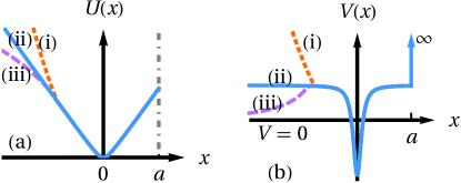
Figure 1: (a) A schematic illustration of classical potentials $U(x)$ whose left tails as $x\to-\infty$, increase (i) faster than $|x|$ (red dotted line), (ii) as $|x|$ (blue solid line), and (iii) slower than $|x|$ (magenta dashed line). There is an absorbing barrier at $x=a$ (dot-dashed line). (b) Schematic illustrations of the corresponding quantum potentials $V(x)$ in Eq. (3), whose left tails as $x\to-\infty$, (i) diverges (red dotted line), (ii) approaches a constant (blue solid line), and (iii) tends to zero (magenta dashed line) respectively. $V(x)=\infty$ for $x\geq a$.

For large $a$, the three estimates of $\kappa(a)$, namely, the Kramers estimate, the inverse mean first-passage time $1/T_{a}(x_{0})$, and the decay rate $\theta(a)$, all have the Arrhenius form $\sim e^{-U(a)/(k_{B}T)}$ [see HG20192 for a more refined estimate of $\theta(a)$ for large $a$]. However, in many search processes discussed above, the location $a$ of the barrier (or the target) is not necessarily large and the three measures may have different $a$ dependences, in particular for small $a$. Indeed, the discrepancy between the last two measures for small $a$ is expected for compact diffusion GM2016b , which is the case here since the potential is confining. In this Letter, we study the $a$ dependence of the three measures for general potential $U(x)$ and show that indeed for small $a$, they are quite different from each other. In particular, we show that $\theta(a)$ for general $U(x)$ displays a rich and robust $a$ dependence, depending on the tail of $U(x)$ as $x\to-\infty$ (see Fig. 1), that is not captured by the other two measures of $\kappa(a)$. More precisely, we find (i) if $U(x)$ increases faster than $|x|$ as $x\to-\infty$, then $\theta(a)$ increases monotonically as $a$ decreases, (ii) if $U(x)\sim|x|$ as $x\to-\infty$, then there is a critical value of $a$ at $a=a_{c}$, where a novel freezing transition occurs, i.e., $\theta(a)$ increases monotonically as $a$ decreases till $a_{c}$, and for $a\leq a_{c}$ the decay rate $\theta(a)=\theta(a_{c})$, and (iii) if $U(x)$ increases slower than $|x|$ as $x\to-\infty$, then $\theta(a)=0$ for all $a$, indicating a slower than exponential decay with time, of the first-passage probability (see Fig. 3).

We establish this behavior by mapping to a quantum problem, where the quantum potential (see Fig. 1) has always bound states in case (i), while in case (iii) it only has a continuous spectrum of scattering states. In the borderline case (ii), the spectrum has a bound state separated by a gap from the continuum of scattering states for $a>a_{c}$, and the gap vanishes as $a\to a_{c}^{+}$ (see Fig. 2). In case (i) and case (ii) with $a>a_{c}$, where the spectrum has bound states, $\theta(a)$ coincides exactly with the ground state energy of the quantum problem. The inverse mean first-passage time $1/T_{a}(x_{0})$, in contrast, always increases monotonically with decreasing $a$, and hence misses this novel freezing transition at $a=a_{c}$ (see Fig. 3). This transition is also consistent with the powerful interlacing theorem derived in HG2018 ; HG2019 ; for details see the Supplemental Material  SM . The mapping to the quantum problem makes it evident that the scenario presented above holds generically for any confining potential $U(x)$. In addition, we show the validity of this generic behavior by explicit exact solution in three representative cases here (for another example, see  SM ).

We start with the Fokker-Planck equation for the probability density function $P(x,t)$ of the particle to be at $x$ at time $t$, without having crossed the level at $x=a$,

$$\frac{\partial P}{\partial t}=D\frac{\partial^{2}P}{\partial x^{2}}+\frac{\partial}{\partial x}\left[U^{\prime}(x)P\right],$$ (2)

where we set $\Gamma=1$ for simplicity. Equation (2) holds in $x\in(-\infty,a)$ with an absorbing boundary condition $P(a,t)=0$ at $x=a$ and also, $P(x\to-\infty,t)=0$. We assume that the particle starts at the origin at $t=0$, i.e., $P(x,0)=\delta(x)$ and the barrier location $a\geq 0$ to be on the right of the initial position of the particle. If $a<0$, one can reverse $x$ and perform a similar analysis. With the transformation Risken1984 , $P(x,t)=e^{-[U(x)-U(0)]/(2D)}\,\psi(x,t),$ Eq. (2) gets mapped to the time-dependent Schrödinger equation in imaginary time, $-\partial\psi/\partial t=\mathcal{H}\psi(x,t),$ where $\mathcal{H}=-D(\partial^{2}/\partial x^{2})+V(x),$ with the initial condition $\psi(x,0)=\delta(x)$ and the quantum potential

$$V(x)=\frac{[U^{\prime}(x)]^{2}}{4D}-\frac{U^{\prime\prime}(x)}{2},\quad\text{for}~{}x<a.$$ (3)

Here we assume $U(x)$ to be twice differentiable almost everywhere. The absorbing boundary condition $P(x=a,t)=0$ translates into $\psi(x=a,t)=0$, which in the quantum problem, corresponds to having an infinite barrier at $x=a$, i.e., $V(x)=\infty$ for $x\geq a$. The wave function $\psi(x,t)$ can be written in the eigenbasis of $\mathcal{H}$, as

$$\psi(x,t)=\sum_{E}\phi_{E}^{*}(0)\,\phi_{E}(x)\,e^{-Et}$$ (4)

where $\mathcal{H}\phi_{E}(x)=E\phi_{E}(x)$, and we have used $\psi(x,0)=\delta(x)$. The sum over $E$ includes both the discrete and the continuous part of the spectrum. When the ground state is bound and is separated by a finite gap from the rest of the spectrum, then it follows from Eq. (4), that at late times $P(x,t)\sim e^{-E_{0}t}$ where $E_{0}$ is the ground state energy. Correspondingly the survival probability $S_{a}(t|0)=\int_{-\infty}^{a}P(x,t)\,dx\sim e^{-\theta(a)\,t}$ with $\theta(a)=E_{0}$.

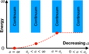
Figure 2: Schematic diagram of energy levels for the quantum potential $V(x)=\alpha^{2}/(4D)-\alpha\delta(x)$ for $x<a$ and $V(x)=\infty$ for $x\geq a$, for different values of $a$. The (red) dots represent the ground state energy for different values of $a$ whereas the (blue) bands represent the continuum of energy levels from $\alpha^{2}/(4D)$ to $\infty$. The gap vanishes at $a=a_{c}=D/\alpha$.

Since there is an infinite barrier at $x=a$, whether the Hamiltonian $\mathcal{H}$ has a bound state or not depends only on the behavior of $V(x)$ as $x\to-\infty$. For example, if the classical potential $U(x)$ increases faster than $|x|$ as $x\to-\infty$ such as $U(x)\sim(-x)^{\gamma}$ with $\gamma>1$, then it is easy to see from Eq. (3) that $V(x)\sim(-x)^{2(\gamma-1)}$, and hence, $V(x)$ diverges as $x\to-\infty$. In this case, clearly, the quantum problem will have only bound states. On the other hand, if $\gamma<1$, then $V(x)\to 0$ as $x\to-\infty$, indicating that the quantum problem will only have scattering states. In the marginal case, $\gamma=1$, $V(x)$ approaches a constant as $x\to-\infty$, and in this case, one would expect that a bound state may or may not exist depending on the value of $a$. To illustrate this general scenario, we present below an exact solution for a representative $U(x)$ whose $x\to-\infty$ tails can be tuned as in the three cases above. More precisely, we choose

$$U(x)=\alpha|x|\quad\text{for}~{}-b<x<a,$$ (5a)

with $$b>0 x<-b$$, and for ,

$$U(x)=\begin{cases}\frac{1}{2}\,\mu x^{2}&\text{for case (i)}\\ \alpha|x|&\text{for case (ii)}\\ c\ln(-x/\lambda)&\text{for case (iii)}\\ \end{cases}$$ (5b)

where $\lambda>0$ is a length scale and for the sake of continuity of the potential at $x=-b$, we set $\mu=2\alpha/b$ and $c\ln(b/\lambda)=\alpha b$ (see Fig. 1).

For convenience, we start our analysis for the marginal case (ii) in Eq. (5b) where $U(x)=\alpha\,|x|$ for $x<a$ and show explicitly that a freezing transition occurs at the critical value $a=a_{c}=D/\alpha$. The cases (i) and (iii) will be discussed subsequently. The quantum potential $V(x)$ from Eq. (3) is then given by $V(x)=\alpha^{2}/(4D)-\alpha\delta(x)$ for $x<a$ and $V(x)=\infty$ for $x\geq a$. In this case, the Schrödinger equation can be solved either by spectral decomposition as in Eq. (4) or equivalently by taking the Laplace transform of the equation with respect to $t$. In the later case, the spectral values of $E$ manifest as poles (for the discrete part of the spectrum) or as a branch cut (for the continuous part of the spectrum). Skipping details (see SM ), the solution in the Laplace space $\tilde{\psi}(x,s)=\int_{0}^{\infty}\psi(x,t)\,e^{-st}\,dt$, reads

$$\tilde{\psi}(x,s)=\begin{cases}\frac{1}{A(p)}\,\bigl{[}1-e^{-pa/D}\bigr{]}\,e^{px/(2D)}&\text{for}~{}x\leq 0,\\[5.69054pt] \frac{1}{A(p)}\,\bigl{[}1-e^{-p(a-x)/D}\bigr{]}\,e^{-px/(2D)}&\text{for}~{}0\leq x\leq a,\\ \end{cases}$$ (6)

where

$$A(p)=p-\alpha\left(1-e^{-pa/D}\right)\quad\text{with}~{}~{}p=\sqrt{\alpha^{2}+4Ds}.$$ (7)

It is evident from Eqs. (6) and (7) that there is a branch cut at $s=-\alpha^{2}/(4D)$, signaling a continuum of eigenstates with energy $E\geq\alpha^{2}/(4D)$ [see Fig. 2]. In addition, for $a>a_{c}=D/\alpha$, there is an isolated pole at $s=s^{*}(a)=-(\alpha^{2}-p^{*2})/(4D)$ where $0<p^{*}(a)<\alpha$ is the nonzero solution of the transcendental equation $A(p^{*})=0$ (see SM ), where $A(p)$ is given in Eq. (7). This corresponds to a bound state (which is indeed the ground state) with energy $E_{0}(a)=-s^{*}(a)$. Thus there is a gap in the spectrum $\Delta(a)=\alpha^{2}/(4D)-E_{0}(a)=p^{*2}/(4D)$, between the ground state and the excited states. Consequently, the survival and the first-passage probabilities decay as $\sim e^{-\theta(a)t}$ for large $t$ where $\theta(a)=E_{0}(a)$. As $a\to a_{c}^{+}$, the gap vanishes as $\Delta(a)\sim(a-a_{c})^{2}$ (see SM ). For $a\leq a_{c}$, the spectrum has only a continuous part consisting of scattering states with $E\geq\alpha^{2}/(4D)$. By analyzing the Laplace transform SM we find that the survival probability decays as $S_{a}(t|0)\sim t^{-3/2}\,e^{-\alpha^{2}\,t/(4D)}$ for $a<a_{c}$ and $S_{a}(t|0)\sim t^{-1/2}\,e^{-\alpha^{2}\,t/(4D)}$ exactly at $a=a_{c}$. Hence, $\theta(a)=-\lim_{t\to\infty}\,t^{-1}\,S_{a}(t|0)$ is given by

$$\theta(a)=\begin{cases}(\alpha^{2}-p^{*2})/(4D)&\text{for}~{}a>a_{c}=D/\alpha\\ \alpha^{2}/(4D)&\text{for}~{}a\leq a_{c}.\end{cases}$$ (8)

The freezing value $\theta(a_{c})=\alpha^{2}/{4D}$ also predicts, using the interlacing theorem HG2018 , where the continuum part of the relaxation spectrum starts SM . In contrast, the inverse mean first-passage time $1/T_{a}(0)$ increases monotonically with decreasing $a$ (see SM ). Interestingly, a similar nonmonotonic behavior of $\theta(a)$ was recently observed in the context of the dry friction problem MKC2019 . In Fig. 3 (a), we plot our analytical expression Eq. (8) and compare it with numerical simulations performed for few values of $a$, finding excellent agreement. For comparison, we also plot $1/T_{a}(0)$ (shown by the dashed line in Fig. 3), which increases monotonically with decreasing $a$. While this result is proved here for the specific potential Eq. (5b), it is clear from the general mapping to the quantum problem that this freezing transition is robust as long as $U(x)\sim|x|$ as $x\to-\infty$ and its existence should not depend on the details of $U(x)$ in the bulk. We demonstrated this for another choice of the potential $U(x)$ in the Supplemental Material SM .

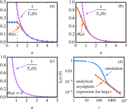
Figure 3: (a) The (red) solid line plots the analytical $\theta(a)$ vs. $a$ in Eq. (8), for the potential in Eq. (5b) in case (ii), with $\alpha=D=1$. The (blue) points represent the simulation results. The (magenta) dashed line plots the analytical expression (see SM ) of the inverse of the mean first-passage time. The vertical (gray) dashed line marks $a=a_{c}$. (b) Same plot as in (a) but for the case (i) in Eq. (5b) with $\mu=\alpha=D=1$ and $b=2$. (c) The (magenta) dashed line plots the inverse of the mean first-passage time for case (iii) in Eq. (5b), with $\alpha=D=\lambda=1$ and $b=c=e$. In this case $\theta(a)=0$ for all $a$. (d) The (blue) points represent simulation results for the survival probability $S_{a}(t|0)$ for the same potential as in (c), while the (red) dashed line represents the asymptotic decay of $S_{a}(t|0)$ in Eq. (13).

We now turn to the cases (i) and (iii) in Eq. (5b). While calculations in these two cases can also be carried out by mapping to the quantum problem (which indeed helps understanding the physics better), computationally it turns out to be more convenient to use a shorter backward Fokker-Planck approach Risken1984 ; SM2005 ; BMS2013 for the survival probability $S_{a}(t|x_{0})$ where the starting position $x_{0}$ is treated as a variable. The first-passage probability is then derived from the relation $F_{a}(t|x_{0})=-\partial_{t}S_{a}(t|x_{0})$. The backward Fokker-Planck equation reads

$$\frac{\partial S_{a}}{\partial t}=D\frac{\partial^{2}S_{a}}{\partial x_{0}^{2}}-U^{\prime}(x_{0})\,\frac{\partial S_{a}}{\partial x_{0}}$$ (9)

with the initial condition $S_{a}(0|x_{0})=1$ and the boundary conditions, $S_{a}(t|x_{0}\to-\infty)=1$ and $S_{a}(t|x_{0}=a)=0$. Skipping details (see SM ), the solution in the Laplace space $\tilde{S}_{a}(s|x_{0})=\int_{0}^{\infty}S_{a}(t|x_{0})\,e^{-st}\,dt$, reads

$$\tilde{S}_{a}(s|0)=\frac{1}{s}\bigl{[}1-\tilde{F}_{a}(s|0)\bigr{]}$$ (10)

where the Laplace transform of the first-passage time distribution is given by

$$\tilde{F}_{a}(s|0)=\frac{p}{B(s)}\,e^{-(\alpha+p)a/(2D)}\,\chi(s),$$ (11)

with $p=\sqrt{\alpha^{2}+4Ds}$ and the expressions of $B(s)$ and $\chi(s)$—which are different in the cases (i) and (iii)—are given in SM . Analyzing $\tilde{F}_{a}(s|0)$, we find that $s=-\alpha^{2}/(4D)$ is no longer a branch point.

In case (i), where $U(x)\sim x^{2}$ as $x\to-\infty$, the quantum potential $V(x)$ in Eq. (3) also diverges $\sim x^{2}$ as $x\to-\infty$. Hence, the quantum problem has only bound states with discrete spectrum. By analyzing (see SM ) Eq. (11), we indeed find that the denominator $B(s)$ has infinite number of zeros—equivalently, $\tilde{F}_{a}(s|0)$ has infinite number of poles—on the negative line $-\infty<s<0$. This infinite set of poles $-\infty<\dotsb<s_{2}^{*}(a)<s_{1}^{*}(a)<s_{0}^{*}(a)<0$ corresponds to having only bound states with discrete energy levels $E_{i}(a)=-s_{i}^{*}(a)$ with $i=0,1,\dotsc,\infty$. Therefore, both the first-passage and the survival probability decays as $F_{a}(t|0)\sim S_{a}(t|0)\sim e^{-\theta(a)t}$, where $\theta(a)=E_{0}(a)=-s_{0}^{*}(a)$. Figure 3 (b) plots $\theta(a)$ as a function of $a$ together with $1/T_{a}(0)$.

Turning now to case (iii), where $U(x)\sim c\,\ln(-x)$ as $x\to-\infty$ in Eq. (5b), we chose, for simplicity, $\lambda=1$ and $c>D$. The latter condition ensures that in the absence of the absorbing wall at $a$, the stationary Boltzmann distribution $P(x,t\to\infty)\propto e^{-U(x)/D}$ is normalizable, i.e., $\int e^{-U(x)/D}\,dx$ is finite. Diffusion in such potentials with logarithmic tails has been studied extensively in various contexts such as in the denaturation process of DNA molecules BKM2009 , momentum distribution of cold atoms in optical lattices CDC1991 ; MEZ1996 ; KB2010 , among many others EH2005 ; LMS2005 ; CDR2009 ; Bray2000 ; Lo2002 ; HMS2011 ; RR2020 . In this case, the associated quantum potential $V(x)\to 0$ as $x\to-\infty$ from Eq. (3). Therefore, the quantum problem has only scattering states and no bound state. Indeed we find that $\tilde{F}_{a}(s|0)$ does not have any pole, even when $a\to\infty$. Anticipating the scattering states to lead to a power-law decay for $F_{a}(t|0)$ at late times, we analyze $\tilde{F}_{a}(s|0)$ near $s=0$, and from it deduce the asymptotic decay of $F_{a}(t|0)$ for large $t$. For a noninteger $\nu=(1+c/D)/2\in(n,n+1)$ with $n\geq 1$ being an integer, we find the following late time decay SM

$$F_{a}(t|0)=\nu\,a_{\nu}\,t^{-(\nu+1)}+o(t^{-(\nu+1)}).$$ (12)

where the amplitude $a_{\nu}$ can be computed explicitly SM . Consequently, the survival probability decays as

$$S_{a}(t|0)=\int_{t}^{\infty}F_{a}(t^{\prime}|0)\,dt^{\prime}=a_{\nu}\,t^{-\nu}+o(t^{-\nu}).$$ (13)

For integer values of $\nu$, there are additional $\ln t$ corrections. Hence, $\theta(a)=-\lim_{t\to\infty}\,t^{-1}\,\ln S_{a}(t|0)$ is zero for all $a$, while $1/T_{a}(0)$ is still nonzero and a monotonic function of $a$ [see Fig. 3 (c)]. In Fig. 3 (d), we verify the analytical prediction in Eq. (13) by numerical simulation.

In conclusion, our main result is that $\theta(a)$, as a function of decreasing target location $a$, has substantially different behaviors depending on the far negative tail of the confining potential $U(x)$. Far negative tail actually means $|x|\gg\xi$ for negative $x$, where $\xi$ denotes the typical width of the confining potential near its minimum, e.g., in the context of animal foraging for food, $\xi$ denotes the size of the home range. At first sight, this may look puzzling: why does the far negative tail of $U(x)$ affect $\theta(a)$ for $a\sim O(1)>0$? Qualitatively, if the potential is sufficiently confining [$U(x)\sim|x|^{\gamma}$ as $-x\gg\xi$ with $\gamma>1$], the typical trajectory remains confined and the particle feels the presence of the absorbing barrier located at $a$ more strongly. However, for $\gamma\leq 1$ (where the spectrum of the associated quantum problem has scattering states), the typical trajectory wanders off to the far negative side (since the potential is not sufficiently confining on that side), and hence the particle becomes more insensitive to the presence of the absorbing barrier at $a>0$. In this Letter, this qualitative understanding is made precise via the exact analysis of the associated quantum problem. This led to a surprising “freezing” transition of $\theta(a)$ at a critical value $a_{c}$ for $\gamma=1$. We expect this freezing transition to be robust, e.g., it will hold for finite systems when the system size $L\gg\xi$. Finally, the potentials discussed in the Letter can be tailored by using holographic optical tweezers and confining the movements of colloidal particles to a quasi-one-dimensional line using a microfluidic device CGCKT20 , leading to a possible experimental measurement of $\theta(a)$.

S. N. M. acknowledges the support from the Science and Engineering Research Board (SERB, government of India), under the VAJRA faculty scheme (No. VJR/2017/000110) during a visit to Raman Research Institute, where part of this work was carried out.

References

- (1) P. Hänggi, P. Talkner, and M. Borkovec, Rev. Mod. Phys. 62, 251 (1990).
- (2) L. Farkas, Z. Phys. Chem. (Leipzig) 125, 236 (1927).
- (3) R. Kaischew and I. N. Stranski, Z. Phys. Chem. B 26, 317 (1934).
- (4) R. Becker and W. Döring, Ann. Phys. (Leipzig) 24, 719 (1935).
- (5) H. A. Kramers, Physica (Utrecht) 7, 284 (1940).
- (6) N. G. van Kampen, Stochastic Processes in Physics and Chemistry (North-Holland, Amsterdam, New York, 1981).
- (7) J. H. Van’t Hoff, in Etudes De Dynamiques Chimiques (F. Muller and Co., Amsterdam, 1884), p. 114; T. Ewan, Studies in Chemical Dynamics (London, 1896).
- (8) S. Arrhenius, Z. Phys. Chem. (Leipzig) 4, 226 (1889).
- (9) L. A. Pontryagin, A. Andronov, and A. Vitt, Zh. Eksp. Teor. Fiz. 3, 165 (1933); J. B. Barbour, in Noise in Nonlinear Dynamics, edited by F. Moss and P. V. E. McClintock, No. 1 (Cambridge University Press, Cambridge, 1989), p. 329.
- (10) H. Risken, The Fokker Planck Equation (Springer, Berlin, New York, 1984).
- (11) S. N. Majumdar, Curr. Sci. 77, 370 (1999).
- (12) S. Redner, A guide to first-passage processes (Cambridge University Press, Cambridge, 2001).
- (13) S.N. Majumdar, Curr. Sci. 89, 2076 (2005).
- (14) A. J. Bray, S.N. Majumdar, and G. Schehr, Adv. in Phys. 62, 225 (2013).
- (15) A. Godec and R. Metzler, Sci. Rep. 6, 20349 (2016).
- (16) D. Hartich and A. Godec, New J. Phys. 20, 112002 (2018).
- (17) D. Hartich and A. Godec, J. Stat. Mech. 024002 (2019).
- (18) D. Hartich and A. Godec, J. Phys. A: Math. Theor. 52, 244001 (2019).
- (19) R. J. Martin, M. J. Kearney, and R. V. Craster, J. Phys. A: Math. Theor. 52, 134001 (2019).
- (20) O. Bénichou, C. Loverdo, M. Moreau, and R. Voituriez, Rev. Mod. Phys. 83, 81 (2011).
- (21) G. M. Viswanathan, M. G. E. de Luz, E. P. Raposo, and H. E. Stanley, The physics of Foraging: An Introduction to Random Searches and Biological Encounters (Cambridge University Press, New York, 2011).
- (22) A. Godec and R. Metzler, Phys. Rev. X, 6, 041037 (2016).
- (23) See Supplemental Material for details.
- (24) A. Bar, Y. Kafri, and D. Mukamel, J. Phys. Condens. Matter 21, 034110 (2009).
- (25) Y. Castin, J. Dalibard, and C. Cohen-Tannoudji, in Light Induced Kinetic Effects on Atoms, Ions and Molecules, edited by L. Moi et al. (ETS Editrice, Pisa, Italy, 1991).
- (26) S. Marksteiner, K. Ellinger, and P. Zoller, Phys. Rev. A 53, 3409 (1996).
- (27) D. A. Kessler and E. Barkai, Phys. Rev. Lett. 105, 120602 (2010).
- (28) M. R. Evans and T. Hanney, J. Phys. A 38, R195 (2005).
- (29) E. Levine, D. Mukamel, and G. M. Schutz, Europhys. Lett. 70, 565 (2005).
- (30) A. Campa, T. Dauxois, and S. Ruffo, Phys. Rep. 480, 57 (2009).
- (31) A. J. Bray, Phys. Rev. E 62, 103 (2000).
- (32) C.-C. Lo, L. A. Nunes Amaral, S. Havlin, P. C. Ivanov, T. Penzel, J.-H. Peter, and H. E. Stanley, Europhys. Lett. 57, 625 (2002).
- (33) O. Hirschberg, D. Mukamel, and G. M. Schutz, Phys. Rev. E 84, 041111 (2011).
- (34) S. Ray and S. Reuveni, J. Chem. Phys. 152, 234110 (2020).
- (35) M. Chupeau, J. Gladrow, A. Chepelianskii, U. F. Keyser, and E. Trizac, Proc. Acad. Natl. Sci. U.S.A. 117, 1383 (2020).