Black hole genealogy: Identifying hierarchical mergers with gravitational waves

Abstract

In dense stellar environments, the merger products of binary black hole mergers may undergo additional mergers. These hierarchical mergers are naturally expected to have higher masses than the first generation of black holes made from stars. The components of hierarchical mergers are expected to have significant characteristic spins, imprinted by the orbital angular momentum of the previous mergers. However, since the population properties of first-generation black holes are uncertain, it is difficult to know if any given merger is first-generation or hierarchical. We use observations of gravitational waves to reconstruct the binary black hole mass and spin spectrum of a population including the possibility of hierarchical mergers. We employ a phenomenological model that captures the properties of merging binary black holes from simulations of globular clusters. Inspired by recent work on the formation of low-spin black holes, we include a zero-spin subpopulation. We analyze binary black holes from LIGO and Virgo’s first two observing runs, and find that this catalog is consistent with having no hierarchical mergers. We find that the most massive system in this catalog, GW170729, is mostly likely a first-generation merger, having a $4\%$ probability of being a hierarchical merger assuming a $5\times 10^{5}M_{\odot}$ globular cluster mass. Using our model, we find that $99\%$ of first-generation black holes in coalescing binaries have masses below $44$ $M_{\odot}$, and the fraction of binaries with near-zero component spins is less than $0.16$ ($90\%$ probability). Upcoming observations will determine if hierarchical mergers are a common source of gravitational waves.

1 Introduction

The gravitational-wave (GW) observations of LIGO (Aasi et al., 2015) and Virgo (Acernese et al., 2015) have revealed a population of stellar-mass binary black holes (Abbott et al., 2016a, 2019a, 2020b). These black holes range in mass over $\sim 7$–$50M_{\odot}$, extending beyond the masses observed in X-ray binaries (Abbott et al., 2016b; Miller & Miller, 2014). Since black hole systems can encode information about how their progenitor systems evolve (Abbott et al., 2016b, 2017a; Mandel & Farmer, 2018), this new population of black holes observed via GWs has broadened our understanding of the physical processes that shape the mass spectrum of stellar-origin black holes. Already, GW observations hint at a dearth of stellar-mass black holes with component masses $\gtrsim 45M_{\odot}$ (Abbott et al., 2019b), as predicted by theory decades ago.

Black holes are the end point of stellar evolution for stars $\gtrsim 20M_{\odot}$ (Woosley et al., 2002). Though more massive stars typically result in more massive black holes, the mapping between initial stellar mass and remnant mass is affected by many physical processes including stellar winds, stellar rotation, and binary interactions (Belczynski et al., 2010; Spera et al., 2015; Kruckow et al., 2018; Neijssel et al., 2019; Ertl et al., 2020). Additionally, stellar evolution does not predict a simple continuum that persists to arbitrarily high black hole masses. When stellar cores reach $\sim 50M_{\odot}$ they become become susceptible to pair instability (Fowler & Hoyle, 1964). In this process, high-energy photons undergo electron–positron pair production, causing a drop in the radiation pressure supporting the stellar core. The core subsequently contracts, increasing the temperature, triggering nuclear burning of carbon, oxygen, and silicon (Woosley & Heger, 2015). Stellar cores of $\sim 35$–$65M_{\odot}$ undergo pulsational pair instabilities (PPSNe; Woosley et al., 2007; Woosley, 2017; Marchant et al., 2019), where the star sheds large amounts of mass prior to collapse, limiting the resultant mass of the remnant black hole. Stars with cores of $\sim 65$–$135M_{\odot}$ are subject to pair-instability supernovae (PISNe; Barkat et al., 1967; Fryer et al., 2001; Heger & Woosley, 2002), where the instability results in the complete disruption of the star and no remnant black hole. Stellar evolution theory predicts a gap in the black hole mass spectrum between $\approx 45$–$135M_{\odot}$ (Belczynski et al., 2016; Spera & Mapelli, 2017; Stevenson et al., 2019).

Measuring the bounds of the PISN mass gap will provide insights into stellar evolution and fundamental physics (Farr et al., 2019; Farmer et al., 2019; van Son et al., 2020; Talbot & Thrane, 2018). However, one needs to account for the dynamical processes that can lead to black holes in this mass range. In dense stellar environments, such as globular clusters and nuclear star clusters, gravitational encounters of black holes in the cluster core harden the orbits of binary black hole systems, facilitating mergers within the cluster (e.g., Heggie, 1975; Banerjee et al., 2010; Rodriguez et al., 2016a).

If these merger products remain in the cluster environment, they can potentially merge again. These hierarchical mergers are characterized by a higher masses and spins than is typical of black holes born from stars (Miller & Hamilton, 2002; Gerosa & Berti, 2017; Fishbach et al., 2017; Kimball et al., 2020; Arca Sedda et al., 2020; Baibhav et al., 2020). Dense stellar environments are prime locations for facilitating such hierarchical mergers, which exhibit unique intrinsic properties that can be measured with GWs.

Identifying black holes formed through previous mergers requires knowledge of the initial mass spectrum of black holes formed through direct stellar collapse (Kimball et al., 2020; Doctor et al., 2019). Given the uncertainties in massive star evolution and binary stellar evolution, the properties of the natal black hole population are uncertain—it is something we aim to determine from GW observations. Therefore, it is essential to simultaneously infer the properties of the natal black hole population as part of our hierarchical mergers model. By doing so we can reconstruct valuable information about the origins of binary black holes. For example, the mass spectrum of the natal black hole population contains information on the stellar mass-loss rates (Stevenson et al., 2015; Barrett et al., 2018). Meanwhile, the fraction of merger products that go on to merge again encodes information on the physics of dense stellar environments. Only a fraction of black holes formed from binary black hole mergers are retained within a cluster, since the merger product receives a recoil kick from the anisotropic GW emission (Blanchet, 2014; Campanelli et al., 2007; Lousto & Zlochower, 2011; Sperhake, 2015) or can be subsequently ejected through close dynamical interactions with other objects (Heggie, 1975; Portegies Zwart & McMillan, 2000; Moody & Sigurdsson, 2009; Downing et al., 2011). The fraction retained depends on the mass and size of the cluster, and crucially upon the spins of the progenitor black holes (Rodriguez et al., 2018, 2019; Gerosa & Berti, 2019; Banerjee, 2020). Furthermore, the number of hierarchical mergers may enable us to determine the dominant formation channel for binary black holes.

In this study, we investigate how hierarchical binary black hole mergers can be identified within a population of GW observations. We focus on formation in globular clusters, where, due to the shallow gravitational potential, merger products typically cannot proceed through more than one additional merger before being ejected. We refer to the population of black holes formed from standard stellar evolution as first generation (1G), and black holes that result from a binary black hole merger of 1G components as second generation (2G). Hierarchical mergers, involving one or more 1G black hole, are denoted 1G+2G and 2G+2G depending on whether the merger contains one or two 2G black holes. First-generation mergers are denoted 1G+1G.

Using simple phenomenological models for the properties of 1G+1G, 1G+2G, and 2G+2G binaries, we perform hierarchical inference to determine the properties and rates of these different subpopulations. These phenomenological models are a natural extension of previous studies of the mass and spin distributions of binary black holes (Fishbach & Holz, 2017; Talbot & Thrane, 2018; Wysocki et al., 2019; Abbott et al., 2019b) and are explained in Sec. 2. The hierarchical inference methodology using these models is explained in Sec. 3. We apply our methodology to the set of binary black holes presented in GWTC-1 (Abbott et al., 2019a) in Sec. 4, and discuss the inferred population hyperparameters in Appendix A. In Appendix B, we consider how results change upon adding GW190412 (Abbott et al., 2020b) to the GWTC-1 population. In future work, we will extend this analysis to events found by external searches (Nitz et al., 2020; Venumadhav et al., 2019; Zackay et al., 2019b; Venumadhav et al., 2020; Zackay et al., 2019a). We find that observations are consistent with all binaries being 1G+1G (Kimball et al., 2020; Chatziioannou et al., 2019; Yang et al., 2019); however, if we include the possibility that some 1G black holes are born with near-zero spins (Qin et al., 2018; Fuller & Ma, 2019; Belczynski et al., 2020), we find a small probability of GW170729 containing a 2G black hole using our models for globular clusters. Our conclusions are summarized in Sec. 5.

2 Population model

Phenomenological models are computationally efficient tools for parameterizing black hole population properties. The model we develop in this study approximates the detectable population of merging binary black holes from globular clusters, and is designed to capture the main features of binaries formed through hierarchical mergers. The model is constructed using population hyperparameters $\boldsymbol{\Lambda}$ that describe the 1G+1G black hole population.

We assume that the overall population of binary black holes consists of three subpopulations: 1G+1G, 1G+2G and 2G+2G binaries. We neglect the probability of higher-order mergers (containing a $\geq$ 2G component) in this analysis since the number of these mergers is negligible in globular cluster models (Rodriguez et al., 2019; Arca Sedda et al., 2020). However, dense stellar environments such as those in galactic nuclei, nuclear star clusters (Antonini et al., 2019), and active galactic nucleus disks (Yang et al., 2019), may retain higher-order merger products and our approach can be expanded to include their contribution.

The fractions of total mergers associated with each generation are denoted $\zeta_{\textsf{1G+1G}}{}(\boldsymbol{\Lambda})$, $\zeta_{\textsf{1G+2G}}{}(\boldsymbol{\Lambda})$ and $\zeta_{\textsf{2G+2G}}{}(\boldsymbol{\Lambda})$. Since only a small fraction of 2G black holes are retained in the fiducial cluster and able to form a new binary, we expect that $\zeta_{\textsf{1G+1G}}{}(\boldsymbol{\Lambda})\gg\zeta_{\textsf{1G+2G}}{}(\boldsymbol{\Lambda})\gg\zeta_{\textsf{2G+2G}}{}(\boldsymbol{\Lambda})$. By unitarity, we have

$$\zeta_{\textsf{1G+1G}}{}(\boldsymbol{\Lambda})+\zeta_{\textsf{1G+2G}}{}(\boldsymbol{\Lambda})+\zeta_{\textsf{2G+2G}}{}(\boldsymbol{\Lambda})=1.$$ (1)

The fraction of binaries in each subpopulation depends upon the population properties of the 1G+1G binary black holes. In particular, the distributions of component spins and mass ratio have a strong effect on the recoil kick during merger.

For each generation, we define an astrophysically motivated prior on the properties $\boldsymbol{\theta}$ describing individual binary black holes, such as their masses and spins. We decompose the overall prior for a given generation into priors on the primary mass $m_{1}$, mass ratio $q=m_{2}/m_{1}$, spin magnitudes $\chi_{1}$ and $\chi_{2}$, spin orientations ${z_{1}}\equiv\cos\theta_{1}$ and ${z_{2}}\equiv\cos\theta_{2}$ (where $\theta_{i}$ is the angle between the black hole spin and the orbital angular momentum vector), and extrinsic parameters ${\vartheta}$. The prior on the extrinsic parameters is assumed to be the same for all generations: mergers are uniformly distributed in comoving volume and we employ standard priors for other extrinsic parameters.

The population model is described in the following subsections. In Sec. 2.1, we describe a model for the mass and spin distributions of 1G+1G binary black holes (Wysocki et al., 2019; Talbot & Thrane, 2018, 2017; Abbott et al., 2019b). The population of 1G+1G binary black holes forms the cornerstone of our models, and the properties of merger products are set based upon this. In Sec. 2.2, we describe our prescription to estimate the mass and spin distributions of 1G+2G and 2G+2G binaries given the 1G+1G distribution. In Sec. 2.3, we describe our method for calculating the generational fractions $\zeta_{\textsf{1G+1G}}{}$, $\zeta_{\textsf{1G+2G}}{}$, and $\zeta_{\textsf{2G+2G}}{}$ given our population model. The hierarchical inference method we outline in Sec. 3 can be adapted to use alternative phenomenological models as improved descriptions are developed. The phenomenological method presented here predicts distributions that are qualitatively similar to simulations of globular clusters (e.g., Rodriguez et al., 2019).

2.1 1G+1G binaries

2.1.1 Primary mass

Following Abbott et al. (2019b), we model the distribution of 1G+1G black hole primary mass $m_{1}$ using the prescription from Talbot & Thrane (2018)

$$\pi(m_{1}| \alpha,m_{\mathrm{min}},m_{\mathrm{max}},\lambda_{m},\mu_{m},\sigma_{m},\textsf{1G+1G}{})=$$

$$\left[(1-\lambda_{m})\mathcal{A}m_{1}^{\alpha}\Theta(m_{\mathrm{max}}-m_{1})\right.+$$

$$\left.\lambda_{m}\mathcal{B}N(m_{1}|\mu_{m},\sigma_{m})\right],$$ (2)

where $\left\{\alpha,m_{\mathrm{min}},m_{\mathrm{max}},\lambda_{m},\mu_{m},\sigma_{m},\right\}\in\boldsymbol{\Lambda}$ are the population hyperparameters defining this distribution. This model includes two components. The first is a truncated power-law distribution with spectral index $\alpha$ and a maximum mass of $m_{\mathrm{max}}$ (enforced by the Heaviside step function $\Theta$). The second is a Gaussian component with mean $\mu_{m}$ and standard deviation $\sigma_{m}$. The parameter $\lambda_{m}$ is a mixing fraction, which determines the fraction of binaries associated with either component. The factors $\mathcal{A}$ and $\mathcal{B}$ are normalization constants that depend on the other population hyperparameters. This mass distribution is chosen to enforce the expected cutoff in the black hole mass spectrum from PISNe (Heger et al., 2003; Belczynski et al., 2016; Fishbach & Holz, 2017), with the Gaussian capturing a buildup from PPSNe (Woosley, 2017; Marchant et al., 2019; Talbot & Thrane, 2018).

2.1.2 Mass ratio

Following Abbott et al. (2019b), we model the 1G+1G mass ratio $q$ using a power-law distribution (Talbot & Thrane, 2018),

$$\pi(q| m_{1},\beta_{q},m_{\mathrm{min}},\textsf{1G+1G}{})=\mathcal{C}(m_{1})m_{2}^{\beta_{q}}\Theta(m_{1}-m_{2}),$$ (3)

defined using population hyperparameters $\{m_{1},\beta_{q},m_{\mathrm{min}}\}\in\boldsymbol{\Lambda}$. Here $\beta_{q}$ is the power-law index, and $\mathcal{C}$ is a normalization constant.

2.1.3 Spin magnitudes

We assume that the spin magnitudes of both black holes $\chi_{1}$ and $\chi_{2}$ are described by the same distribution,

$$\pi(\chi|\lambda_{0},\alpha_{\chi},\beta_{\chi},\textsf{1G+1G}{})=\lambda_{0}\delta(\chi)+(1-\lambda_{0})\mathrm{B}(\chi|\alpha_{\chi},\beta_{\chi}),$$ (4)

described by population hyperparameters $\{\lambda_{0},\alpha_{\chi},\beta_{\chi}\}\in\boldsymbol{\Lambda}$ Here, $\mathrm{B}$ is a Beta distribution parameterized by shape parameters $\alpha_{\chi}$ and $\beta_{\chi}$ (Wysocki et al., 2019).

However, a simple Beta distribution will struggle to capture the morphology of the true population if a significant fraction of binary black holes have low ($\lesssim 0.01$) natal spins, which is anticipated to be the case if angular momentum transport in massive stars is efficient (Qin et al., 2018; Fuller & Ma, 2019). The mixing parameter $\lambda_{0}$ controls the fraction of black holes merging with negligible spin. We assume that the spin of the primary black hole in a binary is independent from the spin of the secondary black hole.

2.1.4 Spin orientation

The orientation of black hole spin can be parameterized using the cosine of the polar angle between the spin vector and the Newtonian orbital angular momentum $z_{i}=\cos\theta_{i}$. In Abbott et al. (2019b), the orientation of black hole spin was modeled using a mixture model (Talbot & Thrane, 2017)

$$\pi(z_{1},z_{2}| \zeta_{\mathrm{iso}},\sigma_{1},\sigma_{2},\textsf{1G+1G}{})=\zeta_{\mathrm{iso}}U(z_{1})U(z_{2})$$

$$+(1-\zeta_{\mathrm{iso}})N_{\mathrm{t}}(z_{1}|0,\sigma_{1})N_{\mathrm{t}}(z_{2}|0,\sigma_{2}),$$ (5)

defined with population hyperparameters $\{\zeta_{\mathrm{iso}},\sigma_{1},\sigma_{2}\}\in\boldsymbol{\Lambda}$. Here $\zeta_{\mathrm{iso}}$ is the fraction of binaries that are drawn from a distribution with isotropic spin orientations (uniform in $z_{1}$ and $z_{2}$). The isotropic distribution is expected for dynamically assembled binaries because the stellar progenitors did not coevolve. Binaries that are not drawn from this uniform distribution $U$ are drawn from a truncated normal distribution $N_{\mathrm{t}}$. The normal distribution is centered on $z=0$ corresponding to aligned spin with width determined by the standard deviations $\sigma_{1}$ and $\sigma_{2}$. The truncated normal distribution represents the binaries formed in the galactic field, where spins are predicted to be generally aligned, with some scatter due to supernova kicks (Rodriguez et al., 2016b). For this analysis, we set $\zeta_{\mathrm{iso}}=1$, which effectively adopts the framework that all binaries are dynamical mergers:

$$\pi(z_{1},z_{2}|\sigma_{1},\sigma_{2},\textsf{1G+1G}{})=U(z_{1})U(z_{2}).$$ (6)

For future work, this model could be extended to reintroduce $\zeta_{\mathrm{iso}}$ and only to consider hierarchical mergers from the fraction of events formed dynamically.

2.2 1G+2G and 2G+2G binaries

2.2.1 Primary mass

Our model for the primary mass distributions for 1G+2G and 2G+2G mergers is built on the premise that 2G+2G black holes are roughly twice as massive as 1G+1G black holes. We make the simplifying assumption that in a 1G+2G binary, the primary is always the 2G black hole (Kimball et al., 2020). Thus, the 1G+2G and 2G+2G primary mass spectra are modeled as

$$\pi(m_{1}|\boldsymbol{\Lambda},\textsf{1G+2G}{})\propto {}\>\pi\left(\frac{m_{1}}{2}\middle|\boldsymbol{\Lambda},\textsf{1G+1G}{}\right),$$ (7)

$$\pi(m_{1}|\boldsymbol{\Lambda},\textsf{2G+2G}{})\propto {}\>\pi\left(\frac{m_{1}}{2}\middle|\boldsymbol{\Lambda},\textsf{1G+1G}{}\right),$$ (8)

This representation is found to qualitatively match the results of globular cluster simulations (e.g., Rodriguez et al., 2018, 2019).

2.2.2 Mass ratio

Since we expect that 1G+2G and 2G+2G binaries are formed dynamically, the mass ratio distributions should depend upon mass segregation and the dynamical interactions that form binaries inside dense stellar environments. We calibrate our mass ratio distributions against the results of globular cluster simulations from Rodriguez et al. (2019). For 1G+2G binaries, we adopt a model where the mass ratio distribution peaks around $q\sim 0.5$. We find that the distribution recovered from cluster simulations may be approximated as

$$\pi(q|\boldsymbol{\Lambda},\textsf{1G+2G}{})\propto \begin{cases}\pi(q|\boldsymbol{\Lambda},\textsf{1G+1G}{})^{1.5}&q\leq 1/2\\ \pi(1-q|\boldsymbol{\Lambda},\textsf{1G+1G}{})^{-1.5}&q>1/2\end{cases}.$$ (9)

An alternative parameterization, producing a similar form, is given in Chatziioannou et al. (2019). The most important feature of the 1G+2G distribution is that it peaks away from $q=1$, as this distinguishes it from the 1G+1G and 2G+2G distributions.

For 2G+2G binaries we find that

$$\pi(q|\boldsymbol{\Lambda},\textsf{2G+2G}{})\propto {}\pi(q|\boldsymbol{\Lambda},\textsf{1G+1G}{})^{4}$$ (10)

produces qualitative agreement with predictions from Rodriguez et al. (2019). This distribution is more tightly peaked at $q\sim 1$ than the 1G+1G population, reflecting the preference for dynamically formed binary mergers to by dominated by the most massive components in the cluster (Heggie et al., 1996; Sigurdsson & Phinney, 1993; Downing et al., 2011).

2.2.3 Spins

The spin magnitude of post-merger remnants is primarily determined by the orbital angular momentum of the progenitor binary (Pretorius, 2005; Buonanno et al., 2008; Gonzalez et al., 2007). For typical binaries (with mass ratio $q\approx 1$ and low spins) the remnant spin is $\approx 0.67$. We therefore adopt for 1G+2G spins

$$\pi(\chi_{1}|\boldsymbol{\Lambda},\textsf{1G+2G}{})= {}\>\mathrm{B}(\chi_{1}|14.14,6.97),$$ (11)

$$\pi(\chi_{2}|\textsf{1G+2G}{})= {}\>\pi(\chi_{2}|\boldsymbol{\Lambda},\textsf{1G+1G}{}),$$ (12)

and for 2G+2G spins

$$\pi(\chi_{1}|\boldsymbol{\Lambda},\textsf{2G+2G}{})= {}\>\mathrm{B}(\chi_{1}|14.14,6.97),$$ (13)

$$\pi(\chi_{2}|\boldsymbol{\Lambda},\textsf{2G+2G}{})= {}\>\mathrm{B}(\chi_{2}|14.14,6.97).$$ (14)

Here, $\mathrm{B}(\mu,\sigma)$ is a beta function with shape parameters $\alpha_{\chi}$, $\beta_{\chi}$, which corresponds to a mean $0.67$ and standard deviation $0.1$ (Fishbach et al., 2017; Chatziioannou et al., 2019; Arca Sedda et al., 2020). We assume that the 1G+2G and 2G+2G spins are isotropically oriented, the same as for 1G+1G binaries.

2.3 Retention fraction

Given a 1G+1G population, the branching ratios of the 1G+2G and 2G+2G populations are determined by the fraction of 1G+1G merger products that are retained in the cluster. During the coalescence of a binary black hole, the anisotropic emission of GWs imparts a kick on the remnant. The magnitude of the kicks depends sensitively on the spin and mass ratio of the binary (Gonzalez et al., 2007; Campanelli et al., 2007; Bruegmann et al., 2008; Lousto & Zlochower, 2011; Varma et al., 2019), and can far exceed the typical escape velocities of globular clusters ($\sim 30$–$50~{}\mathrm{km\,s}^{-1}$ at $z=0$), ejecting merger products and leaving them unavailable to form new generations of binary black holes (Merritt et al., 2004; Moody & Sigurdsson, 2009; Varma et al., 2020). Therefore, the branching ratios of the 1G+2G and 2G+2G popoulations are sensitive to the distribution of mass ratios and component spins in the 1G+1G population, as well as the mass and size of the cluster.

In order to estimate the retention fraction, we begin by calculating the probability $P_{\mathrm{ret}}(\chi_{1},\chi_{2},q)$ that the remnant of a merging binary with component spins and mass ratio $(\chi_{1},\chi_{2},q)$ will be retained in a cluster potential following the GW recoil kick. For our cluster model, we adopt a Plummer potential (Plummer, 1911) with mass distribution

$$\rho_{p}(r)=\frac{3M_{\mathrm{c}}}{4\pi r_{\mathrm{c}}^{3}}\left(1+\frac{r^{2}}{a_{\mathrm{c}}^{2}}\right)^{-5/2}.$$ (15)

We assume a cluster mass $M_{\mathrm{c}}=5\times 10^{5}M_{\odot}$ and a Plummer radius $r_{\mathrm{c}}=1~{}\mathrm{pc}$ to represent a fiducial globular cluster. For a given $\{\chi_{1},\chi_{2},q\}$ we sample merger locations following Eq. (15) and sample component spin-tilts isotropically, then calculate recoil velocities according to Gerosa & Kesden (2016) and check against the local escape velocity to obtain $P_{\mathrm{ret}}(\chi_{1},\chi_{2},q)$.

Figure 1 shows $P_{\mathrm{ret}}(\chi_{1},\chi_{2},q)$ for the case of equal spin magnitudes. $P_{\mathrm{ret}}$ is negligible when component spins are $\gtrsim 0.1$, except in the regime of extreme mass ratios ($q\to 0$) where recoil velocities disappear. Therefore, nearly all 1G+1G binaries with appreciable spins will form merger products that are promptly ejected from the fiducial cluster and will be unable to form hierarchical mergers. We see that a subpopulation of 1G black holes with negligible spin, represented by the delta function in Eq. (4), is a key ingredient for hierarchical mergers.

For a population determined by population hyperparameters $\boldsymbol{\Lambda}$, we calculate the fraction $F_{\mathrm{ret}}$ of 1G+1G remnants that are retained in our fiducial cluster as

$$F_{\mathrm{ret}}(\boldsymbol{\Lambda})= \int\mathrm{d}q\int\mathrm{d}\chi_{1}\int\mathrm{d}\chi_{2}\,\pi(\chi_{1}|\boldsymbol{\Lambda},\textsf{1G+1G}{})$$ (16)

$$\pi(\chi_{2}|\boldsymbol{\Lambda},\textsf{1G+1G}{})\pi(q|\boldsymbol{\Lambda},\textsf{1G+1G}{})P_{\mathrm{ret}}(\chi_{1},\chi_{2},q).$$

Here, $\pi(q|\boldsymbol{\Lambda},\textsf{1G+1G}{})$ and $\pi(\chi|\boldsymbol{\Lambda},\textsf{1G+1G}{})$ are the 1G+1G mass ratio and component-spin distributions.

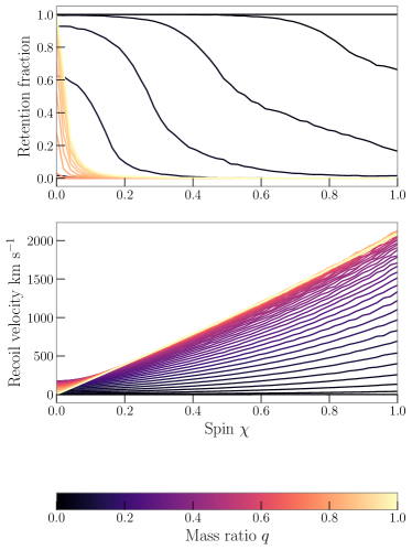
Figure 1: Top: the retention fractions $P_{\mathrm{ret}}$ assuming a $5\times 10^{5}M_{\odot}$ cluster with a $1~{}\mathrm{pc}$ Plummer radius. Bottom: recoil velocities for equal component-spin binary black holes, colored according to mass ratio $q\equiv m_{2}/m_{1}$. For each $\{\chi,q\}$ configuration, we sample spin orientations isotropically and plot the mean recoil velocity.

2.4 Branching ratios

Using $F_{\mathrm{ret}}$($\boldsymbol{\Lambda}$), we calculate hierarchical branching ratios given a 1G+1G population with mass and spin distributions determined by population hyperparameters $\boldsymbol{\Lambda}$. Let $R_{\textsf{1G+1G}{}}$, $R_{\textsf{1G+2G}{}}$, and $R_{\textsf{2G+2G}{}}$ be the rates of 1G+1G, 1G+2G, and 2G+2G mergers, respectively, averaged over the lifetime of the cluster. The number of 2G black holes available to form new binaries is proportional to $F_{\mathrm{ret}}R_{\textsf{1G+1G}}{}$. Therefore, we expect

$$R_{\textsf{1G+2G}}{}= \>\xi_{\textsf{1G+2G}}{}{}F_{\mathrm{ret}}(\boldsymbol{\Lambda})R_{\textsf{1G+1G}}{},$$ (17)

$$R_{\textsf{2G+2G}}{}= \>\xi_{\textsf{2G+2G}}{}{}[F_{\mathrm{ret}}(\boldsymbol{\Lambda})]^{2}R_{\textsf{1G+1G}}{},$$ (18)

where the constants of proportionality $\xi_{\textsf{1G+2G}}{}{}$ and $\xi_{\textsf{1G+2G}}{}{}$ are set by the dynamical processes within the cluster, such as the frequency at which binaries form. Based on comparison with simulations (Rodriguez et al., 2019), we find that $\xi_{\textsf{1G+2G}}{}{}\simeq 1/2$ and $\xi_{\textsf{2G+2G}}{}{}\simeq 1/8$ are good approximations. From the rates we can define branching ratios,

$$\Gamma_{\textsf{1G+2G}}{}\equiv \>\frac{R_{\textsf{1G+2G}}{}}{R_{\textsf{1G+1G}}{}}\propto F_{\mathrm{ret}}(\boldsymbol{\Lambda}),$$ (19)

$$\Gamma_{\textsf{2G+2G}}{}\equiv \>\frac{R_{\textsf{2G+2G}}{}}{R_{\textsf{1G+1G}}{}}\propto[F_{\mathrm{ret}}(\boldsymbol{\Lambda})]^{2}$$ (20)

Since $F_{\mathrm{ret}}$ is small, we have $\Gamma_{\textsf{2G+2G}}{}\ll\Gamma_{\textsf{1G+2G}}{}\ll 1$.

We combine these branching ratios with our individual 1G+1G, 1G+2G, and 2G+2G population distributions to construct a multigenerational mixture model:

$$\pi_{\mathrm{hier}}({\mathrm{\theta}}|\boldsymbol{\Lambda})=\, \>\zeta_{\textsf{1G+1G}{}}(\boldsymbol{\Lambda})\pi(\boldsymbol{\theta}|\boldsymbol{\Lambda},\textsf{1G+1G}{})$$

$$+\zeta_{\textsf{1G+2G}{}}(\boldsymbol{\Lambda})\pi(\boldsymbol{\theta}|\boldsymbol{\Lambda},\textsf{1G+2G}{})$$

$$+\zeta_{\textsf{2G+2G}{}}(\boldsymbol{\Lambda})\pi(\boldsymbol{\theta}|\boldsymbol{\Lambda},\textsf{2G+2G}{}),$$ (21)

where

$$\zeta_{\textsf{1G+1G}{}}= \>\frac{1}{1+\Gamma_{\textsf{1G+2G}{}}+\Gamma_{\textsf{2G+2G}{}}},$$ (22)

$$\zeta_{\textsf{1G+2G}{}}= \>\frac{\Gamma_{\textsf{1G+2G}{}}}{1+\Gamma_{\textsf{1G+2G}{}}+\Gamma_{\textsf{2G+2G}{}}},$$ (23)

$$\zeta_{\textsf{2G+2G}{}}= \>\frac{\Gamma_{\textsf{2G+2G}{}}}{1+\Gamma_{\textsf{1G+2G}{}}+\Gamma_{\textsf{2G+2G}{}}}.$$ (24)

We use the GWTC-1 catalog of GW observations to constrain this model, and infer the population hyperparameters $\boldsymbol{\Lambda}$, and obtain the odds that any of the observations are from a hierarchical merger.

3 Population Inference

Given a set of population hyperparameters $\boldsymbol{\Lambda}$, the overall likelihood of an observation is

$$\mathcal{L}_{\mathrm{hier}}(d_{i}|\boldsymbol{\Lambda})=\frac{1}{P_{\mathrm{det}}(\boldsymbol{\Lambda})}\int\mathrm{d}\boldsymbol{\theta}\,L(d_{i}|\boldsymbol{\theta})\pi_{\mathrm{hier}}(\boldsymbol{\theta}|\boldsymbol{\Lambda}),$$ (25)

where we use $d_{i}$ to denote the GW data associated with the $i$-th observation, $L(d_{i}|\boldsymbol{\theta})$ is the likelihood of the data given the source parameters $\boldsymbol{\theta}$ (Cutler & Flanagan, 1994; Abbott et al., 2016c), $\pi_{\mathrm{hier}}(\boldsymbol{\theta}|\boldsymbol{\Lambda})$ is the population model defined in Sec. 2, and $P_{\mathrm{det}}(\boldsymbol{\Lambda})$ is the fraction of all astrophysical events which are observed and accounts for selection biases (Thrane & Talbot, 2019; Mandel et al., 2019). The fraction $P_{\mathrm{det}}(\boldsymbol{\Lambda})$ scales as the surveyed space-time volume $VT(\boldsymbol{\Lambda})$ of the detector network for a binary black hole population with population hyperparameters $\boldsymbol{\Lambda}$; we calculate $VT(\boldsymbol{\Lambda})$ analytically following Finn & Chernoff (1993), using a single-detector network with a median (over observing times from the first and second observing runs) LIGO Hanford noise curve and signal-to-noise ratio threshold of $8$. The overall likelihood in Eq. (25) can be broken into pieces associated with each generation,

$$\mathcal{L}_{\mathrm{hier}}(d_{i}|\boldsymbol{\Lambda})= {}\>\frac{1}{P_{\mathrm{det}}(\boldsymbol{\Lambda})}\left[\zeta_{\textsf{1G+1G}}{}(\boldsymbol{\Lambda})\mathcal{L}(d_{i}|\boldsymbol{\Lambda},\textsf{1G+1G}{})\right.$$

$$+\left.{}\zeta_{\textsf{1G+2G}}{}(\boldsymbol{\Lambda})\mathcal{L}(d_{i}|\boldsymbol{\Lambda},\textsf{1G+2G}{})\right.$$

$$+\left.{}\zeta_{\textsf{2G+2G}}{}(\boldsymbol{\Lambda})\mathcal{L}(d_{i}|\boldsymbol{\Lambda},\textsf{2G+2G}{})\right],$$ (26)

where

$$\mathcal{L}(d_{i}|\boldsymbol{\Lambda},\textsf{1G+1G}{})=\int\mathrm{d}\boldsymbol{\theta}\,L(d_{i}|\boldsymbol{\theta})\pi(\boldsymbol{\theta}|\boldsymbol{\Lambda},\textsf{1G+1G}{}),$$ (27)

and likelihoods for the other generations are defined similarly.

For a set of $N$ detections (described by data $\vec{d}$), the total likelihood becomes

$$\mathcal{L}_{\mathrm{tot}}(\vec{d}|\boldsymbol{\Lambda})= \prod_{i}^{N}\mathcal{L}_{\mathrm{hier}}(d_{i}|\boldsymbol{\Lambda}).$$ (28)

To calculate the total likelihood, we use samples drawn from the black hole parameter posterior probability distributions

$$p(\boldsymbol{\theta}|d_{i})=\frac{L(d_{i}|\boldsymbol{\theta},\theta)\pi(\boldsymbol{\theta}|\varnothing)}{Z_{\varnothing}(d_{i})},$$ (29)

calculated for each event using some fiducial parameter prior distribution $\pi(\boldsymbol{\theta}|\varnothing)$ which does not depend on the population hyperparameters. Taking $n_{i}$ parameter posterior samples for the $i$-th event,

$$\mathcal{L}_{\mathrm{tot}}(\vec{d}|\boldsymbol{\Lambda})\simeq \prod_{i}^{N}\frac{1}{P_{\mathrm{det}}(\boldsymbol{\Lambda})}\frac{Z_{\varnothing}(d_{i})}{n_{i}}\sum_{k}^{n_{i}}\frac{\pi(\boldsymbol{\theta}^{k}|\boldsymbol{\Lambda})}{\pi(\boldsymbol{\theta}^{k}|\varnothing)},$$ (30)

where $\boldsymbol{\theta}^{k}$ indicates the parameters of the $k$-th sample (Thrane & Talbot, 2019; Mandel et al., 2019).

In the case where our 1G+1G spin distribution includes the delta function at $0$, we alter this approach to account for the lack of parameter estimation samples with precisely zero component spin. For each event, we produce posterior samples with two fiducial priors (which are identical except for the component spins): one uniform in spin magnitude $\pi_{\chi}(\boldsymbol{\theta}|\varnothing)$, which enables us to sample the entire range of spins, and one where the spin is always zero $\pi_{0}(\boldsymbol{\theta}|\varnothing)$, which is applicable to the delta function model.

In this case, the 1G+1G term in Eq. (30) becomes

$$\mathcal{L}(d_{i}|\boldsymbol{\Lambda},\textsf{1G+1G}{}{})\simeq {}\>\frac{1}{n_{i}}\left[\lambda_{0}\sum_{j}^{n_{i,0}}\frac{\pi(\boldsymbol{\theta}^{j}|\boldsymbol{\Lambda},\textsf{1G+1G}{})}{\pi_{0}(\boldsymbol{\theta}^{j}|\varnothing)}\right.$$

$${}\left.+(1-\lambda_{0})\sum_{k}^{n_{i,\chi}}\frac{\pi(\boldsymbol{\theta}^{j}|\boldsymbol{\Lambda},\textsf{1G+1G}{})}{\pi_{\chi}(\boldsymbol{\theta}^{k}|\varnothing)}\right].$$ (31)

Here, $n_{i,0}$ and $n_{i,\chi}$ are the number of samples included using the zero-spin and uniform-spin respectively, and $n_{i}=n_{i,0}+n_{i,\chi}$ is the total number of samples used; the ratio of the number of zero- and uniform-spin samples is the ratio of the evidences calculated with the two priors,

$$\frac{n_{i,0}}{n_{i,\chi}}=\frac{Z_{0}(d_{i})}{Z_{\chi}(d_{i})}=\frac{\int\mathrm{d}\boldsymbol{\theta}L(d_{i}|\theta)\pi_{0}(\boldsymbol{\theta}|\varnothing)}{\int\mathrm{d}\boldsymbol{\theta}L(d_{i}|\boldsymbol{\theta})\pi_{\chi}(\boldsymbol{\theta}|\varnothing)}.$$ (32)

This procedure allows us to calculate the population likelihood even though the delta function and Beta distribution components of the spin model from Eq. (4) have different ranges of support.

We use hierarchical Bayesian inference to construct a posterior for our population hyperparameters

$$p(\boldsymbol{\Lambda}|\vec{d})=\frac{\mathcal{L}_{\mathrm{hier}}(\vec{d}|\boldsymbol{\Lambda})\pi(\boldsymbol{\Lambda})}{\int\mathrm{d}\boldsymbol{\Lambda}\mathcal{L}_{\mathrm{hier}}(\vec{d}|\boldsymbol{\Lambda})\pi(\boldsymbol{\Lambda})},$$ (33)

where $\pi(\boldsymbol{\Lambda})$ is our prior for the population hyperparameters. With the exception of $m_{\mathrm{max}}$, we take this prior to be flat (Abbott et al., 2019b). To account for uncertainties in the location of the PISN mass gap inherent in different sets of assumptions about nuclear reaction rates, stellar rotation, accretion, and fallback (Farmer et al., 2019; Mapelli et al., 2020; van Son et al., 2020), we take a Gaussian prior on $m_{\mathrm{max}}$ with a mean of $50M_{\odot}$ and standard deviation of $10M_{\odot}$.

We use gwpopulation (Talbot et al., 2019) and dynesty (Speagle, 2020) within the Bilby framework (Ashton et al., 2019) to sample the likelihoods in Eq. (28) and Eq. (3). Parameter estimation for each event is also performed using Bilby (Romero-Shaw et al., 2020), following the settings used to produce GWTC-1 results (Abbott et al., 2019a). GW data from LIGO and Virgo are obtained from the Gravitational Wave Open Science Center (Abbott et al., 2019c).

4 Application to GWTC-1

4.1 Inferred Populations

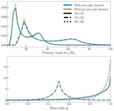
Figure 2: Posterior predictive distributions for primary mass $m_{1}$ and mass ratio $q$. The solid, dashed, and dotted lines are the 1G+1G, 1G+2G, 2G+2G distributions, respectively. The 1G+2G and 2G+2G primary masses are drawn from the same distributions. In blue, we plot the distributions inferred when allowing for the zero-spin formation channel, and the distributions inferred when excluding this channel are plotted in orange.

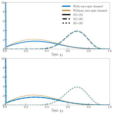
Figure 3: Posterior predictive distributions for the component black hole spins. The solid, dashed, and dotted lines are the 1G+1G, 1G+2G, 2G+2G distributions, respectively. The 1G+2G and 2G+2G primary spins are drawn from the same distributions, as are the 1G+1G and 1G+2G secondary spins. In blue, we plot the distributions inferred when allowing for the zero-spin formation channel, and distributions inferred when excluding this channel are plotted in orange.

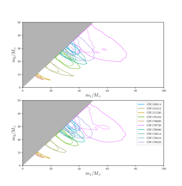
Figure 4: Reweighted GWTC-1 mass posteriors using our inferred hierarchical population model as a prior. Contours indicate the $90\%$ credible areas. The original posteriors from Abbott et al. (2019a) are indicated with solid lines, and the reweighted posteriors are shown with dashed lines. Top: results reweighted using the model inferred when excluding the zero-spin channel. Bottom: results reweighted using the population model inferred when allowing for the zero-spin formation channel. The exclusion of the zero-spin channel pushes the highest-mass events toward lower masses. Including zero-spin allows for more retained 2G black holes and hence more efficient hierarchical mergers, which, in turn, allows for larger masses. In both cases, the region of support at high primary mass ($\sim 60M_{\odot}$) in the reweighted GW170729 posterior is due to the hierarchical component of the population prior.

We apply the above analysis using the $10$ binary black hole observations contained in GWTC-1 (Abbott et al., 2019a), and infer population hyperparameters for our hierarchical model. The inferred population hyperparameters are discussed in detail in Appendix A. We plot the posterior predictive distributions for the 1G+1G, 1G+2G, and 2G+2G populations in Fig. 2 and Fig. 3. The population hyperparameters governing the 1G+1G mass distribution (see Fig. 2 in Appendix A) are consistent with the results in Abbott et al. (2019b). The Gaussian mass component corresponding to PPSN buildup is well constrained to $\mu_{m}\simeq 22$–$38$, but we recover our prior on the location of the PISN maximum-mass cutoff $m_{\mathrm{max}}$. We find that $99\%$ of 1G+1G black holes are less than $44M_{\odot}$, in agreement with $45M_{\odot}$ found in Abbott et al. (2019b), and that $99\%$ of black holes in the combined multigeneration population are less than $45M_{\odot}$. In Fig. 10 of Appendix A, we show population hyperparameters for the 1G+1G spin distribution.

The fraction $\lambda_{0}$ of black holes from the zero-spin formation channel is constrained to be less than $0.32$ at the $99\%$ credible level, and is consistent with $\lambda_{0}=0$. Therefore, these GW observations suggest that at least some 1G+1G binary black holes have spinning components, consistent with Miller et al. (2020), and not all 1G black holes have extremely low ($<0.01$) spins as would be expected if all progenitor stars had efficient angular momentum transfer (Fuller & Ma, 2019). We find that $90\%$ of 1G+1G primary black holes have a spin magnitude less than $0.57$.

In the bottom panel of Figure 4, we reweight the GWTC-1 mass posteriors to apply our inferred hierarchical population model as a prior: the primary effect acts to constrain the mass ratio compared to the fiducial prior used in the initial parameter inference. Upon reweighting, the $90\%$ credible interval on the primary black hole mass for GW170729 becomes $35$–$55$ $M_{\odot}$, compared to $40$–$66$ $M_{\odot}$ with the default prior (Abbott et al., 2019a).

4.2 Relative merger rates

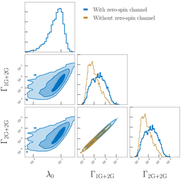
Figure 5: Posteriors of the inferred branching ratios, which are the relative 1G+2G vs. 1G+1G and 2G+2G vs. 1G+1G merger rates, and the fraction of 1G+1G binary black holes with zero-spin $\lambda_{0}$. In blue we plot the results when we allow for the zero-spin formation channel and in orange we plot the results when excluding the zero-spin formation channel (fixing $\lambda_{0}=0$).

As shown in Fig. 5, we find that the relative rates $\Gamma_{\textsf{1G+2G}}{}$ and $\Gamma_{\textsf{2G+2G}}{}$ are strongly correlated with the fraction $\lambda_{0}$ of 1G black holes that form in the zero-spin channel. These branching ratios are set by the fraction of 1G+1G merger products that are retained in a typical cluster. Since merging binaries with non-spinning components experience lower recoil velocities than those with non-negligible spin, the inclusion of the zero-spin formation channel drastically affects the retention fraction in the globular cluster potential, and consequently the branching ratios.

We find the median relative rates $\Gamma_{\textsf{1G+2G}}{}$ and $\Gamma_{\textsf{2G+2G}}{}$ to be $2.5\times 10^{-3}$ and $3.1\times 10^{-6}$, respectively, with $99\%$ upper limits of $0.049$ and $1.2\times 10^{-3}$. Adopting a fiducial binary black hole merger rate of $\sim 50~{}\mathrm{Gpc^{-3}\,yr^{-1}}$ (Abbott et al., 2019b) as a 1G+1G merger rate (we do not explicitly infer the rate as part of our model) these $99\%$ upper limits would imply merger rates of $\lesssim 2.5~{}\mathrm{Gpc^{-3}\,yr^{-1}}$ for $\Gamma_{\textsf{1G+2G}}{}$ and $\lesssim 0.06~{}\mathrm{Gpc^{-3}\,yr^{-1}}$ for $\Gamma_{\textsf{2G+2G}}{}$. Rerunning our analysis without the zero-spin subcomponent, the median branching ratios $\Gamma_{\textsf{1G+2G}}{}{}$ and $\Gamma_{\textsf{2G+2G}}{}{}$ become $8.1\times 10^{-4}$ and $3.3\times 10^{-7}$, respectively, with $99\%$ upper limits of $0.018$ and $1.6\times 10^{-4}$.

As the rates are much lower, we are less likely to observe hierarchical mergers than when there are black holes with effectively zero spin. The sensitivity of the merger rates to spin could potentially enable us to place tight constraints on the spins of 1G black holes—which are difficult to measure directly from GW observations (Poisson & Will, 1995; Pürrer et al., 2016; Vitale et al., 2014; Abbott et al., 2019a)—through the constraints on the hierarchical merger rate.

The lower branching ratios inferred when excluding the zero-spin formation channel affect the shape of the overall multigenerational population, with little support for primary masses in the PPSN mass gap. In the top panel of Fig. 4, we plot the reweighted component mass posterior samples for the $10$ events in GWTC-1, with the population model excluding the zero-spin component as a prior. The reduced hierarchical merger rates lead to smaller support for masses above the upper mass cutoff, and the $90\%$ interval on the primary black hole mass for GW170729 tightens to $34$–$53M_{\odot}$. Without the zero-spin population subcomponent, the $90\%$ upper limit on 1G+1G primary black hole spin magnitude becomes $0.54$.

The inferred branching ratios are consistent with Monte Carlo modeling of binary black hole populations in globular clusters; in the most extreme case where all black holes are assumed to be born with zero spin, such modeling predicts $\approx 13\%$ ($1\%$) of merging binary black holes are 1G+2G (2G+2G) systems (Rodriguez et al., 2019). As the natal spins of black holes increase, the retention fractions and relative rates precipitously drop as the recoil kicks become stronger. Rodriguez et al. (2019) find that if black hole natal spins are assumed to be $\chi=0.5$, that the number of black holes with a 2G component drops to $\lesssim 1\%$ of the total population.

4.3 Odds ratios for the hierarchical merger scenario

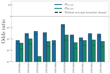
Figure 6: Hierarchical/1G+1G odds ratios for each of the GWTC-1 events. The odds for 1G+2G origin are plotted in blue, while the odds for 2G+2G origin are in green. The dashed lines indicate the odds when we use the model inferred when excluding the zero-spin channel. The dotted line indicates even odds.

With our multigenerational model, we also can calculate the hierarchical/1G+1G odds ratio $\mathcal{O}$ for each event. If the parameter distributions of each generational subpopulation were known, the odds ratio that the $i$-th observation came from a 1G+2G system versus a 1G+1G system would be

$$\mathcal{O}^{i}_{\textsf{1G+2G}}{}{}\equiv {}\>\frac{P(\textsf{1G+2G}{}|d_{i})}{P(\textsf{1G+1G}{}|d_{i})}$$

$$= {}\>\frac{Z(d_{i}|\textsf{1G+2G}{})}{Z(d_{i}|\textsf{1G+1G}{})}\frac{P(\textsf{1G+2G}{}{})}{P(\textsf{1G+1G}{}{})},$$ (34)

where the first term in Eq. (34) is the ratio of evidences for the observation given the 1G+2G and 1G+1G subpopulations (a Bayes factor; Kimball et al., 2020), and the second term is the prior odds (relative rates) of mergers of the two generations. However, as we do not know the exact form of the underlying population, our uncertainty in the population hyperparameters affects both the relative rates and the ratio of evidences. To take this into account, we marginalize over the population hyperparameters, weighting by our posterior probability distribution $p(\boldsymbol{\Lambda}|\vec{d})$, yielding

$$\mathcal{O}^{i}_{\textsf{1G+2G}}{}{}=\frac{\int\mathrm{d}\boldsymbol{\Lambda}Z(d_{i}|{\boldsymbol{\Lambda}},\textsf{1G+2G}{})\zeta_{\textsf{1G+2G}}{}{}(\boldsymbol{\Lambda})p(\boldsymbol{\Lambda}|\vec{d})}{\int\mathrm{d}\boldsymbol{\Lambda}Z(d_{i}|{\boldsymbol{\Lambda}},\textsf{1G+1G}{})\zeta_{\textsf{1G+1G}}{}{}(\boldsymbol{\Lambda})p(\boldsymbol{\Lambda}|\vec{d})}.$$ (35)

Here, the evidence for the 1G+2G population is

$$Z(d_{i}|{\boldsymbol{\Lambda}},\textsf{1G+2G}{})=\int\mathrm{d}\boldsymbol{\theta}L(d_{i}|\boldsymbol{\theta})\pi(\boldsymbol{\theta}|{\boldsymbol{\Lambda}},\textsf{1G+2G}{}),$$ (36)

while the 1G+1G evidence $Z(d_{i}|{\boldsymbol{\Lambda}},\textsf{1G+1G}{})$ is defined similarly, and $\zeta_{\textsf{1G+2G}}{}{}$ and $\zeta_{\textsf{1G+1G}}{}{}$ are the hierarchical merger fractions. The odds ratio for a 2G+2G system versus a 1G+1G system $\mathcal{O}^{i}_{\textsf{2G+2G}}{}{}$ can be calculated by swapping 1G+2G to 2G+2G in Eq. (35).

We calculate these odds ratios for all $10$ events in GWTC-1 (Abbott et al., 2019a), and plot the results in Fig. 6. For GW170729—the event with the most massive primary black hole—we favor a 1G+1G over a 1G+2G origin with $25$:$1$ odds when including the zero-spin formation channel. The probability that GW170729 is of hierarchical origin (either 1G+2G or 2G+2G) is $4\%$. GW151226, which has the most confidently measured non-zero spin (Abbott et al., 2016d, 2019a; Miller et al., 2020)—we find that $\log_{10}(Z_{\chi}/Z_{0})=6.5$—has the second highest probability ($0.2\%$) for a hierarchical origin. Across all $10$ systems in GWTC-1, we find the probability that at least one binary black hole system is of hierarchical origin is $5\%$.

As the inferred branching ratios are much smaller when excluding the zero-spin formation channel, the odds ratios for hierarchical origin in our globular cluster model, shown in dashed lines in Fig. 6, are reduced by $\sim 3$–$5$. If we exclude the zero-spin channel, we find that GW170729 most likely has a 1G+1G origin by a factor of $60$:$1$, and that the probability of at least one event being of hierarchical origin is only $2\%$.

The branching ratios are also dependent on the escape velocity of the dynamical environment. If we increase our cluster mass to $10^{8}$ $M_{\odot}$, typical of a nuclear star cluster, the branching ratios—and hence the odds ratios in favor of a hierarchical origin—increase by $\sim 1$–$3$ orders of magnitude. Since our transfer functions for 1G+2G and 2G+2G populations are tuned to globular cluster simulations, a robust analysis of an nuclear star cluster hierarchical merger scenario would require more detailed study.

To check how our prior on $m_{\mathrm{max}}$ affects our results we rerun the analysis with a uniform prior between $20M_{\odot}$ and $200M_{\odot}$. While we infer a peak in the posterior on $m_{\mathrm{max}}$ near $40M_{\odot}$, we find support all the way out to $200M_{\odot}$, well above any of the GWTC-1 black hole masses, indicating that we are insensitive to the existence of the mass gap (discussed further in Appendix A). The odds ratios in favor of the GWTC-1 events being hierarchical mergers remains largely the same, with a small increase in favor of hierarchical mergers as the prior for $m_{\mathrm{max}}$ extends down to $20M_{\odot}$. With this prior, the GW170729 1G+2G odds ratio is $0.041$. Allowing $m_{\mathrm{max}}$ to extend to larger values makes it easier to incorporate high-mass systems into the 1G+1G population. Cutting on the maximum of the $m_{\mathrm{max}}$ prior from $200M_{\odot}$ to $40M_{\odot}$ increases the GW170729 1G+2G odds ratio to $0.046$. Overall, our conclusions are not significantly affected by the prior assumptions on $m_{\mathrm{max}}$ as none of the systems lack posterior support for having masses below the PISN mass gap.

5 Conclusions

GW observations have demonstrated that binary black holes merge to form more massive black holes (Abbott et al., 2016a). If these merger products form a new binary, they may again become a GW source. The complete catalog of GW sources may therefore contain a mixture of 1G black holes formed from stellar collapse, and 2G black holes formed in mergers. In using the population of GW sources to infer the formation mechanisms for black holes, e.g., if their progenitors are subject to PPSN, it is necessary to account for the potential presence of 2G black holes to prevent our conclusions being biased. However, it is difficult to concretely distinguish between 1G and 2G black holes, as the populations overlap in properties. We perform an analysis that self-consistently infers both the fraction of binaries containing 2G black holes, and the fundamental properties of the population of 1G+1G binaries.

Our analysis uses phenomenological models to describe the binary black hole population. The models are calibrated to reproduce the features seen in simulations of globular clusters (Rodriguez et al., 2019). The fraction of 2G black holes that are retained in a cluster following a merger depends sensitively upon the spins of 1G black holes, as larger spins results in larger GW recoil kicks. Simulations of massive stars with efficient angular momentum transfer predict that black holes would form with spins $\lesssim 0.01$ (Fuller & Ma, 2019). Therefore, our population model also includes the possibility of a fraction of 1G black holes that have effectively zero spin. Our analysis demonstrates that this is a potentially key ingredient in the search for hierarchical mergers.

We apply our approach to the $10$ binary black holes found by LIGO and Virgo in their first two observing runs (Abbott et al., 2019a). We find that:

1. The 1G+1G population is fit by a steep power law with exponent $\alpha>0.83$ plus a Gaussian component with mean $\mu_{m}=31^{+7.1}_{-8.6}M_{\odot}$. We find an upper cutoff to the power law of $m_{\mathrm{max}}=47.5^{+16.5}_{-13.5}M_{\odot}$, but this is dominated by our choice of prior. Across the multigenerational population, we find that $99\%$ of black holes in binaries have masses $m_{1}\lesssim 45M_{\odot}$. Overall, the 1G+1G population is consistent with the mass distributions inferred in Abbott et al. (2019b).

2. The fraction of 1G+1G binaries with zero spin is $\lambda_{0}<0.32$ with $99\%$ probability, and $90\%$ of 1G+1G primary black holes have spins less than $0.57$. Excluding the zero-spin formation channel, $90\%$ of 1G+1G primary black holes have spins less than $0.54$

3. The median merger rates of 1G+2G and 2G+2G binaries relative to 1G+1G binaries are inferred to be $2.5\times 10^{-3}$ and $3.1\times 10^{-6}$, respectively, with $99\%$ upper limits of $0.049$ and $1.2\times 10^{-3}$. The relative rates are tightly correlated with the fraction of 1G black holes with zero spin. Excluding the zero-spin subcomponent of our spin distribution, the relative rates drop to $8.1\times 10^{-4}$ and $3.3\times 10^{-7}$ respectively, with $99\%$ upper limits of $0.018$ and $1.6\times 10^{-4}$. Since the relative rates and spins are tightly linked, a measurement of one would pin down the other.

4. The $10$ binary black holes from GWTC-1 are all consistent with being 1G+1G. Given the rarity of 1G+2G and 2G+2G mergers, this is not surprising. GW170729’s source, which is the most massive of the observed systems, is still found to most likely have a first-generation origin. This result is not especially sensitive to the allowed range for $m_{\mathrm{max}}$, as the masses for GW170729 are consistent with being below the PISN gap.

We cannot make a definite conclusion about the presence of hierarchical mergers amongst this catalog of $10$ events.

The analysis is currently limited to considering binary black holes formed in globular clusters. In reality, we expect that binary black holes form in other environments as well. Black holes in the field are unlikely to undergo a hierarchical merger. On the other hand, those formed in a nuclear star cluster are much more likely to be retained and available to form hierarchical mergers due to their higher escape velocities (Antonini & Rasio, 2016; Antonini et al., 2019; Yang et al., 2019).

Including alternative channels is necessary for definitively identifying hierarchical mergers, as this and other evolutionary channels, such as stellar collisions in young stellar clusters (Di Carlo et al., 2019), growth in active galactic nucleus disks (McKernan et al., 2012), or consecutive mergers in quadruple systems (Fragione et al., 2020), can grow black holes to masses above the PISN cutoff. The rate at which these mass-gap black holes form merging binaries is highly uncertain. If these black holes merge, they would be (incorrectly) classified as hierarchical mergers within our globular cluster picture.

Our method can be extended to include additional subpopulations. This would require defining new models, for example, including an aligned-spin distribution, as detailed in Eq. (5), to model binaries formed via isolated evolution (Kalogera, 2000; Rodriguez et al., 2016b). Including more subpopulations adds parameters to the likelihood, Eq. (26). With only the $10$ binaries, a relatively simple model is prudent (Abbott et al., 2019b). However, this will change as the catalog grows with further observing runs (Vitale et al., 2017; Stevenson et al., 2017; Zevin et al., 2017; Talbot & Thrane, 2017).

The third observing run of LIGO and Virgo began in April 2019 and was suspended in March 2020. The first binary black hole detection of the third observing run has recently been announced: GW190412 (Abbott et al., 2020b), a system with an unequal component masses; in Appendix B, we examine how adding this new event to the GWTC-1 updates our results, again finding that all binaries are consistent with being 1G+1G. Full results from the third observing run are still to be announced. The fourth observing run, which will extend the global GW detector network to include KAGRA (Akutsu et al., 2019), is scheduled to start in mid 2021 (Abbott et al., 2020a). As we gather more observing time, and improve the sensitivity of the detector network, we expect the number of observations and the rate of discoveries to increase. With larger catalogs of events it will be possible to make more precise measurements of the population, and we will be able to determine whether hierarchical mergers play a significant role in the GW catalog. Furthermore, improvements in the detectors’ low-frequency sensitivity will improve their ability to detect higher-mass binaries (Abbott et al., 2017b). The next generation of ground-based detectors offers the opportunity to perform the same measurements across cosmic time (Kalogera et al., 2019). With the precise population measurements coming from larger catalogs we can infer the details of the physical processes that shape black hole formation; however, for these conclusions to be accurate, it is necessary to account for the population being a mix of both 1G black holes and the products of mergers.

Appendix A GWTC-1 hyperparameter distributions

Here we present the full sets of inferred population parameter $\boldsymbol{\Lambda}$ posteriors for our population models. In Fig. 7, we plot the parameters determining the mass distributions, as defined in Eq. (2) and Eq. (3), for our default model. In Fig. 8 we plot the equivalent mass population hyperparameters for the model excluding the zero-spin subcomponent, and in Fig. 9 we plot the mass population hyperparameters when we switch to using a uniform prior for $m_{\mathrm{max}}$. The results are largely consistent between model choices.

When using the astrophysically motivated prior for $m_{\mathrm{max}}$, the posterior closely follows the prior. The posterior on $m_{\mathrm{max}}$ is more restricted at smaller values of the power-law index $\alpha$: when the mass distribution is flatter we are more sensitive to the upper cutoff than when the distribution sharply decreases with mass and we can increase the upper cutoff with little consequence (Fishbach & Holz, 2017). When switching to the uniform prior on $m_{\mathrm{max}}$ we see the same qualitative behavior with varying $\alpha$. For steep power laws ($\alpha\gtrsim 2$), we are effectively insensitive to the existence of an upper cutoff, but for flatter power laws ($\alpha\lesssim 1$), the dearth of higher-mass black holes means that there is little posterior support for $m_{\mathrm{max}}\gtrsim 45M_{\odot}$.

The power-law index $\alpha$ has more support for higher ($\alpha\gtrsim 2$) values. Our posterior on $\alpha$ is truncated by our choice of prior. Abbott et al. (2019b) found that the posterior on $\alpha$ becomes uninformative at large values ($\alpha\gtrsim 4$), with all values matching equally well.

The Gaussian component of the mass spectrum has a mean well constrained between $\mu_{m}\simeq 22$–$38M_{\odot}$. The exception to this is when $\lambda_{m}\sim 0$, as then the Gaussian component is negligible and so can be positioned anywhere. There is a correlation between the width of the Gaussian component $\sigma_{m}$ and the mean (Talbot & Thrane, 2018), with smaller $\mu_{m}$ permissible when $\sigma_{m}$ is larger, as this enables the upper edge of the Gaussian to stay in place. The value of $\sigma_{m}$ is not well constrained by the current set of observations.

The posteriors for the minimum mass $m_{\mathrm{min}}$ are largely unconstrained. As the GW detectors are less sensitive to low-mass systems, it is more difficult to place constraints on this end of the distribution (Fishbach & Holz, 2017; Talbot & Thrane, 2018; Abbott et al., 2019b). The lower limit of the $m_{\mathrm{min}}$ distribution is set by our prior, and the upper limit is set by the least massive black hole amongst our observations.

The mass ratio is degenerate with the spin (Poisson & Will, 1995; Baird et al., 2013; Farr et al., 2016). Fixing spins to be zero breaks the mass–spin degeneracy results in a more equal mass ratio and a larger $m_{2}$ for a system of a given chirp mass. However, the inclusion of the zero-spin subcomponent makes little difference for our inferred mass ratio distribution, with the posterior for the power-law index $\beta_{q}$ being largely determined by our assumed prior.

In Fig. 10, we plot the parameters determining the spin distributions, as defined in Eq. (4), for our default model. In Fig. 11 we plot the equivalent spin population hyperparameters for the model with $\lambda_{0}=0$, and in Fig. 12 we plot the spin population hyperparameters when using a uniform prior for $m_{\mathrm{max}}$. The $m_{\mathrm{max}}$ prior makes negligible difference to the spin distributions. There is no simple correlation between the fraction of 1G+1G binaries with zero spin $\lambda_{0}$ and the other population hyperparameters. The $\lambda_{0}$ distribution is peaked at $0$ and shows that many 1G+1G binaries are not well described by both black holes having near-zero spins. In all cases we favor models with $\alpha_{\chi}<\beta_{\chi}$, which corresponds to distributions which decrease with increasing spin magnitude (Farr et al., 2017; Abbott et al., 2019b).

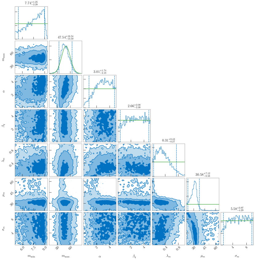
Figure 7: Posterior distributions of the population hyperparameters governing the mass and mass ratio distributions, when we allow a fraction of 1G black holes to form in the zero-spin channel. The dashed lines give the $90\%$ credible intervals, and the green lines indicate the priors.

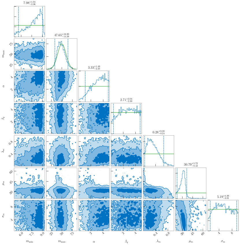
Figure 8: Inferred posterior distributions of the population hyperparameters governing the mass and mass ratio distributions when excluding the zero-spin formation channel. The dashed lines give the $90\%$ credible intervals intervals, and the green lines indicate the priors.

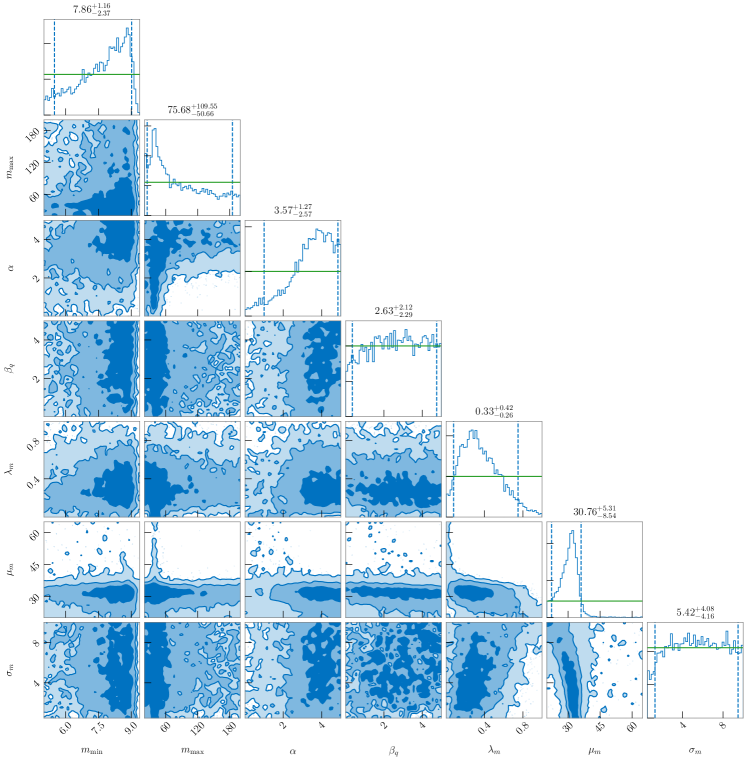
Figure 9: Posterior distributions of the population hyperparameters governing the mass distributions when we assume a flat prior on $m_{\mathrm{max}}$ The dashed lines give the $90\%$ credible intervals intervals, and the green lines indicate the priors.

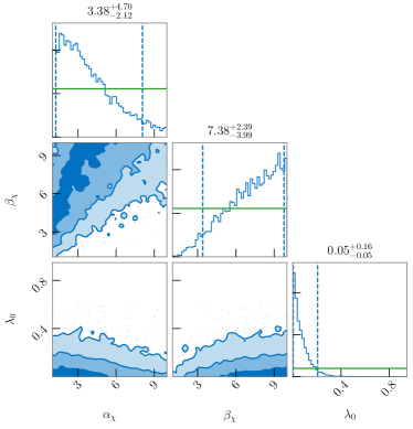
Figure 10: Posterior distributions of the population hyperparameters governing the spin distributions, when we allow a fraction of 1G black holes to form in the zero-spin channel. The dashed lines give the $90\%$ credible intervals intervals, and the green lines indicate the priors.

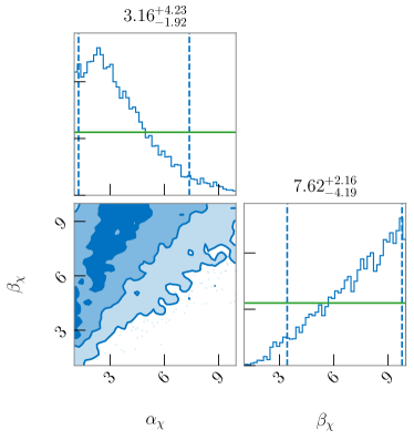
Figure 11: Posterior distributions of the population hyperparameters governing the spin distributions when excluding the zero-spin formation channel. The dashed lines give the $90\%$ credible intervals intervals, and the green lines indicate the priors.

Figure 12: Posterior distributions of the population hyperparameters governing the spin distributions when we assume a flat prior on $m_{\mathrm{max}}$ The dashed lines give the $90\%$ credible intervals intervals, and the green lines indicate the priors.

Appendix B Including GW190412

GW190412 is the first announced binary black hole detection of the third observing run of LIGO and Virgo (Abbott et al., 2020b). It is exceptional on account of its mass ratio, which is inferred as $q=0.28^{+0.13}_{-0.06}$ assuming the fiducial parameter estimation prior. The large difference in component masses would not be surprising for a hierarchical merger (Rodriguez et al., 2020; Gerosa et al., 2020), so here we investigate how our results change including GW190412. For this, we use parameter-estimation results for GW190412 from Zevin et al. (2020). Since GW190412 has been especially selected for publication, we cannot assume that using GWTC-1 plus GW190412 is a fair representation of the binary black hole population, and so results using these $11$ systems should be considered as preliminary, pending the completion of the catalog from the third observing run.

In Fig. 13, we plot the population hyperparameters for the mass and mass ratio distributions. As in Abbott et al. (2020b), we find that including GW190412 leads to tighter constraints on the mass ratio distribution. This single additional event acts as a lever arm, constraining $\beta_{q}$ to smaller values, flattening our inferred mass ratio distribution. The inferred spin parameters, shown in Fig. 14, are unaffected.

In Fig. 15, we show the odds ratios for our events having a hierarchical versus 1G+1G origin. The extreme mass ratio of GW190412 is well explained by the 1G+2G population, but its primary component’s spin is below the 2G black hole spin distribution. Overall, we find that GW190412 most likely has a 1G+1G origin, at odds of $\sim 500$:$1$. Including GW190412 also reduces the odds of GW170729 having a 1G+2G origin by $\sim 20\%$, since our 1G+1G mass ratio distribution flattens and has increased support at more unequal mass ratios. When we increase our cluster mass to $10^{8}M_{\odot}$, chosen to be typical of a nuclear star cluster, we still find that GW190412 most likely has a 1G+1G origin, but at lower odds of $\sim 6$:$1$.

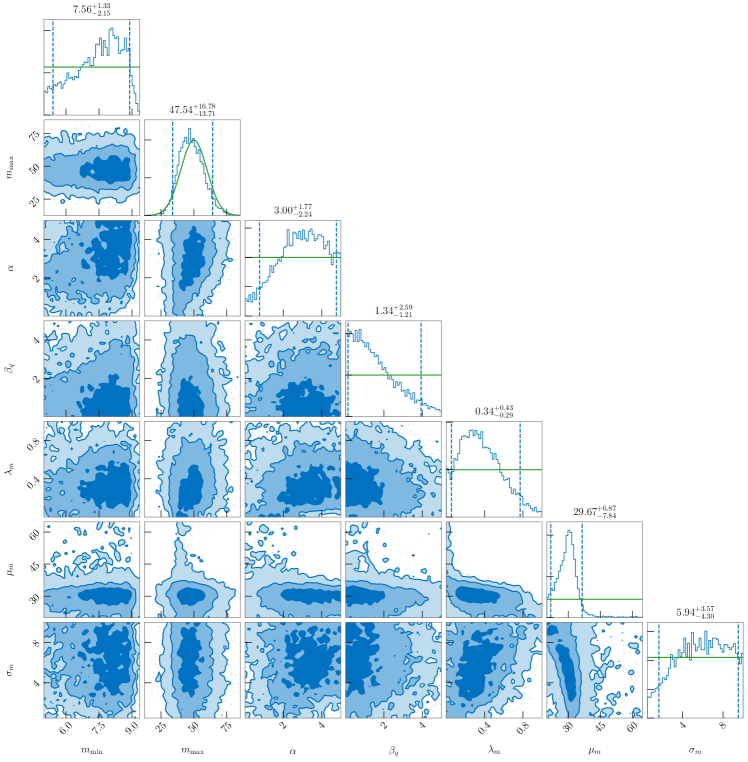
Figure 13: Posterior distributions of the population hyperparameters governing the mass and mass ratio distributions when we include GW190412, inferred with our model that allows a fraction of 1G black holes to form in the zero-spin channel. The dashed lines give the $90\%$ credible intervals, and the green lines indicate the priors.

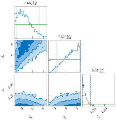
Figure 14: Posterior distributions of the population hyperparameters governing the spin distributions when we include GW190412, and allow a fraction of 1G black holes to form in the zero-spin channel. The dashed lines give the $90\%$ credible intervals intervals, and the green lines indicate the priors.

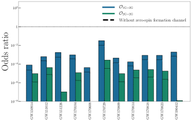
Figure 15: Hierarchical/1G+1G odds ratios for each of the GWTC-1 events as well as GW190412. The odds for a 1G+2G origin are plotted in blue, while the odds for a 2G+2G origin are in green. The dashed lines indicate the odds when we use the model inferred when excluding the zero-spin channel. The dotted line indicates even odds.

References

- Aasi et al. (2015) Aasi, J., et al. 2015, Class. Quant. Grav., 32, 074001
- Abbott et al. (2016a) Abbott, B. P., et al. 2016a, Phys. Rev. Lett., 116, 061102
- Abbott et al. (2016b) —. 2016b, Astrophys. J., 818, L22
- Abbott et al. (2016c) —. 2016c, Phys. Rev. Lett., 116, 241102
- Abbott et al. (2016d) —. 2016d, Phys. Rev. Lett., 116, 241103
- Abbott et al. (2017a) —. 2017a, Phys. Rev. Lett., 118, 221101, [Erratum: Phys. Rev. Lett.121,no.12,129901(2018)]
- Abbott et al. (2017b) —. 2017b, Phys. Rev., D96, 022001
- Abbott et al. (2019a) —. 2019a, Phys. Rev., X9, 031040
- Abbott et al. (2019b) —. 2019b, Astrophys. J., 882, L24
- Abbott et al. (2020a) —. 2020a, arXiv:1304.0670v10
- Abbott et al. (2019c) Abbott, R., et al. 2019c, arXiv:1912.11716
- Abbott et al. (2020b) —. 2020b, arXiv:2004.08342
- Abbott et al. (2020c) —. 2020c, Astrophys. J., 896, L44
- Acernese et al. (2015) Acernese, F., et al. 2015, Class. Quant. Grav., 32, 024001
- Akutsu et al. (2019) Akutsu, T., et al. 2019, Nat. Astron., 3, 35
- Antonini et al. (2019) Antonini, F., Gieles, M., & Gualandris, A. 2019, Mon. Not. Roy. Astron. Soc., 486, 5008
- Antonini & Rasio (2016) Antonini, F., & Rasio, F. A. 2016, Astrophys. J., 831, 187
- Arca Sedda et al. (2020) Arca Sedda, M., Mapelli, M., Spera, M., Benacquista, M., & Giacobbo, N. 2020, arXiv:2003.07409
- Ashton et al. (2019) Ashton, G., et al. 2019, Astrophys. J. Suppl., 241, 27
- Baibhav et al. (2020) Baibhav, V., Gerosa, D., Berti, E., et al. 2020, arXiv:2004.00650
- Baird et al. (2013) Baird, E., Fairhurst, S., Hannam, M., & Murphy, P. 2013, Phys. Rev., D87, 024035
- Banerjee (2020) Banerjee, S. 2020, arXiv:2004.07382
- Banerjee et al. (2010) Banerjee, S., Baumgardt, H., & Kroupa, P. 2010, Mon. Not. Roy. Astron. Soc., 402, 371
- Barkat et al. (1967) Barkat, Z., Rakavy, G., & Sack, N. 1967, Phys. Rev. Lett., 18, 379
- Barrett et al. (2018) Barrett, J. W., Gaebel, S. M., Neijssel, C. J., et al. 2018, Mon. Not. Roy. Astron. Soc., 477, 4685
- Belczynski et al. (2010) Belczynski, K., Dominik, M., Bulik, T., et al. 2010, Astrophys. J., 715, L138
- Belczynski et al. (2016) Belczynski, K., et al. 2016, Astron. Astrophys., 594, A97
- Belczynski et al. (2020) —. 2020, Astron. Astrophys., 636, A104
- Blanchet (2014) Blanchet, L. 2014, Living Rev. Rel., 17, 2
- Bruegmann et al. (2008) Bruegmann, B., Gonzalez, J. A., Hannam, M., Husa, S., & Sperhake, U. 2008, Phys. Rev., D77, 124047
- Buonanno et al. (2008) Buonanno, A., Kidder, L. E., & Lehner, L. 2008, Phys. Rev., D77, 026004
- Campanelli et al. (2007) Campanelli, M., Lousto, C. O., Zlochower, Y., & Merritt, D. 2007, Astrophys. J., 659, L5
- Chatziioannou et al. (2019) Chatziioannou, K., et al. 2019, Phys. Rev., D100, 104015
- Cutler & Flanagan (1994) Cutler, C., & Flanagan, E. E. 1994, Phys. Rev., D49, 2658
- Di Carlo et al. (2019) Di Carlo, U. N., Mapelli, M., Bouffanais, Y., et al. 2019, arXiv:1911.01434
- Doctor et al. (2019) Doctor, Z., Wysocki, D., O’Shaughnessy, R., Holz, D. E., & Farr, B. 2019, arXiv:1911.04424
- Downing et al. (2011) Downing, J. M. B., Benacquista, M. J., Giersz, M., & Spurzem, R. 2011, Mon. Not. Roy. Astron. Soc., 416, 133
- Ertl et al. (2020) Ertl, T., Woosley, S. E., Sukhbold, T., & Janka, H. T. 2020, Astrophys. J., 890, 51
- Farmer et al. (2019) Farmer, R., Renzo, M., de Mink, S. E., Marchant, P., & Justham, S. 2019, Astrophys. J., 887, 53
- Farr et al. (2016) Farr, B., et al. 2016, Astrophys. J., 825, 116
- Farr et al. (2019) Farr, W. M., Fishbach, M., Ye, J., & Holz, D. 2019, Astrophys. J. Lett., 883, L42
- Farr et al. (2017) Farr, W. M., Stevenson, S., Coleman Miller, M., et al. 2017, Nature, 548, 426
- Finn & Chernoff (1993) Finn, L. S., & Chernoff, D. F. 1993, Phys. Rev., D47, 2198
- Fishbach & Holz (2017) Fishbach, M., & Holz, D. E. 2017, Astrophys. J., 851, L25
- Fishbach et al. (2017) Fishbach, M., Holz, D. E., & Farr, B. 2017, Astrophys. J., 840, L24
- Fowler & Hoyle (1964) Fowler, W. A., & Hoyle, F. 1964, Astrophys. J. Suppl., 9, 201
- Fragione et al. (2020) Fragione, G., Loeb, A., & Rasio, F. A. 2020, arXiv:2002.11278
- Fryer et al. (2001) Fryer, C. L., Woosley, S. E., & Heger, A. 2001, Astrophys. J., 550, 372
- Fuller & Ma (2019) Fuller, J., & Ma, L. 2019, Astrophys. J., 881, L1
- Gerosa & Berti (2017) Gerosa, D., & Berti, E. 2017, Phys. Rev., D95, 124046
- Gerosa & Berti (2019) —. 2019, Phys. Rev., D100, 041301
- Gerosa & Kesden (2016) Gerosa, D., & Kesden, M. 2016, Phys. Rev., D93, 124066
- Gerosa et al. (2020) Gerosa, D., Vitale, S., & Berti, E. 2020, arXiv:2005.04243
- Gonzalez et al. (2007) Gonzalez, J. A., Sperhake, U., Bruegmann, B., Hannam, M., & Husa, S. 2007, Phys. Rev. Lett., 98, 091101
- Healy et al. (2014) Healy, J., Lousto, C. O., & Zlochower, Y. 2014, Phys. Rev., D90, 104004
- Heger et al. (2003) Heger, A., Fryer, C. L., Woosley, S. E., Langer, N., & Hartmann, D. H. 2003, Astrophys. J., 591, 288
- Heger & Woosley (2002) Heger, A., & Woosley, S. E. 2002, Astrophys. J., 567, 532
- Heggie (1975) Heggie, D. C. 1975, Mon. Not. Roy. Astron. Soc., 173, 729
- Heggie et al. (1996) Heggie, D. C., Hut, P., & McMillan, S. L. W. 1996, ApJ, 467, 359
- Jiménez-Forteza et al. (2017) Jiménez-Forteza, X., Keitel, D., Husa, S., et al. 2017, Phys. Rev., D95, 064024
- Kalogera (2000) Kalogera, V. 2000, Astrophys. J., 541, 319
- Kalogera et al. (2019) Kalogera, V., et al. 2019, Bull. Am. Astron. Soc, 51, 242
- Kimball et al. (2020) Kimball, C., Berry, C. P. L., & Kalogera, V. 2020, R. Notes AAS, 4, 2
- Kruckow et al. (2018) Kruckow, M. U., Tauris, T. M., Langer, N., Kramer, M., & Izzard, R. G. 2018, Mon. Not. Roy. Astron. Soc., 481, 1908
- Lousto & Zlochower (2011) Lousto, C. O., & Zlochower, Y. 2011, Phys. Rev. Lett., 107, 231102
- Mandel & Farmer (2018) Mandel, I., & Farmer, A. 2018, arXiv:1806.05820
- Mandel et al. (2019) Mandel, I., Farr, W. M., & Gair, J. R. 2019, Mon. Not. Roy. Astron. Soc., 486, 1086
- Mapelli et al. (2020) Mapelli, M., Spera, M., Montanari, E., et al. 2020, Astrophys. J., 888, 376
- Marchant et al. (2019) Marchant, P., Renzo, M., Farmer, R., et al. 2019, Astrophys. J., 882, 36
- McKernan et al. (2012) McKernan, B., Ford, K. E. S., Lyra, W., & Perets, H. B. 2012, Mon. Not. Roy. Astron. Soc., 425, 460
- Merritt et al. (2004) Merritt, D., Milosavljevic, M., Favata, M., Hughes, S. A., & Holz, D. E. 2004, Astrophys. J., 607, L9
- Miller & Hamilton (2002) Miller, M. C., & Hamilton, D. P. 2002, Astrophys. J., 576, 894
- Miller & Miller (2014) Miller, M. C., & Miller, J. M. 2014, Phys. Rept., 548, 1
- Miller et al. (2020) Miller, S., Callister, T. A., & Farr, W. 2020, arXiv:2001.06051
- Moody & Sigurdsson (2009) Moody, K., & Sigurdsson, S. 2009, Astrophys. J., 690, 1370
- Neijssel et al. (2019) Neijssel, C. J., Vigna-Gómez, A., Stevenson, S., et al. 2019, Mon. Not. Roy. Astron. Soc., 490, 3740
- Nitz et al. (2020) Nitz, A. H., Dent, T., Davies, G. S., et al. 2020, Astrophys. J., 891, 123
- Plummer (1911) Plummer, H. C. 1911, Mon. Not. Roy. Astron. Soc., 71, 460
- Poisson & Will (1995) Poisson, E., & Will, C. M. 1995, Phys. Rev., D52, 848
- Portegies Zwart & McMillan (2000) Portegies Zwart, S. F., & McMillan, S. 2000, Astrophys. J., 528, L17
- Pretorius (2005) Pretorius, F. 2005, Phys. Rev. Lett., 95, 121101
- Pürrer et al. (2016) Pürrer, M., Hannam, M., & Ohme, F. 2016, Phys. Rev., D93, 084042
- Qin et al. (2018) Qin, Y., Fragos, T., Meynet, G., et al. 2018, Astron. Astrophys., 616, A28, [Astron. Astrophys.616,A28(2018)]
- Reisswig et al. (2009) Reisswig, C., Husa, S., Rezzolla, L., et al. 2009, Phys. Rev., D80, 124026
- Rodriguez et al. (2018) Rodriguez, C. L., Amaro-Seoane, P., Chatterjee, S., & Rasio, F. A. 2018, Phys. Rev. Lett., 120, 151101
- Rodriguez et al. (2016a) Rodriguez, C. L., Chatterjee, S., & Rasio, F. A. 2016a, Phys. Rev., D93, 084029
- Rodriguez et al. (2019) Rodriguez, C. L., Zevin, M., Amaro-Seoane, P., et al. 2019, Phys. Rev., D100, 043027
- Rodriguez et al. (2016b) Rodriguez, C. L., Zevin, M., Pankow, C., Kalogera, V., & Rasio, F. A. 2016b, Astrophys. J., 832, L2
- Rodriguez et al. (2020) Rodriguez, C. L., et al. 2020, arXiv:2005.04239
- Romero-Shaw et al. (2020) Romero-Shaw, I. M., et al. 2020, arXiv:2006.00714
- Sigurdsson & Phinney (1993) Sigurdsson, S., & Phinney, E. S. 1993, ApJ, 415, 631
- Speagle (2020) Speagle, J. S. 2020, Mon. Not. Roy. Astron. Soc., 493, 3132
- Spera & Mapelli (2017) Spera, M., & Mapelli, M. 2017, Mon. Not. Roy. Astron. Soc., 470, 4739
- Spera et al. (2015) Spera, M., Mapelli, M., & Bressan, A. 2015, Mon. Not. Roy. Astron. Soc., 451, 4086
- Sperhake (2015) Sperhake, U. 2015, Class. Quant. Grav., 32, 124011
- Stevenson et al. (2017) Stevenson, S., Berry, C. P. L., & Mandel, I. 2017, Mon. Not. Roy. Astron. Soc., 471, 2801
- Stevenson et al. (2015) Stevenson, S., Ohme, F., & Fairhurst, S. 2015, Astrophys. J., 810, 58
- Stevenson et al. (2019) Stevenson, S., Sampson, M., Powell, J., et al. 2019, Astrophys. J., 882, 121
- Talbot et al. (2019) Talbot, C., Smith, R., Thrane, E., & Poole, G. B. 2019, Phys. Rev., D100, 043030
- Talbot & Thrane (2017) Talbot, C., & Thrane, E. 2017, Phys. Rev., D96, 023012
- Talbot & Thrane (2018) —. 2018, Astrophys. J., 856, 173
- Thrane & Talbot (2019) Thrane, E., & Talbot, C. 2019, Publ. Astron. Soc. Austral., 36, e010
- van Son et al. (2020) van Son, L. A. C., de Mink, S. E., Broekgaarden, F. S., et al. 2020, arXiv:2004.05187
- Varma et al. (2019) Varma, V., Gerosa, D., Stein, L. C., Hébert, F., & Zhang, H. 2019, Phys. Rev. Lett., 122, 011101
- Varma et al. (2020) Varma, V., Isi, M., & Biscoveanu, S. 2020, arXiv:2002.00296
- Venumadhav et al. (2019) Venumadhav, T., Zackay, B., Roulet, J., Dai, L., & Zaldarriaga, M. 2019, Phys. Rev., D100, 023011
- Venumadhav et al. (2020) —. 2020, Phys. Rev., D101, 083030
- Vitale et al. (2017) Vitale, S., Lynch, R., Sturani, R., & Graff, P. 2017, Class. Quant. Grav., 34, 03LT01
- Vitale et al. (2014) Vitale, S., Lynch, R., Veitch, J., Raymond, V., & Sturani, R. 2014, Phys. Rev. Lett., 112, 251101
- Woosley (2017) Woosley, S. E. 2017, Astrophys. J., 836, 244
- Woosley et al. (2007) Woosley, S. E., Blinnikov, S., & Heger, A. 2007, Nature, 450, 390
- Woosley & Heger (2015) Woosley, S. E., & Heger, A. 2015, Astrophys. Space Sci. Libr., 412, 199
- Woosley et al. (2002) Woosley, S. E., Heger, A., & Weaver, T. A. 2002, Rev. Mod. Phys., 74, 1015
- Wysocki et al. (2019) Wysocki, D., Lange, J., & O’Shaughnessy, R. 2019, Phys. Rev., D100, 043012
- Yang et al. (2019) Yang, Y., et al. 2019, Phys. Rev. Lett., 123, 181101
- Zackay et al. (2019a) Zackay, B., Dai, L., Venumadhav, T., Roulet, J., & Zaldarriaga, M. 2019a, arXiv:1910.09528
- Zackay et al. (2019b) Zackay, B., Venumadhav, T., Dai, L., Roulet, J., & Zaldarriaga, M. 2019b, Phys. Rev., D100, 023007
- Zevin et al. (2020) Zevin, M., Berry, C. P. L., Coughlin, S., Chatziioannou, K., & Vitale, S. 2020, arXiv:2006.11293
- Zevin et al. (2017) Zevin, M., Pankow, C., Rodriguez, C. L., et al. 2017, Astrophys. J., 846, 82