DESY-20-059, TTP-2020-017, P3H-20-013
Phenomenology of a Supersymmetric Model Inspired by Inflation

Abstract

The current challenges in High Energy Physics and Cosmology are to build coherent particle physics models to describe the phenomenology at colliders in the laboratory and the observations in the universe. From these observations, the existence of an inflationary phase in the early universe gives guidance for particle physics models. We study a supersymmetric model which incorporates successfully inflation by a non-minimal coupling to supergravity and shows a unique collider phenomenology. Motivated by experimental data, we set a special emphasis on a new singlet-like state at $97\,\textrm{GeV}$ and single out possible observables for a future linear collider that permit a distinction of the model from a similar scenario without inflation. We define a benchmark scenario that is in agreement with current collider and Dark Matter constraints, and study the influence of the non-minimal coupling on the phenomenology. Measuring the singlet-like state with high precision on the percent level seems to be promising for resolving the models, even though the Standard Model-like Higgs couplings deviate only marginally. However, a hypothetical singlet-like state with couplings of about $20\,\%$ compared to a Standard Model Higgs at $97\,\textrm{GeV}$ encourages further studies of such footprint scenarios of inflation.

 

1 Introduction

Supersymmetry (SUSY) remains a valid conceptual extension beyond the Standard Model (SM) of particle physics, although there have not yet been any direct signs of superpartners detected in proton–proton collisions even at 13 TeV center of mass energy at the run 2 of the Large Hadron Collider (LHC). Nevertheless, light SUSY states from the electroweak sector cannot be excluded, not even at relatively low masses. The concept of SUSY as a space-time symmetry is mathematically sound, phenomenologically beautiful and connects the fundamental forces of the SM with gravity. In supergravity, moreover, a non-minimal gravitational coupling of the Higgs particle content leads to a successful embedding of inflation in the early universe [1, 2, 3, 4]. The basic Higgs phenomenology of this variation of a Next-to-Minimal Supersymmetric Standard Model (NMSSM) has been described in some detail in [5], where it has been argued, that the main effect of the non-minimal supergravity coupling might be visible in a precise study of a singlet-like Higgs state that has to be discovered at the LHC or future lepton colliders.

Especially the option of a light additional Higgs state at $97\,\textrm{GeV}$ as favoured by some observational hints at the Large Electron–Positron Collider (LEP) [6, 7, 8] and the LHC [9, 10, 11], which can be present in many singlet extended models [12, 13, 14, 15, 16, 17, 18, 19, 20, 21, 22, 23, 24], is an intriguing case study also for the inflation-inspired model. We want to state that the existence or nonexistence of such a light Higgs is neither unique to the model which is going to be studied in the current work, nor is it a special feature of it. However, it is interesting to connect to new light bosons as they could be studied with unprecedented precision in future $e^{+}e^{-}$-colliders, for instance at the International Linear Collider (ILC) with an initial low center of mass energy of $250\,\textrm{GeV}$. Thus, we are going to put special emphasis on the $e^{+}e^{-}$-collider phenomenology of a benchmark point which comprises such a scalar boson below $100\,\textrm{GeV}$.

This paper is structured as follows: first, we briefly review the supersymmetric model motivated by inflation in Sec. 2 which has been introduced in Refs. [2, 3]. The phenomenology of the the Higgs and of the electroweakino sector has already been discussed in detail in Ref. [5] to which we closely relate here. Second, we perfom a scan of the relevant model parameters from which we extract a benchmark scenario which is discussed in more detail in Sec. 3 and discuss the phenomenology of such a scenario. Finally, our conclusions are presented in Sec. 4.

2 Theoretical Framework

The model with successful early universe inflation in the context of superconformal supergravity [2, 3, 4] can be embedded in the general NMSSM (GNMSSM) as reviewed in Ref. [26]. In order to drive inflation, a non-minimal coupling of a Higgs bilinear to gravity is needed, which has been shown to be the gauge invariant product $\hat{H}_{u}\cdot\hat{H}_{d}$, as pointed out in Ref. [1]. The singlet superfield is needed to stabilise the inflationary direction [2, 3, 4]. At low (electroweak) energies, the superpotential is given by the superpotential of the $\mathbb{Z}_{3}$-invariant NMSSM plus an additional $\mu$-term like in the Minimal Supersymmetric Standard Model (MSSM) $\mu\,\hat{H}_{u}\cdot\hat{H}_{d}$. This parameter we name for clarity $\mu_{\text{inf}}$ and the model thus “$\mu$-extended” NMSSM or short $\mu$NMSSM. In contrast to the $\mathbb{Z}_{3}$-invariant NMSSM, there is no accidental $\mathbb{Z}_{3}$ symmetry prohibiting certain terms in the superpotential of the GNMSSM like the $\mu$-term for the two Higgs doublet superfields and the mass and tadpole term for the singlet superfield. The $\mu$-term breaks the $\mathbb{Z}_{3}$ symmetry of the NMSSM and thus also non-$\mathbb{Z}_{3}$-invariant terms in the soft SUSY breaking sector are supposed to be present. Nevertheless, due to breaking of the superconformal symmetry by only the gravitational coupling, the superpotential does not introduce the mass and tadpole term for the singlet. The soft breaking terms can always be redefined in a way that only the couplings introduced below are relevant.

The superpotential of the $\mu$NMSSM is given by

$$\mathcal{W}_{\mu\text{NMSSM}}= (\lambda\hat{S}+\mu_{\text{inf}})\hat{H}_{u}\cdot\hat{H}_{d}+\frac{\kappa}{3}\hat{S}^{3}+\mathcal{W}_{\text{Yukawa}}\,,$$ (1)

where the extra $\mu$-term is related to the non-minimal supergravity coupling $\chi$ via the gravitino mass as $\mu_{\text{inf}}=\frac{3}{2}m_{3/2}\chi$. The Yukawa terms are the same as in the (N)MSSM. Chiral superfields are denoted with a hat, where $\hat{H}_{u}$ and $\hat{H}_{d}$ are the up- and down-type Higgs doublet, respectively, and $\hat{S}$ the singlet superfield. The corresponding soft SUSY breaking Lagrangian is given by

$$\begin{split}-\mathcal{L}_{\text{soft}}&=\left[A_{\lambda}\,\lambda\,S\,H_{u}\cdot H_{d}+\frac{1}{3}\,A_{\kappa}\,\kappa\,S^{3}+B_{\mu}\,\mu\,H_{u}\cdot H_{d}+\text{h.\,c.}\right]\\ &\quad+m_{H_{d}}^{2}\,\lvert H_{d}\rvert^{2}+m_{H_{u}}^{2}\,\lvert H_{u}\rvert^{2}+m_{s}^{2}\,\lvert S\rvert^{2}\,.\end{split}$$ (2)

The soft SUSY breaking Higgs masses can be related to the electroweak symmetry breaking conditions and are no free parameters. The $B_{\mu}$ terms play a subdominant role and can be set to zero throughout this work.

After electroweak symmetry breaking, the scalar components of the three Higgs superfields acquire vacuum expectation values (vevs) $v_{u}$, $v_{d}$ and $v_{s}$. We expand these fields around the vacuum configuration and write:

$$H_{u}=\begin{pmatrix}h_{u}^{+}\\ h_{u}\end{pmatrix}=\begin{pmatrix}\eta_{u}^{+}\\ v_{u}+\frac{1}{\sqrt{2}}(\sigma_{u}+i\phi_{u})\end{pmatrix},\quad H_{d}=\begin{pmatrix}h_{d}\\ h_{d}^{-}\end{pmatrix}=\begin{pmatrix}v_{d}+\frac{1}{\sqrt{2}}(\sigma_{d}+i\phi_{d})\\ \eta_{d}^{-}\end{pmatrix}$$

$$S=v_{s}+\frac{1}{\sqrt{2}}(\sigma_{s}+i\phi_{s}).$$ (3)

The ratio of the two doublet vevs defines the parameter $\tan\beta=v_{u}/v_{d}$, where $v=\sqrt{v_{u}^{2}+v_{d}^{2}}=174\,\textrm{GeV}$ corresponds to the SM-vev. Consequently, $v_{u}$ and $v_{d}$ are given by $v_{u}=v\sin\beta$ and $v_{d}=v\cos\beta$. The vev of the singlet field $S$ dynamically induces a $\mu$-term which we denote as the effective $\mu$-term, $\mu_{\text{eff}}=\lambda v_{s}$. Although it might be suggestive to combine the two $\mu$-terms as $\mu_{\text{eff}}\to\mu_{\text{inf}}+\mu_{\text{eff}}$, they lead to different phenomenologies in the Higgs and Neutralino sector, as has been pointed out in Ref. [5].

Thus, we consider both $\mu_{\text{inf}}$ and $\mu_{\text{eff}}$ as independent free parameters in our study. The consequent differences in the phenomenology will be the crucial point of our discussion. The Neutralino–Singlino mixing will also be affected by the interplay of $\mu_{\text{inf}}$ and $\mu_{\text{eff}}$ and therewith the character of the contribution to dark matter may vary. Since $\mu_{\text{inf}}$ is related to the gravitino mass, dark matter might also be pure gravitino dark matter, see the discussion in Ref. [5].

According to the cosmological analysis [3, 4], the value of the non-minimal gravity coupling $\chi$ can be estimated to $\chi\simeq 10^{5}\lambda$. Thus, with $\lambda>0$, we also set $\mu_{\text{inf}}$ to be non-negative.

2.1 Higgs sector

The superpotential (1) and the soft-breaking Lagrangian (2) together with the usual $D$-terms (quartic Higgs couplings due to quadratic gauge couplings which do not exist for the singlet) lead to the following scalar Higgs potential (with $B_{\mu}=0$):

$$V_{\text{Higgs}}=\; \left(m_{H_{d}}^{2}+(\mu_{\text{inf}}+\lambda S)^{2}\right)|H_{d}|^{2}+\left(m_{H_{u}}^{2}+(\mu_{\text{inf}}+\lambda S)^{2}\right)|H_{u}|^{2}$$

$$\;+\left(\kappa S^{2}+\lambda H_{u}\cdot H_{d}\right)^{2}+\frac{g_{2}^{2}}{2}|H_{d}^{\dagger}H_{u}|^{2}+\frac{g_{1}^{2}+g_{2}^{2}}{8}\left(|H_{d}|^{2}-|H_{u}|^{2}\right)^{2}$$

$$\;+m_{S}^{2}S^{2}+2\lambda A_{\lambda}SH_{u}\cdot H_{d}+\frac{2}{3}\kappa A_{\kappa}S^{3}\,.$$ (4)

The mass terms finally arise from the second derivative with respect to the component fields in Eqs. (2) evaluated at the vacuum. Note that the soft breaking terms $m_{H_{u}}^{2}$, $m_{H_{d}}^{2}$ and $m_{S}^{2}$ are fixed by the minimisation conditions for electroweak symmetry breaking. For convenience, we list the mass matrix elements of the scalar, pseudoscalar and charged Higgs matrices, $M_{S}^{2}$, $M_{P}^{2}$, and $M_{C}^{2}$, respectively, as worked out in Ref. [5]; we only keep the contribution from $\mu_{\text{inf}}$ in comparison with the GNMSSM:

$${M}_{S,11}^{2}=m_{Z}^{2}\cos^{2}\beta+\mu_{\text{eff}}\left(\frac{\kappa}{\lambda}\mu_{\text{eff}}+A_{\lambda}\right)\tan\beta$$ (5a)

$${M}_{S,22}^{2}=m_{Z}^{2}\sin^{2}\beta+\mu_{\text{eff}}\left(\frac{\kappa}{\lambda}\mu_{\text{eff}}+A_{\lambda}\right)/\tan\beta$$ (5b)

$${M}_{S,33}^{2}=\frac{\lambda^{2}v^{2}}{\mu_{\text{eff}}}(\cos\beta\sin\beta A_{\lambda}-\mu_{\text{inf}})+\frac{\kappa}{\lambda}\mu_{\text{eff}}\left(A_{\kappa}+4\frac{\kappa}{\lambda}\mu_{\text{eff}}\right)$$ (5c)

$${M}_{S,12}^{2}={M}_{S,21}^{2}=(2v^{2}\lambda^{2}-m_{Z}^{2})\cos\beta\sin\beta-\mu_{\text{eff}}\left(\frac{\kappa}{\lambda}\mu_{\text{eff}}+A_{\lambda}\right)$$ (5d)

$${M}_{S,13}^{2}={M}_{S,31}^{2}=\lambda v\left(2(\mu_{\text{eff}}+\mu_{\text{inf}})\cos\beta-\left(A_{\lambda}+2\frac{\kappa}{\lambda}\mu_{\text{eff}}\right)\sin\beta\right)$$ (5e)

$${M}_{S,23}^{2}={M}_{S,32}^{2}=\lambda v\left(2(\mu_{\text{eff}}+\mu_{\text{inf}})\sin\beta-\left(A_{\lambda}+2\frac{\kappa}{\lambda}\mu_{\text{eff}}\right)\cos\beta\right)\,,$$ (5f)

$${M}_{P,11}^{2}=\mu_{\text{eff}}\left(\frac{\kappa}{\lambda}\mu_{\text{eff}}+A_{\lambda}\right)\tan\beta$$ (6a)

$${M}_{P,22}^{2}=\mu_{\text{eff}}\left(\frac{\kappa}{\lambda}\mu_{\text{eff}}+A_{\lambda}\right)/\tan\beta$$ (6b)

$${M}_{P,33}^{2}=\frac{\lambda^{2}v^{2}}{\mu_{\text{eff}}}\Big{(}(4\frac{\kappa}{\lambda}\mu_{\text{eff}}+A_{\lambda})\cos\beta\sin\beta-\mu_{\text{inf}}\Big{)}-3\frac{\kappa}{\lambda}\mu_{\text{eff}}A_{\kappa}$$ (6c)

$${M}_{P,12}^{2}={M}_{P,21}^{2}=\mu_{\text{eff}}\left(\frac{\kappa}{\lambda}\mu_{\text{eff}}+A_{\lambda}\right)$$ (6d)

$${M}_{P,13}^{2}={M}_{P,31}^{2}=-v\lambda\left(2\frac{\kappa}{\lambda}\mu_{\text{eff}}-A_{\lambda}\right)\sin\beta$$ (6e)

$${M}_{P,23}^{2}={M}_{P,32}^{2}=-v\lambda\left(2\frac{\kappa}{\lambda}\mu_{\text{eff}}-A_{\lambda}\right)\cos\beta\,,$$ (6f)

$${M}_{C,11}^{2}=(m^{2}_{W}-v^{2}\lambda^{2})\sin^{2}\beta+\mu_{\text{eff}}\left(\frac{\kappa}{\lambda}\mu_{\text{eff}}+A_{\lambda}\right)\tan\beta$$ (7a)

$${M}_{C,22}^{2}=(m^{2}_{W}-v^{2}\lambda^{2})\cos^{2}\beta+\mu_{\text{eff}}\left(\frac{\kappa}{\lambda}\mu_{\text{eff}}+A_{\lambda}\right)/\tan\beta$$ (7b)

$${M}_{C,12}^{2}=(m^{2}_{W}-v^{2}\lambda^{2})\sin\beta\cos\beta+\mu_{\text{eff}}\left(\frac{\kappa}{\lambda}\mu_{\text{eff}}+A_{\lambda}\right)\,.$$ (7c)

The pseudoscalar and charged mass matrix comprise one vanishing eigenvalue each. These correspond to the would-be-Goldstone modes. Diagonalisation of those two matrices is easy and can be done with a rotation by the angle $\beta$. The charged Higgs mass is then found to be given by the expression:

$$m_{H^{\pm}}^{2}=m_{W}^{2}-v^{2}\lambda^{2}+\frac{\mu_{\text{eff}}}{\cos\beta\sin\beta}\left(\frac{\kappa}{\lambda}\mu_{\text{eff}}+A_{\lambda}\right)\,,$$ (8)

from which we can resolve for $A_{\lambda}$ and use $m_{H^{\pm}}$ as input parameter to replace the appearance of $A_{\lambda}$ in the model. We then can use the relation

$$\mu_{\text{eff}}\left(\frac{\kappa}{\lambda}\mu_{\text{eff}}+A_{\lambda}\right)=(m_{H^{\pm}}^{2}-m_{W}^{2}+v^{2}\lambda^{2})\cos\beta\sin\beta$$ (9)

to cancel out the $\kappa$ and $\mu_{\text{eff}}$ dependences in Eqs. (6f) and (7c). Furthermore, if we fix $m_{H^{\pm}}$ to a large value $m_{H^{\pm}}^{2}\gg v^{2}$, the heaviest neutral Higgs bosons both for CP-even and CP-odd case are basically independent of $\kappa$, $\mu_{\text{eff}}$ and $\mu_{\text{inf}}$; i. e. the heavy mass eigenvalues are dominantly controlled by $m_{H^{\pm}}$. We are in general left with the following free parameters in our study:

$$\tan\beta,\quad\lambda,\quad\kappa,\quad\mu_{\text{eff}},\quad\mu_{\text{inf}},\quad A_{\kappa},\quad m_{H^{\pm}}.$$ (10)

In the following, we treat both $\tan\beta$ and $m_{H^{\pm}}$ as fixed input parameters that are kept to some experimentally allowed value. By this choice, the matrix elements $M_{S,P,11}^{2}$, $M_{S,P,22}^{2}$ and $M_{S,P,12}^{2}$ do not vary under variation of the other inputs. We are interested in the effect of the inflation specific parameters, for which $\tan\beta$ and $m_{H^{\pm}}$ play a subleading role and have rather the same influence as in the usual NMSSM. The further elements $M_{S,P,13}^{2}$, $M_{S,P,23}^{2}$ and $M_{S,P,33}^{2}$ are then mainly controlled by the parameter combinations $\frac{\kappa}{\lambda}\mu_{\text{eff}}$ and the sum $\mu_{\text{eff}}+\mu_{\text{inf}}$ aside from $m_{H^{\pm}}$. Thus, the properties of the light neutral Higgs states at tree level are dominated by these two combinations, although the other free parameters $\lambda$, $A_{\kappa}$, and $\mu_{\text{inf}}$ can influence the mass matrices.

From the diagonalisation, we retrieve the Higgs mixing parameters $S_{ij}$, $P_{ij}$ and $C_{ij}$ for the scalar, pseudoscalar and charged cases, respectively. The diagonal matrices are found as $\boldsymbol{\tilde{M}}_{S}^{2}=\boldsymbol{S}^{\dagger}\boldsymbol{M}_{S}^{2}\boldsymbol{S}$, $\boldsymbol{\tilde{M}}_{P}^{2}=\boldsymbol{P}^{\dagger}\boldsymbol{M}_{P}^{2}\boldsymbol{P}$, and $\boldsymbol{\tilde{M}}_{C}^{2}=\boldsymbol{C}^{\dagger}\boldsymbol{M}_{C}^{2}\boldsymbol{C}$. With the mixing matrices, the Higgs couplings to SM particles can be conveniently expressed and compared to the SM values in terms of “reduced” couplings. So for example, reduced couplings of the $i$-th scalar Higgs to bottom and top quarks are given by:

$$\frac{g_{h_{i}b\bar{b}}}{g_{H_{\text{SM}}b\bar{b}}}=\frac{S_{i1}}{\cos\beta}\,,\qquad\qquad\frac{g_{h_{i}t\bar{t}}}{g_{H_{\text{SM}}t\bar{t}}}=-\frac{S_{i2}}{\sin\beta}\,,$$ (11)

and the reduced coupling to gauge bosons reads:

$$\frac{g_{h_{i}ZZ}}{g_{H_{\text{SM}}ZZ}}=\frac{g_{h_{i}W^{+}W^{-}}}{g_{H_{\text{SM}}W^{+}W^{-}}}=\cos\beta S_{i1}+\sin\beta S_{i2}\,.$$ (12)

Note, that in the $\mu$NMSSM, as well as the NMSSM, the reduced gauge boson couplings for $Z$ and $W$ are the same at the tree level. In the course of this work, we explicitly focus on the Higgsstrahlung process at lepton colliders, for which the cross section is controlled by the Higgs coupling to vector bosons $g_{HVV}$.

Although the reduced couplings from above cannot be directly probed by experiment, they give important information for the production and decay cross sections. In the so-called $\kappa$-framework, effective Higgs couplings are determined from measured rates in the relevant channels. The reduced couplings are then found from ratios of cross section times branching ratios. The coupling-strength modifiers $\kappa$ are not to be identified with the reduced couplings. However, under certain assumptions like a small width the difference is negligible for a leading order analysis. In case the production and decay can be factorised, the coupling modifiers factor out as

$$\sigma(X\to H)\operatorname{Br}(H\to f)=\kappa_{X}^{2}\;\kappa_{f}^{2}\;\sigma^{\text{SM}}_{X}\;\frac{\Gamma_{f}^{\text{SM}}}{\Gamma_{H}(\kappa_{X}^{2},\kappa_{f}^{2})}\,,$$ (13)

with the SM production cross section $\sigma_{X}^{\text{SM}}$ and the partial decay width for the SM Higgs $\Gamma_{f}^{\text{SM}}$ into a certain final state $f$. $\Gamma_{H}(\kappa_{X}^{2},\kappa_{f}^{2})$ is the total width in presence of the coupling modifiers $\kappa_{X}$ and $\kappa_{f}$. The individual modified coupling strengths can be found as the ratios

$$\kappa_{X}^{2}=\frac{\sigma_{X}}{\sigma_{X}^{\text{SM}}}\quad\text{and}\quad\kappa_{f}^{2}=\frac{\Gamma_{f}}{\Gamma_{f}^{\text{SM}}}\,.$$ (14)

Note that in general higher order accuracy is lost and the $\kappa$ can be more complicated functions of the reduced couplings. The latter is especially important for the modified couplings to gluons and photons [27]. This has to be included in a correct study of the modified couplings.

For our numerical studies, we refer to the NMSSMTools package [28, 29, 30, 31] as spectrum generator and for calculations of some crucial observables that are given below. Although NMSSMTools does not provide the input for the $\mu$NMSSM, but rather the GNMSSM, we can redefine the input parameters in a way that is compatible with the $\mu$NMSSM. Note, that in the GNMSSM, out of the three $\mathbb{Z}_{3}$-breaking parameters in the superpotential, one can always be eliminated by redefinition of the others. Since in NMSSMTools the input list does not contain the general $\mu$ parameter which corresponds to $\mu_{\text{inf}}$, we have transferred the effect to the other parameters and redefine the overall inputs by the following replacement list:

$$\mu_{\text{eff}} \to\mu_{\text{eff}}+\mu_{\text{inf}}\,,$$ (15a)

$$\kappa \to\kappa\frac{\mu_{\text{eff}}}{\mu_{\text{eff}}+\mu_{\text{inf}}}\,,$$ (15b)

$$\mu^{\prime} \to 0\,,$$ (15c)

$$\xi_{F} \to 0\,,$$ (15d)

$$\xi_{S} \to\frac{\lambda}{\mu_{\text{eff}}}(v^{2}\mu_{\text{inf}}(\mu_{\text{eff}}+\mu_{\text{inf}})-v_{u}v_{d}A_{\lambda}\mu_{\text{inf}})\,,$$ (15e)

$$m^{2}_{3} \to-\mu_{\text{inf}}(A_{\lambda}+\frac{\kappa}{\lambda}\mu_{\text{eff}})\,,$$ (15f)

$$m_{S}^{\prime 2} \to-2\frac{\kappa\lambda\mu_{\text{inf}}}{\mu_{\text{eff}}+\mu_{\text{inf}}}v_{u}v_{d}\,.$$ (15g)

By this redefinitions, also the additional soft-breaking terms are involved and thus all effects and arising singularities in the quantum corrections are appropriately taken care of. The superpotential parameters $\mu^{\prime}$ and $\xi_{F}$, cf. Ref. [26], are protected by supersymmetry and can be set to zero at all scales.

2.2 Gaugino and chargino sector

In the $\mu$NMSSM, the Higgsino mass parameter is given by $(\mu_{\text{eff}}+\mu_{\text{inf}})$ instead of $\mu_{\text{eff}}$ in the NMSSM. In contrast to the NMSSM, however, the singlino mass is driven by a different combination. The symmetric mass matrices for neutralinos and charginos are given by (see e. g. Ref. [5] and references therein)

$$M_{{\tilde{\chi}}^{0}} =\begin{pmatrix}M_{1}&0&-m_{Z}\sin\theta_{\text{w}}\cos\beta&m_{Z}\sin\theta_{\text{w}}\sin\beta&0\\ \cdot&M_{2}&m_{Z}\cos\theta_{\text{w}}\cos\beta&-m_{Z}\cos\theta_{\text{w}}\sin\beta&0\\ \cdot&\cdot&0&-(\mu_{\text{inf}}+\mu_{\text{eff}})&-\lambda\upsilon\sin\beta\\ \cdot&\cdot&\cdot&0&-\lambda\upsilon\cos\beta\\ \cdot&\cdot&\cdot&\cdot&2\frac{\kappa}{\lambda}\mu_{\text{eff}}\\ \end{pmatrix}\,,$$ (16)

$$M_{{\tilde{\chi}}^{\pm}} =\begin{pmatrix}M_{2}&\sqrt{2}m_{W}\sin\beta\\ \sqrt{2}m_{{W}}\cos\beta&\mu_{\text{inf}}+\mu_{\text{eff}}\\ \end{pmatrix}\,,$$ (17)

where $\theta_{\text{w}}$ is the weak mixing angle and $M_{1,2}$ the soft SUSY breaking gaugino masses for the bino and wino, respectively. The matrices are given in the basis of gauge eigenstates, where:

$$({\tilde{\psi}}^{0})^{T}=(\tilde{B}^{0},\tilde{W}_{3}^{0},\tilde{h}_{d}^{0},\tilde{h}_{u}^{0},\tilde{s}^{0})\,,\quad({\tilde{\psi}}^{+})^{T}=(\tilde{W}^{+},\tilde{h}_{u}^{+})\quad\text{and}\quad({\tilde{\psi}}^{-})^{T}=(\tilde{W}^{-},\tilde{h}_{d}^{-})\,,$$ (18)

with the bino $\tilde{B}^{0}$, the neutral and charged wino components $\tilde{W_{3}}^{0}$ and $\tilde{W}^{\pm}$, the charged and neutral higgsino components $\tilde{h}_{u,d}^{\pm}$ and $\tilde{h}_{u,d}^{0}$, and the singlino component $\tilde{s}^{0}$. The mass eigenstates are denoted by the neutralinos ${\tilde{\chi}}^{0}_{1-5}$ and charginos ${\tilde{\chi}}^{\pm}_{1,2}$.

One can see that the mass of the higgsino component is driven by the sum $\mu_{\text{inf}}+\mu_{\text{inf}}$, while the mass scale of the singlino component is driven by $\frac{\kappa}{\lambda}\mu_{\text{eff}}$. Since the singlino mass is the only matrix element that containts the parameter $\kappa$ at the tree level, one may use this to reweight any relative shift between $\mu_{\text{eff}}$ and $\mu_{\text{inf}}$ by a change of $\kappa$ in order to keep the neutralino spectrum under variation of $\mu_{\text{inf}}$. This rescaling procedure has been described in Ref. [5] and will be also used in the following to tackle the effect of $\mu_{\text{inf}}$ in the model.

3 Phenomenological discussion

In this section we explore methods to experimentally distinguish the NMSSM from the $\mu$NMSSM. For this purpose, we perform a scan in the NMSSM parameter space and select points passing a number of experimental constraints. Based on one benchmark scenario we scan the $\mu$NMSSM parameter space for points with a similar mass spectrum within an interval of a few GeV. We discuss experimental observables like branching ratios and cross-sections to describe features introduced by the parameter space of the $\mu$NMSSM. Starting from the NMSSM benchmark point, we show the effect from $\mu_{\text{inf}}$ exclusively and the option to conceal the influence from this parameter by a redefinition of others. Finally, we discuss methods to experimentally distinguish both models.

3.1 NMSSM benchmark points

A full phenomenological discussion of the complete parameter space in the $\mu$NMSSM and NMSSM is a formidable task. We want to focus on a certain feature in the Higgs mass spectrum comprising a light neutral scalar boson. In order to achieve this, we have scanned for points in the NMSSM parameter space having this feature and passing the constraints given by NMSSMTools version 5.5.2 [28, 33, 29] (e. g. certain collider observables and Dark Matter constraints), as well as HiggsBounds version 5.3.2 [34, 35], HiggsSignals version 2.5.0 [36, 37], and CheckMATE version 2.0.26 [38, 39, 40, 41, 42, 43, 44] for LHC analyses. As a consistency check, we also interfaced SModelS version 1.2.4 [45, 46] which has a complementary approach and uses simplified models for direct collider bounds/searches. For the scan, we have constrained ourselves to a variation of relevant parameters only, where we keep less relevant SUSY parameters at fixed values. The codes are interfaced using the standard SUSY Les Houches Accords (SLHA) according to Refs. [47, 48]. The values of all fixed parameters are given in Tab. 1. Besides the SM parameters, we keep the gaugino mass parameters $M_{1}$ and $M_{2}$ obeying the GUT relation $M_{1}=\frac{5}{3}\frac{g^{2}_{1}}{g^{2}_{2}}M_{2}$ with $M_{2}=500\,\textrm{GeV}$.

Table 1: Fixed SM and SUSY input parameters of the NMSSM scenario. The gaugino mass parameters are denoted as $M_{i}$ with $i=1,2,3$ and the ratio of the electroweak vevs $\text{tan}\beta$. We have the trilinear soft-breaking sfermion term $A_{f_{3}}$ (the other $A_{f_{1,2}}$ are set to zero), the sfermion mass $m_{\bar{f}_{L},\bar{f}_{R}}$ and also the pseudoscalar Higgs mass input $M_{A}$.

$m_{Z}=91.187\,\textrm{GeV}$	$\alpha_{\text{em}}^{-1}=127.92$	$G_{F}=1.16637\cdot 10^{-5}\,\textrm{GeV}^{-2}$
$M_{1}=239\,\textrm{GeV}$	$M_{2}=500\,\textrm{GeV}$	$M_{3}=2500\,\textrm{GeV}$
$m_{\bar{f}_{L},\bar{f}_{R}}=2000\,\textrm{GeV}$	$A_{f_{3}}=1200\,\textrm{GeV}$	$\tan\beta=12$   $M_{A}=2000\,\textrm{GeV}$
$m_{\text{top}}=173.4\,\textrm{GeV}$	$\alpha_{\text{s}}(m_{\text{Z}})=0.1181$	$m_{\tau}=1.777\,\textrm{GeV}$   $m_{\text{b}}(m_{\text{b}})=4.18\,\textrm{GeV}$

NMSSMTools uses NMHDECAY [28, 33] which is based on SDECAY [49] to compute the masses, couplings and decay widths of all Higgs bosons and the masses of all other sparticles. The Higgs spectrum is calculated with the default settings in the GNMSSM, whereas the full two loop corrections of $\mathcal{O}(\alpha_{s}(\alpha_{t}+\alpha_{b}))$ are only implemented for the $\mathbb{Z}_{3}$-invariant NMSSM and the third-generation purely Yukawa corrections are taken in the MSSM limit. In case of the NMSSM benchmark point presented below, we can compare the numerical difference in the two setups and find an estimate of the theoretical uncertainty stemming from missing higher order corrections in the GNMSSM of about $200\,\textrm{MeV}$. Thus we conclude that we can safely use the NMSSMTools default configuration for our study. Concerning the following study, the input values of the couplings $\kappa$, $\lambda$, and the soft SUSY-breaking parameter $A_{\kappa}$, as well as $\mu_{\text{eff}}$ are varied and NMSSMTools calculates the NMSSM spectrum for each point, correspondingly. We have chosen to scan $\lambda$ and $\kappa$ between $0$ and $0.1$ each; $|\mu_{\text{eff}}|$ from $100\,\textrm{GeV}$ to $1000\,\textrm{GeV}$; and A_κ between $-300\,\textrm{GeV}$ and $300\,\textrm{GeV}$. All scanned parameters have been varied uniformly in the above mentioned intervals where we employed about one million sample points from which we picked our benchmark scenario. The rather small range for $\lambda$ has been chosen explicitly to resemble the cosmologically relevant parameter region for inflation according to [2, 3], whereas $|\mu_{\text{eff}}|>100\,\textrm{GeV}$ has been chosen to comply with the LEP chargino bound as reported in Ref. [50]. Note that the absence of tachyons in the spectrum usually requires $\operatorname{sign}A_{\kappa}\neq\operatorname{sign}\mu_{\text{eff}}$; we excluded small absolute values of $\mu_{\text{eff}}$ to avoid direct exclusion limits from LEP for light charginos.

Concerning the Dark Matter constraints, we have calculated the relic density and direct detection rates as well as limits from indirect detection with NMSSMTools using micrOMEGAs version 5.0 [51, 52, 53, 54, 55]. The Dark Matter relic density is decreased mainly through annihilation of the next-to-lightest supersymmetric particle. An interesting feature that asks for further investigation. Furthermore, many observables are calculated and compared with experimental bounds from LEP and LHC by NMSSMTools. Points passing these constraints have then been checked with HiggsBounds for $95\,\%$ C. L. exclusion at LEP, Tevatron and LHC; furthermore the SM-like Higgs properties have been tested with HiggsSignals. We take special emphasis on the Higgsstrahlung process $e^{+}e^{-}\rightarrow h_{1}\>Z$ which has been important at LEP and will play the same role at the ILC. For that purpose, we study the cross section of this process in more detail below and estimate prospects of a future discovery. The cross section is controlled by the Higgs coupling to gauge bosons displayed in Eq. (12). Finally we have employed CheckMATE to test for current exclusions from Drell–Yan production at the LHC, as well as neutralino production $p\,p\rightarrow\tilde{\chi}_{2}^{0}\>\tilde{\chi}_{2}^{0}$, $p\,p\rightarrow\tilde{\chi}_{1}^{0}\>\tilde{\chi}_{2}^{0}$ and chargino production $p\,p\rightarrow\tilde{\chi}^{+}_{1}\>\tilde{\chi}^{-}_{1}$. CheckMATE simulates signal events for BSM models at the LHC and compares with the data from the experimental analyses for exclusion. As a result, a criterion is provided by CheckMATE which is used to determine whether the parameter point is disfavoured or not. This criterion is the $r$ value which is defined by the ratio between the number of simulated signal events $S$ and the 95% upper limit of experimental data $S_{95}$:

$$r=\frac{S-1.96\cdot\Delta S}{S_{95}}.$$ (19)

If $r>1$, the BSM prediction exceeds the 95% C. L. and the model is excluded. Moreover, we calculated cross sections for light Higgs production $e^{+}e^{-}\rightarrow Z\>h_{1,2}$ using MadGraph5 version 2.7.2 and display the results below in Figs. 4 and 10. We have identified a benchmark point passing all experimental constraints implemented in the codes listed above which comprises a light Higgs at $97\,\textrm{GeV}$.

The full mass spectrum of the Higgs, neutralino and chargino sector is shown in Tab. 2. The lightest Higgs has a mass $m_{h_{1}}=96.99\,\textrm{GeV}$, where the SM-like Higgs $m_{h_{2}}=125.3\,\textrm{GeV}$. We have accepted SM-like Higgs masses within the ranges $m_{h_{\text{SM}}}=(125.1\pm 3)\,\textrm{GeV}$ from the scanned points to select benchmark candidates. Later the $m_{h_{2}}$ value is tested with HiggsSignals which returns a $\chi^{2}$ value of $86$ with $107$ degrees of freedom, including Higgs mass observables, which signals perfect agreement to a SM-like Higgs. The heavy $\mathcal{CP}$-even, $\mathcal{CP}$-odd and charged Higgs $H_{3}$, $A$ and $H^{\pm}$ have masses $\lesssim 2000\,\textrm{GeV}$ as implied by the input value of Tab. 1. The neutralino sector is found to be slightly above the electroweak scale with the lightest neutralino at $\sim 190\,\textrm{GeV}$. However, the second to fourth lightest neutralinos $\tilde{\chi}_{2...4}$ are very close in mass to $\tilde{\chi}_{1}^{0}$ between $m_{\tilde{\chi}_{2}}=194.2\,\textrm{GeV}$ and $m_{\tilde{\chi}_{4}}=255.1\,\textrm{GeV}$. The nature of the stable Dark Matter candidate is singlino-like with high purity. It is interesting to notice is that the next-to-lightest neutralino ${\tilde{\chi}}_{2}^{0}$ is certainly long-lived to leave any detector in a collider experiment similar to the Dark Matter. We leave a more detailed study of the Dark Matter phenomenology of such a scenario for future study. The lightest chargino has a mass of $m_{\tilde{\chi}^{\pm}_{1}}=214.5\,\textrm{GeV}$ while the second chargino has the same mass as the heaviest neutralino, $m_{\tilde{\chi}^{\pm}_{2}}\approx 2m_{\tilde{\chi}^{0}_{5}}$. The input parameters of this point as result of the scan are shown in Tab. 3. The negative $\mu_{\text{eff}}$ can be traded for a negative $A_{\kappa}$ without much change. Note, that the large $A_{\kappa}\simeq 270\,\textrm{GeV}$ is responsible for a heavy $\mathcal{CP}$-odd singlet with $m_{a}=273.7\,\textrm{GeV}$ in contrast to its lighter $\mathcal{CP}$-even counterpart.

Table 2: Mass spectrum of our NMSSM point as given by NMSSMTools. In the Higgs sector we have the lightest scalar Higgs $h_{1}$, the SM-like Higgs $h_{2}$, the Heavy Higgs $H_{3}$, as well as the $\mathcal{CP}$-odd Higgses $a$ and $A$ and the charged Higgs $H^{\pm}$. The neutralino sector is labeled with $\tilde{\chi}_{1...5}$, and the chargino masses are denoted as $m_{\tilde{\chi}^{\pm}_{1,2}}$.

$m_{h_{1}}=96.99\,\textrm{GeV}$	$m_{h_{2}}=125.3\,\textrm{GeV}$	$m_{H_{3}}=1962\,\textrm{GeV}$
$m_{a}=273.7\,\textrm{GeV}$	$m_{A}=1962\,\textrm{GeV}$	$m_{H^{\pm}}=1964\,\textrm{GeV}$
$m_{\tilde{\chi}^{0}_{1}}=190.4\,\textrm{GeV}$	$m_{\tilde{\chi}^{0}_{2}}=194.2\,\textrm{GeV}$	$m_{\tilde{\chi}^{0}_{3}}=226.1\,\textrm{GeV}$
$m_{\tilde{\chi}^{0}_{4}}=255.1\,\textrm{GeV}$	$m_{\tilde{\chi}^{0}_{5}}=538.3\,\textrm{GeV}$
$m_{\tilde{\chi}^{\pm}_{1}}=214.5\,\textrm{GeV}$	$m_{\tilde{\chi}^{\pm}_{2}}=538.3\,\textrm{GeV}$

Table 3: Results for the parameter scan in the NMSSM with $\mu_{\text{eff}}$ at the electroweak scale, the soft SUSY-breaking parameter $A_{\kappa}$ and the couplings $\kappa$ and $\lambda$ leading to the mass spectrum shown in Tab. 2.

$\mu_{\text{eff}}=-212.3\,\textrm{GeV}$	$A_{\kappa}=268.6\,\textrm{GeV}$
$\kappa=0.01846$	$\lambda=0.04215$

3.2 $\mu$NMSSM study of the effects from $\mu_{\text{inf}}$

Starting from the benchmark point discussed above, we are interested to see the effect of $\mu_{\text{inf}}$. The NMSSM limit is reached for $\mu_{\text{inf}}=0\,\textrm{GeV}$. We increase the value of $\mu_{\text{inf}}$ from $0$ to $1000\,\textrm{GeV}$ and study how the spectrum is changed, how the mixing is affected, and finally how the phenomenology (reduced couplings and branching ratios) of the light Higgs states vary under modulation of $\mu_{\text{inf}}$. All the other parameters are kept the same.

We show the spectrum of the light $\mathcal{CP}$-even Higgs bosons $h_{1,2}$ and the light $\mathcal{CP}$-odd state $a$, as well as the light neutralinos and charginos in Fig. 2. For $\mu_{\text{inf}}=0\,\textrm{GeV}$ we recover the NMSSM spectrum given in Tab. 2. Around $\mu_{\text{inf}}=200\,\textrm{GeV}$ the mass of the light Higgs $h_{1}$ turns into a tachyonic dip where no line is shown and finally rises again towards $\mu_{\text{inf}}\simeq 348\,\textrm{GeV}$, where it reaches a second maximum. This is an amusing feature observed in the numerics and shows how in this model parameter points with a similar mass spectrum although having distinguished fundamental parameters can be achieved. At around $\mu_{\text{inf}}\approx 210\,\textrm{GeV}$, the combination $\mu_{\text{eff}}+\mu_{\text{inf}}$ is close to zero, which drives the tachyonic behaviour. The first maximum, corresponding to the first minimum of $m_{h_{2}}$ is around $\mu_{\text{inf}}=46\,\textrm{GeV}$. In contrast to this rich evolution of $m_{h_{1,2}}$ with $\mu_{\text{inf}}$, the mass of $a$ varies only mildly and is dominated by the fixed value of $A_{\kappa}$. On the right hand side of Fig. 2, we show the light neutralino masses evolving with $\mu_{\text{inf}}$. In the regime below $400\,\textrm{GeV}$, all three displayed masses behave linearly with $\mu_{\text{inf}}$, where for larger $\mu_{\text{inf}}\gtrsim 400\,\textrm{GeV}$ the dominant wino-, bino-, and singlino-like behaviour is developed. The linearly rising mass with $\mu_{\text{inf}}$ belongs to higgsino-like states, as their mass is mainly driven by $\mu_{\text{eff}}+\mu_{\text{inf}}$. The singlino, in contrast is supposed to stay constant under variation of $\mu_{\text{inf}}$ as can be seen from the mass matrix in Eq. (16), where $\left(M_{{\tilde{\chi}}^{0}}\right)_{55}=2\frac{\kappa}{\lambda}\mu_{\text{eff}}=-185.958\,\textrm{GeV}$ for the parameters in this scenario given in Tab. 3. This shows how differently the spectra of Higgs bosons and neutralinos/charginos evolve with $\mu_{\text{inf}}$. Although there are three distinct values of $\mu_{\text{inf}}$ where the Higgs spectrum essentially looks the same as for the NMSSM point, for two of them the neutralinos become much lighter and thus in conflict with Dark Matter phenomenology. We have identified one point at $\mu_{\text{inf}}\simeq 395\,\textrm{GeV}$ which comprises the same spectra for both Higgs and neutralino/chargino as for $\mu_{\text{inf}}=0\,\textrm{GeV}$.

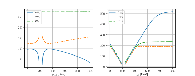
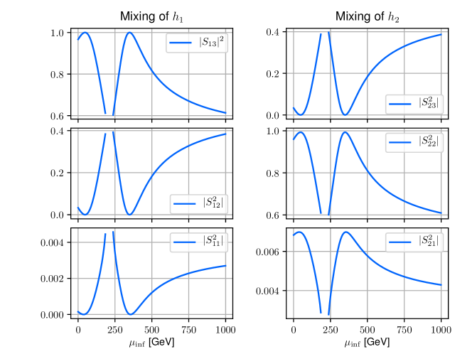
Figure 1: The masses of scalar higgses $h_{1}$, $h_{2}$, pseudoscalar higgs $a$, neutralinos ${\tilde{\chi}}^{0}_{1}$, ${\tilde{\chi}}^{0}_{2}$, and chargino ${\tilde{\chi}}^{\pm}_{1}$, depending on $\mu_{\text{inf}}$.

 

Figure 2: The three mixing components of two lightest Higgs bosons depending on $\mu_{\text{inf}}$. From bottom to top: the down type components are $|S_{11}^{2}|$ and $|S_{21}|^{2}$, the up type components are $|S_{12}|^{2}$ and $|S_{22}|^{2}$, and the singlet components are $|S_{13}|^{2}$ and $|S_{23}|^{2}$.

 

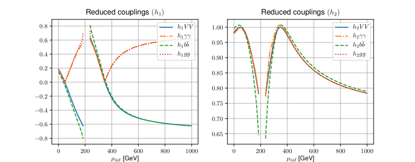
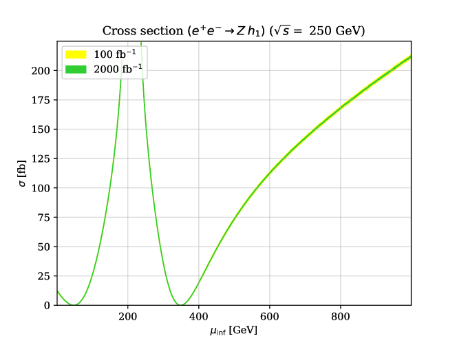
Figure 3: The reduced couplings of $h_{1}$ and $h_{2}$ to gauge bosons, photons, $b$ quarks and gluons, depending on $\mu_{\text{inf}}$.

 

Figure 4: The lightest scalar Higgs production cross section at 250 GeV ILC depending on $\mu_{\text{inf}}$.

 

Crucial for the phenomenology of this scenario is a view on the Higgs mixing matrices, especially the singlet-doublet mixings as shown in Fig. 2. Here, we show the singlet admixture to the lightest state (left side top), and the doublet components of the same (left side middle and down). On the right hand side, the same is shown for the second lightest state. It is interesting to see that there are two degenerate points, where $h_{1}$ is purely singlet and $h_{2}$ purely doublet. These points coincide with the minima and maxima in the spectrum of Fig. 2. Towards large values of $\mu_{\text{inf}}$, the second lightest Higgs becomes singlet-dominated, while the lightest loses its singlet character. Note, however, that there is no scalar at $125\,\textrm{GeV}$ in the spectrum anymore, so the regime of large $\mu_{\text{inf}}$ is disfavoured by observations.

The Higgs mixing also defines the reduced couplings at the tree level, see Eqs. (11) and (12). The reduced couplings as delivered by NMSSMTools are shown in Fig. 4, where we display the reduced couplings to electroweak gauge bosons ($VV$), photons ($\gamma\gamma$), bottom quarks ($b\bar{b}$), and gluons ($gg$) for the lightest and second lightest Higgs, $h_{1}$ and $h_{2}$ respectively. It can be seen that for the two points mentioned above with $\mu_{\text{inf}}\simeq 46\,\textrm{GeV}$ and $\simeq 348\,\textrm{GeV}$ the reduced couplings of $h_{2}$ approach the SM values, where in contrast the couplings of $h_{1}$ turn to zero. This is exactly the pure singlet case. In the neighbouring regime, the singlet-like state has small couplings to the SM and the couplings of $h_{2}$ deviate from the SM values. It is furthermore interesting to notice that the reduced couplings of the lightest state $h_{1}$ to gauge bosons and bottom quarks have the same absolute value but opposite signs in the regime $46\,\textrm{GeV}\lesssim\mu_{\text{inf}}\lesssim 348\,\textrm{GeV}$. This gives a handle to distinguish finally the two degenerate spectra for different values of $\mu_{\text{inf}}$. Especially for the point degenerate with the NMSSM case as discussed above for $\mu_{\text{inf}}=395\,\textrm{GeV}$, the reduced couplings to $b$ quarks and vector bosons have the opposite sign while the whole spectrum is identical. This reduced couplings can be, to some extend, identified with the coupling modifiers in the $\kappa$ framework for SM Higgs studies, as pointed out in Sec. 2.1. This becomes more relevant in the following section, where we study a scenario with a very SM-like Higgs over the full $\mu_{\text{inf}}$ range.

The couplings to gauge bosons, especially the $Z$ boson, also define the behaviour of the production cross section at a lepton collider, such as the ILC, in the dominant production mode via Higgsstrahlung. We display in Fig. 4 how the cross section for $e^{+}e^{-}\to Z\,h_{1}$ evolves with $\mu_{\text{inf}}$ in this scenario for an initial center of mass energy $\sqrt{s}=250\,\textrm{GeV}$. Of course, the pure singlet case at $\mu_{\text{inf}}=48\,\textrm{GeV}$ and $348\,\textrm{GeV}$ cannot be produced. With a certain doublet admixture, however, a light singlet-like state can be produced at the ILC250 with a few femtobarn cross section. The coloured bands show the statistical uncertainties for integrated luminosities of $L=100/\mathrm{fb}$ (yellow) and $L=2000/\mathrm{fb}$ (green). The cross section uncertainty is derived as statistical uncertainty from a counting analysis:

$$\delta\sigma=\frac{\sigma}{\sqrt{N}}=\sqrt{\frac{\sigma}{L}},$$ (20)

where the Poisson distribution defines the uncertainty from the number of signal events as $\sqrt{N}$. A delicate analysis of the discovery potential is beyond the scope of this paper. The simplified procedure described above for an estimate relies on a theoretical prediction under the assumption of a perfect experiment and thus neglecting detector effects.

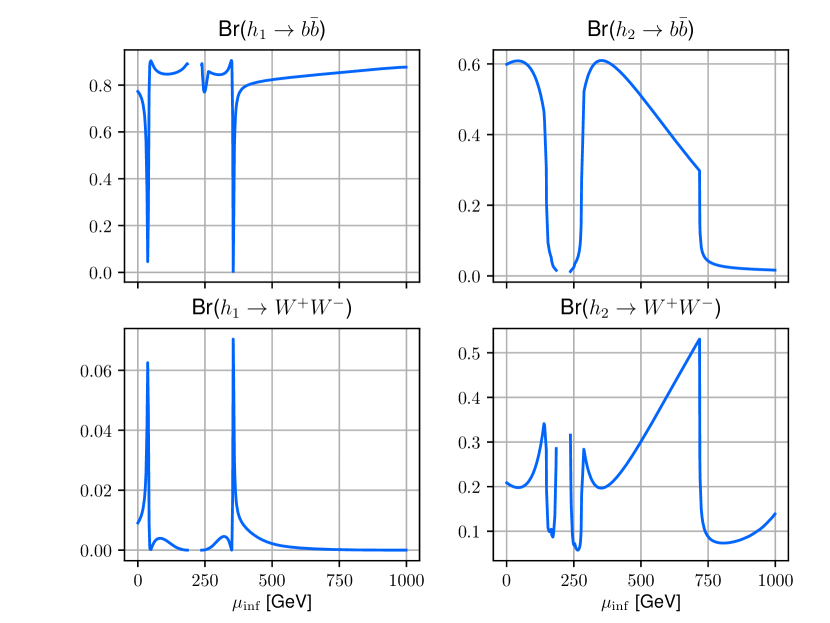
Figure 5: The branching ratios of $h_{1}$ and $h_{2}$ decay to $b$ quarks or $W$ bosons depending on $\mu_{\text{inf}}$.

 

Finally, we show the branching ratios for decays to bottom quarks and $W$ boson pairs in Fig. 5. The light state $h_{1}$ mainly decays to bottom quarks over most of the displayed $\mu_{\text{inf}}$ range. Only at the points where it becomes exclusively singlet, the branching ratio to bottom quarks drops towards zero. For the second lightest state, the branching ratio to bottom quarks also goes down in the interval $125\,\textrm{GeV}\lesssim\mu_{\text{inf}}\lesssim 275\,\textrm{GeV}$, which is partially compensated by an increase in decays to $W$ bosons. For a more detailed study of the behaviour, all decay modes have to be included. The rapid decrease of branching fractions of $h_{2}$ into both $b\bar{b}$ and $W$ pairs at below $\mu_{\text{inf}}\simeq 750\,\textrm{GeV}$ is due to the opening of the $h_{2}\to h_{1}h_{1}$ decay channel, where $m_{h_{2}}$ becomes twice $m_{h_{1}}$. The displayed branching ratios of $h_{2}$ go down in the window around $\mu_{\text{inf}}\simeq 200\,\textrm{GeV}$ because here the decays into neutralinos and charginos become relevant (notice their corresponding small masses in this window). The two dips in $\operatorname{Br}(h_{2}\to W^{+}W^{-})$ are due to an enhanced $\operatorname{Br}(h_{2}\to{\tilde{\chi}}_{1}^{0}{\tilde{\chi}}_{2}^{0})$ in these regimes.

3.3 Reweighting $\mu_{\text{inf}}$ effects in the spectrum

It has been remarked in a previous study of the inflationary $\mu$NMSSM, Ref. [5], that the neutralino spectrum at the tree level stays invariant under changes of $\mu_{\text{inf}}$ when the singlet self-coupling $\kappa$ is adjusted appropriately. Under the same redefinition also the scalar spectrum does not change over vast regions in the parameter range aside from extreme configurations. Such an extreme case has been discussed in Ref. [5]. In the following, we refrain from artificial cancellations in the mass matrices and choose rather combinations of parameters to be constant such that variations in $\mu_{\text{inf}}$ enter mildly. From a quick study of the scalar mass matrix given in Eqs. (5), we see that three combinations are dominantly controlling the matrix elements. One is the sum $\mu_{\text{eff}}+\mu_{\text{inf}}$, then we have $\frac{\kappa}{\lambda}\mu_{\text{eff}}$ repeatedly appearing and furthermore the combination that has been replaced by the charged Higgs mass dominating the heavy doublet mass eigenvalue.

We treat the following combinations constant under variation of $\mu_{\text{inf}}$, which implies a redefinition of $\kappa$ and $\mu_{\text{eff}}$:

$$a= \;\mu_{\text{inf}}+\mu_{\text{eff}}\,,$$ (21a)

$$b= \;\frac{\kappa}{\lambda}\mu_{\text{eff}}\,,$$ (21b)

$$c= \;\mu_{\text{eff}}(\frac{\kappa}{\lambda}\mu_{\text{eff}}+A_{\lambda})\equiv\frac{1}{2}(m_{H^{\pm}}^{2}-m_{W}^{2}+v^{2}\lambda^{2})\sin 2\beta\,.$$ (21c)

Keeping these combinations fixed, under variation of $\mu_{\text{inf}}$ the upper left blocks of the Higgs mass matrices are unchanged. The other mass matrix elements with a residual $\mu_{\text{inf}}$ dependence can then be expressed as

$$M_{S,33}^{2}= \;\lambda^{2}v^{2}\left(\frac{\cos\beta\sin\beta}{a-\mu_{\text{inf}}}(\frac{c}{a-\mu_{\text{inf}}}-b)-\frac{\mu_{\text{inf}}}{a-\mu_{\text{inf}}}\right)+b(A_{\kappa}+4b)\,,$$ (22a)

$$M_{S,13}^{2}= \;M_{S,31}^{2}=\;v\lambda\left(2a\cos\beta-(\frac{c}{a-\mu_{\text{inf}}}+b)\sin\beta\right)\,,$$ (22b)

$$M_{S,23}^{2}= \;M_{S,32}^{2}=\;v\lambda\left(2a\sin\beta-(\frac{c}{a-\mu_{\text{inf}}}+b)\cos\beta\right)\;,$$ (22c)

and

$$M_{P,33}^{2}= \;\lambda^{2}v^{2}\left(\frac{\cos\beta\sin\beta}{a-\mu_{\text{inf}}}(3b+\frac{c}{a-\mu_{\text{inf}}})-\frac{\mu_{\text{inf}}}{a-\mu_{\text{inf}}}\right)\;,$$ (23a)

$$M_{P,13}^{2}= \;M_{P,31}^{2}=\;-v\lambda\left(3b-\frac{c}{a-\mu_{\text{inf}}}\right)\sin\beta\;,$$ (23b)

$$M_{P,23}^{2}= \;M_{P,32}^{2}=\;-v\lambda\left(3b-\frac{c}{a-\mu_{\text{inf}}}\right)\cos\beta\;.$$ (23c)

Note, that the parameters $\lambda$, $A_{\kappa}$, and $\tan\beta$ can be essentially varied without changing the fixed combinations from above. Since we are studying the pure effect of $\mu_{\text{inf}}$ while minimally invasively changing the mass spectrum, we also keep them at the values specified in Tab. 3, where $\kappa$ is not kept at that value. This can be seen also from Eqs. (22) and (23) where the appearance of $\kappa$ is absorbed. The mass spectrum is then only slightly changing under increase of $\mu_{\text{inf}}$ from $0\,\textrm{GeV}$ to $1000\,\textrm{GeV}$ in contrast to what has been shown in Sec. 3.2. We show the correspondance of Fig. 2 in Fig. 6.

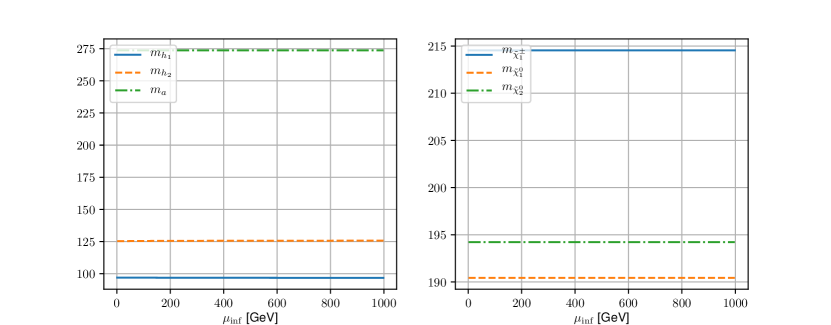
Figure 6: The masses of the light $\mathcal{CP}$-even states $h_{1}$, $h_{2}$, and the $\mathcal{CP}$-odd singlet-like state $a$ (left); the masses of the light neutralinos ${\tilde{\chi}}^{0}_{1}$, ${\tilde{\chi}}^{0}_{2}$, and the light chargino ${\tilde{\chi}}^{\pm}_{1}$ (right), depending on the pure $\mu_{\text{inf}}$ effect.

 

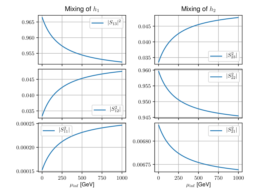
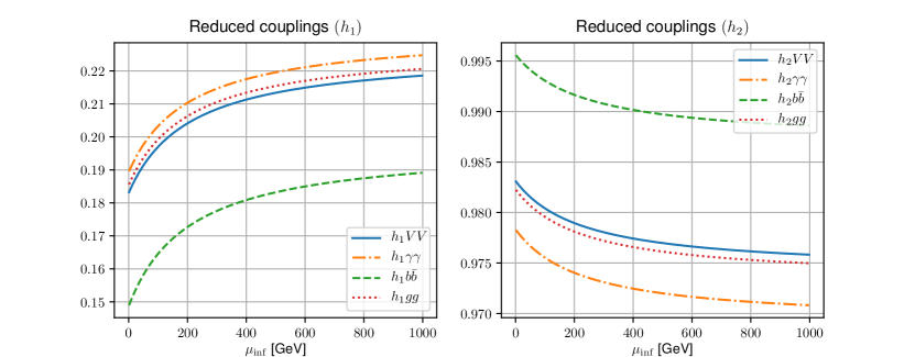
Figure 7: The three mixing components of the lightest scalar Higgses $h_{1,2}$ depending on the pure $\mu_{\text{inf}}$ effect. The down type component of $h_{1}$ is $|S_{11}^{2}|$, the up type component of $h_{1}$ is $|S_{12}^{2}|$ and the singlet component of $h_{1}$ is $|S_{13}^{2}|$.

 

Figure 8: The reduced couplings of $h_{1}$ and $h_{2}$ to gauge bosons, photons, $b$ quarks and gluons, depending on the pure $\mu_{\text{inf}}$ effect.

 

The question is now, how much the phenomenology of a $\mu$NMSSM point with large $\mu_{\text{inf}}$ differs from a point close to the NMSSM limit. Taking a look at the Higgs mixing components in Fig. 8, we see that the singlet admixture to the lightest state only mildly decreases. All changes in the mixings are less than at most $15\,\%$. It is interesting to notice that for increasing $\mu_{\text{inf}}$, the doublet admixture to the lightest Higgs increases, where simultaneously the doublet components in $h_{2}$ become less relevant. Moreover, the larger $\mu_{\text{inf}}$ the less rapid the change.

The behaviour of the mixing components with respect to $\mu_{\text{inf}}$ is also mirrored in the reduced couplings shown in Fig. 8. Measuring a deviation of less than $2\,\%$ from the SM-values for the SM-like scalar is more than challenging at the LHC and any future collider. Increasing $\mu_{\text{inf}}$ to around $1\,\textrm{TeV}$, we would have a deviation of less than $3\,\%$ for the coupling to photons, where the bottom quark coupling of $h_{2}$ deviates only a bit more than $1\,\%$ from the SM. Since for larger $\mu_{\text{inf}}$ the curves flatten out, a further increase of $\mu_{\text{inf}}$ in this scenario does not give a sizeable effect. On the other hand, the singlet-like scalar $h_{1}$ shows couplings of around $15-20\,\%$ of a SM-Higgs at the same mass of $97\,\textrm{GeV}$. That means, if non-vanishing couplings can be measured to more than $10\,\%$ at a future collider, there is a clear discovery potential for this singlet-like state. Nevertheless, it looks less promising to distinguish the $\mu$NMSSM-scenario from the NMSSM point by just comparing the reduced couplings in the $\kappa$ framework. If we look e. g. on the $h_{2}$ coupling to vector bosons in Fig. 8 (the blue continuous curve), which can be identified with $\kappa_{V}$, there is a variation of less than $0.01$ over the displayed range. Supposed that at the ILC this $\kappa_{V}$ can be measured to more than $1\,\%$ accuracy [56], a deviation might be visible. The corresponding measurements of the signal strength for the singlet-like state, however, look more promising.

The same effect can also be seen in the total widths of $h_{1}$ and $h_{2}$ displayed in Fig. 10, where the curves follow the behaviour of the reduced couplings. Due to the rather small total width of the lightest Higgs boson, the effect of an increasing $\mu_{\text{inf}}$ is very prominent here, where the total width is nearly doubled over the displayed range. In contrast, for $h_{2}$ the total width is only mildly affected and its variation probably out of reach. Since we are on top of the SM-value for the total width around $4\,\textrm{MeV}$, see Refs. [57, 27], there is also not much room for invisible decay modes that are also not predicted in this scenario.

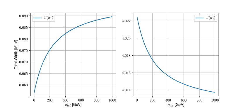
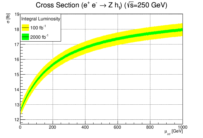
Figure 9: The total widths of the lightest scalar Higgs $h_{1}$ and second lightest Higgs $h_{2}$ depending on the pure $\mu_{\text{inf}}$ effect.

 

Figure 10: The lightest scalar Higgs production cross section at 250 GeV ILC depending on the pure $\mu_{\text{inf}}$ effect.

 

For a future study of this model at a collider, especially an $e^{+}e^{-}$ machine, the production cross section of the singlet-dominated state is important. We calculate the cross section in Higgstrahlung at the ILC for a center of mass energy $\sqrt{s}=250\,\textrm{GeV}$ as in Sec. 3.2. The result over the range $\mu_{\text{inf}}\in[0,1000]\,\textrm{GeV}$ is shown in Fig. 10. Starting from the NMSSM benchmark point with $\mu_{\text{inf}}=0\,\textrm{GeV}$ and a cross section of about $12.6\,\mathrm{fb}$, the total cross section is enhanced by about $50\,\%$ at $\mu_{\text{inf}}=1000\,\textrm{GeV}$. Already for $\mu_{\text{inf}}=200\,\textrm{GeV}$ there is an increase of one quarter with respect to the initial cross section in the pure NMSSM scenario. In general, we want to stress that cross sections of more than $10\,\mathrm{fb}$ are well in reach for a linear collider [58, 59, 60]. A cross section enhanced by $50\,\%$ compared to the NMSSM case is a clear sign of a possible distinction. The yellow and green coloured bands in Fig. 10 show the statistical uncertainties after an integrated luminosity of $100/\mathrm{fb}$ and $2000/\mathrm{fb}$, respectively. The interpretation of these uncertainty bands is most useful when distinguishing two parameter points for different values $\mu_{\text{inf}}$. At e. g. $\mu_{\text{inf}}=200\,\textrm{GeV}$ the uncertainty band allows for cross sections between $15.2$ and $16\,\mathrm{fb}$ with $100/\mathrm{fb}$ of recorded data. Similarly, a cross section of $16\,\mathrm{fb}$ hints of a $\mu_{\text{inf}}$ in the range between $200$ and $300\,\textrm{GeV}$. Nevertheless, for small values of $\mu_{\text{inf}}$, the uncertainties are also smaller in absolute terms and a $\mu_{\text{inf}}$ of $50\,\textrm{GeV}$ can be clearly distinguished from the $\mu_{\text{inf}}=0\,\textrm{GeV}$ case. If we assume that the ILC can reach an integral luminosity of up to $2000/\mathrm{fb}$, the statistical uncertainty is narrowed down giving a much higher potential for distinction. In this case a measured cross section can be assigned to a smaller range of $\mu_{\text{inf}}$ and conversely larger values of $\mu_{\text{inf}}$ could be distinguished at the experiment. Note that we have considered the statistical error only for the displayed cross section, especially we did not consider the detection efficiency and possible backgrounds in the experimental study. However, we believe that the ILC at $250\,\textrm{GeV}$ has a clear potential to distinguish the $\mu$NMSSM from the NMSSM as well as certain scenarios within the same model and encourage further experimental studies including detector effects.

4 Conclusions

We have studied in detail the electroweak phenomenology of a supersymmetric model which incorporates inflation in the early universe. The model has the same particle content as the NMSSM and comprises an additional singlet superfield. In contrast to the NMSSM, the speciality of our model is an additional $\mu$-term like in the MSSM originating from the non-minimal coupling to gravity, leading to the so called $\mu$NMSSM. Our study is focused on properties of the Higgs sector with a special emphasis on a light singlet-like state at $97\,\textrm{GeV}$. We have presented two routes how to distinguish a parameter point in the $\mu$NMSSM—where $\mu_{\text{inf}}$ is the parameter relevant for inflation—from a corresponding parameter point in the NMSSM. The benchmark point in the NMSSM has been chosen from a random scan over NMSSM-specific parameters obeying all current experimental constraints.

For the numerical study, we have employed the public code collection NMSSMTools which serves as spectrum generator and calculates several observables. NMSSMTools does not provide the input options for the $\mu$NMSSM, so we had to redefine the parameters in an appropriate way adopting the code for our model. We have identified a benchmark scenario to study the phenomenological differences of the NMSSM and the $\mu$NMSSM. This benchmark scenario provides an allowed parameter point in the NMSSM, where we have checked against existing collider physics constraints by the use of HiggsBounds/HiggsSignals and CheckMATE. Starting from this valid point with $\mu_{\text{inf}}=0\,\textrm{GeV}$, we have studied the full effect of $\mu_{\text{inf}}\neq 0\,\textrm{GeV}$ to see how the spectrum and the mixing changes once this parameter is turned on. We have found a drastic influence on the mass spectrum, especially with one region where the lightest Higgs states turns to be tachyonic. Over the full range of $\mu_{\text{inf}}$ we have identified one more parameter point where the mass spectrum of Higgs bosons and neutralinos/charginos is degenerate with the NMSSM point. However, taking a look at the reduced couplings of the singlet-like state to electroweak gauge bosons and bottom quarks, we see a difference in the sign which may give a potential for discinction of the two models. Furthermore, we have calculated the production cross section of the lightest Higgs in Higgsstrahlung at the ILC with a center of mass energy $\sqrt{s}=250\,\textrm{GeV}$. For the relevant physical points it is around $10\,\mathrm{fb}$ and offers the possibility for a detailed study at the linear collider.

As a second route to study the “pure” $\mu_{\text{inf}}$ effect, we have reweighted other parameters to keep the mass spectrum invariant under variations of $\mu_{\text{inf}}$. Even in this case, there is a sizeable effect on the Higgs mixing of a few percent and a reduction of the reduced couplings of the SM-like Higgs state to SM particles. Although the reduced couplings (or coupling-strength modifiers $\kappa$) deviate only by a few percent from the SM-value, such small deviations will be measureable at the future linear collider. In contrast, the singlet-like $\mathcal{CP}$-even state at $97\,\textrm{GeV}$ receives enhanced contributions to the couplings to SM-particles due to an enhanced doublet admixture. Here, the change for increased $\mu_{\text{inf}}$ is more prominent with several percent. It is important to notice that the reduced couplings of the singlet-like state with respect to a SM-Higgs at $97\,\textrm{GeV}$ are about $20\,\%$ and therewith sufficiently large. The Higgsstrahlung cross section of the lightest Higgs at ILC250 is also increasing with increasing $\mu_{\text{inf}}$ reaching $18\,\mathrm{fb}$ in the scenario under scrutiny. This offers the possibility to distinguish the NMSSM and $\mu$NMSSM scenarios from a measurement of the production cross section with sufficient integral luminosity.

References

- [1] M. B. Einhorn and D. R. T. Jones, “Inflation with Non-minimal Gravitational Couplings in Supergravity”, JHEP 03 (2010) 026, arXiv:0912.2718 [hep-ph].
- [2] S. Ferrara, R. Kallosh, A. Linde, A. Marrani, and A. Van Proeyen, “Jordan Frame Supergravity and Inflation in NMSSM”, Phys. Rev. D82 (2010) 045003, arXiv:1004.0712 [hep-th].
- [3] S. Ferrara, R. Kallosh, A. Linde, A. Marrani, and A. Van Proeyen, “Superconformal Symmetry, NMSSM, and Inflation”, Phys. Rev. D83 (2011) 025008, arXiv:1008.2942 [hep-th].
- [4] H. M. Lee, “Chaotic inflation in Jordan frame supergravity”, JCAP 1008 (2010) 003, arXiv:1005.2735 [hep-ph].
- [5] W. G. Hollik, S. Liebler, G. Moortgat-Pick, S. Paßehr, and G. Weiglein, “Phenomenology of the inflation-inspired NMSSM at the electroweak scale”, Eur. Phys. J. C79 no. 1, (2019) 75, arXiv:1809.07371 [hep-ph].
- [6] OPAL, G. Abbiendi et al., “Decay mode independent searches for new scalar bosons with the OPAL detector at LEP”, Eur. Phys. J. C 27 (2003) 311–329, arXiv:hep-ex/0206022.
- [7] LEP Working Group for Higgs boson searches, ALEPH, DELPHI, L3, OPAL, R. Barate et al., “Search for the standard model Higgs boson at LEP”, Phys. Lett. B 565 (2003) 61–75, arXiv:hep-ex/0306033.
- [8] ALEPH, DELPHI, L3, OPAL, LEP Working Group for Higgs Boson Searches, S. Schael et al., “Search for neutral MSSM Higgs bosons at LEP”, Eur. Phys. J. C47 (2006) 547–587, arXiv:hep-ex/0602042 [hep-ex].
- [9] CMS, A. M. Sirunyan et al., “Search for a standard model-like Higgs boson in the mass range between 70 and 110 GeV in the diphoton final state in proton-proton collisions at 8 and 13 TeV”, Phys. Lett. B 793 (2019) 320–347, arXiv:1811.08459 [hep-ex].
- [10] CMS, A. M. Sirunyan et al., “Search for additional neutral MSSM Higgs bosons in the final state in proton-proton collisions at 13 TeV”, JHEP 09 (2018) 007, arXiv:1803.06553 [hep-ex].
- [11] ATLAS, The ATLAS collaboration, “Search for resonances in the 65 to 110 GeV diphoton invariant mass range using 80 fb-1 of collisions collected at TeV with the ATLAS detector”,.
- [12] R. Dermisek and J. F. Gunion, “A Comparison of Mixed-Higgs Scenarios In the NMSSM and the MSSM”, Phys. Rev. D 77 (2008) 015013, arXiv:0709.2269 [hep-ph].
- [13] G. Belanger, U. Ellwanger, J. F. Gunion, Y. Jiang, S. Kraml, and J. H. Schwarz, “Higgs Bosons at 98 and 125 GeV at LEP and the LHC”, JHEP 01 (2013) 069, arXiv:1210.1976 [hep-ph].
- [14] J. Cao, X. Guo, Y. He, P. Wu, and Y. Zhang, “Diphoton signal of the light Higgs boson in natural NMSSM”, Phys. Rev. D 95 no. 11, (2017) 116001, arXiv:1612.08522 [hep-ph].
- [15] F. Domingo, S. Heinemeyer, S. Paßehr, and G. Weiglein, “Decays of the neutral Higgs bosons into SM fermions and gauge bosons in the -violating NMSSM”, Eur. Phys. J. C 78 no. 11, (2018) 942, arXiv:1807.06322 [hep-ph].
- [16] T. Biekötter, S. Heinemeyer, and C. Muñoz, “Precise prediction for the Higgs-boson masses in the SSM”, Eur. Phys. J. C 78 no. 6, (2018) 504, arXiv:1712.07475 [hep-ph].
- [17] T. Biekötter, M. Chakraborti, and S. Heinemeyer, “A 96 GeV Higgs boson in the N2HDM”, Eur. Phys. J. C 80 no. 1, (2020) 2, arXiv:1903.11661 [hep-ph].
- [18] T. Biekötter, S. Heinemeyer, and C. Muñoz, “Precise prediction for the Higgs-Boson masses in the SSM with three right-handed neutrino superfields”, Eur. Phys. J. C 79 no. 8, (2019) 667, arXiv:1906.06173 [hep-ph].
- [19] J. Cao, X. Jia, Y. Yue, H. Zhou, and P. Zhu, “96 GeV diphoton excess in seesaw extensions of the natural NMSSM”, Phys. Rev. D 101 no. 5, (2020) 055008, arXiv:1908.07206 [hep-ph].
- [20] J. M. Cline and T. Toma, “Pseudo-Goldstone dark matter confronts cosmic ray and collider anomalies”, Phys. Rev. D 100 no. 3, (2019) 035023, arXiv:1906.02175 [hep-ph].
- [21] K. Choi, S. H. Im, K. S. Jeong, and C. B. Park, “Light Higgs bosons in the general NMSSM”, Eur. Phys. J. C 79 no. 11, (2019) 956, arXiv:1906.03389 [hep-ph].
- [22] F. Richard, “Indications for extra scalars at LHC? – BSM physics at future colliders”, arXiv:2001.04770 [hep-ex].
- [23] J. A. Aguilar-Saavedra and F. R. Joaquim, “Multiphoton signals of a (96 GeV?) stealth boson”, arXiv:2002.07697 [hep-ph].
- [24] T. Biekötter, M. Chakraborti, and S. Heinemeyer, “The ”96 GeV excess” at the LHC”, 3, 2020. arXiv:2003.05422 [hep-ph].
- [25] U. Ellwanger and M. Rodriguez-Vazquez, “Discovery Prospects of a Light Scalar in the NMSSM”, JHEP 02 (2016) 096, arXiv:1512.04281 [hep-ph].
- [26] U. Ellwanger, C. Hugonie, and A. M. Teixeira, “The Next-to-Minimal Supersymmetric Standard Model”, Phys. Rept. 496 (2010) 1–77, arXiv:0910.1785 [hep-ph].
- [27] LHC Higgs Cross Section Working Group, J. R. Andersen et al., “Handbook of LHC Higgs Cross Sections: 3. Higgs Properties”, arXiv:1307.1347 [hep-ph].
- [28] U. Ellwanger, J. F. Gunion, and C. Hugonie, “NMHDECAY: A Fortran code for the Higgs masses, couplings and decay widths in the NMSSM”, JHEP 02 (2005) 066, arXiv:hep-ph/0406215 [hep-ph].
- [29] U. Ellwanger and C. Hugonie, “NMSPEC: A Fortran code for the sparticle and Higgs masses in the NMSSM with GUT scale boundary conditions”, Comput. Phys. Commun. 177 (2007) 399–407, arXiv:hep-ph/0612134 [hep-ph].
- [30] D. Das, U. Ellwanger, and A. M. Teixeira, “NMSDECAY: A Fortran Code for Supersymmetric Particle Decays in the Next-to-Minimal Supersymmetric Standard Model”, Comput. Phys. Commun. 183 (2012) 774–779, arXiv:1106.5633 [hep-ph].
- [31] F. Domingo, “A New Tool for the study of the CP-violating NMSSM”, JHEP 06 (2015) 052, arXiv:1503.07087 [hep-ph].
- [32] See: https://www.lupm.in2p3.fr/users/nmssm/README.
- [33] U. Ellwanger and C. Hugonie, “NMHDECAY 2.0: An Updated program for sparticle masses, Higgs masses, couplings and decay widths in the NMSSM”, Comput. Phys. Commun. 175 (2006) 290–303, arXiv:hep-ph/0508022.
- [34] P. Bechtle, O. Brein, S. Heinemeyer, G. Weiglein, and K. E. Williams, “HiggsBounds: Confronting Arbitrary Higgs Sectors with Exclusion Bounds from LEP and the Tevatron”, Comput. Phys. Commun. 181 (2010) 138–167, arXiv:0811.4169 [hep-ph].
- [35] P. Bechtle, O. Brein, S. Heinemeyer, O. Stål, T. Stefaniak, G. Weiglein, and K. E. Williams, “: Improved Tests of Extended Higgs Sectors against Exclusion Bounds from LEP, the Tevatron and the LHC”, Eur. Phys. J. C74 no. 3, (2014) 2693, arXiv:1311.0055 [hep-ph].
- [36] P. Bechtle, S. Heinemeyer, O. Stål, T. Stefaniak, and G. Weiglein, “: Confronting arbitrary Higgs sectors with measurements at the Tevatron and the LHC”, Eur. Phys. J. C 74 no. 2, (2014) 2711, arXiv:1305.1933 [hep-ph].
- [37] O. Stål and T. Stefaniak, “Constraining extended Higgs sectors with HiggsSignals”, PoS EPS-HEP2013 (2013) 314, arXiv:1310.4039 [hep-ph].
- [38] DELPHES 3, J. de Favereau, C. Delaere, P. Demin, A. Giammanco, V. Lemaître, A. Mertens, and M. Selvaggi, “DELPHES 3, A modular framework for fast simulation of a generic collider experiment”, JHEP 02 (2014) 057, arXiv:1307.6346 [hep-ex].
- [39] M. Cacciari, G. P. Salam, and G. Soyez, “FastJet User Manual”, Eur. Phys. J. C 72 (2012) 1896, arXiv:1111.6097 [hep-ph].
- [40] M. Cacciari and G. P. Salam, “Dispelling the myth for the jet-finder”, Phys. Lett. B 641 (2006) 57–61, arXiv:hep-ph/0512210.
- [41] M. Cacciari, G. P. Salam, and G. Soyez, “The anti- jet clustering algorithm”, JHEP 04 (2008) 063, arXiv:0802.1189 [hep-ph].
- [42] A. L. Read, “Presentation of search results: The CL(s) technique”, J. Phys. G 28 (2002) 2693–2704.
- [43] M. Drees, H. Dreiner, D. Schmeier, J. Tattersall, and J. S. Kim, “CheckMATE: Confronting your Favourite New Physics Model with LHC Data”, Comput. Phys. Commun. 187 (2015) 227–265, arXiv:1312.2591 [hep-ph].
- [44] D. Dercks, N. Desai, J. S. Kim, K. Rolbiecki, J. Tattersall, and T. Weber, “CheckMATE 2: From the model to the limit”, Comput. Phys. Commun. 221 (2017) 383–418, arXiv:1611.09856 [hep-ph].
- [45] S. Kraml, S. Kulkarni, U. Laa, A. Lessa, W. Magerl, D. Proschofsky-Spindler, and W. Waltenberger, “SModelS: a tool for interpreting simplified-model results from the LHC and its application to supersymmetry”, Eur. Phys. J. C 74 (2014) 2868, arXiv:1312.4175 [hep-ph].
- [46] C. K. Khosa, S. Kraml, A. Lessa, P. Neuhuber, and W. Waltenberger, “SModelS database update v1.2.3”, LHEP 158 (5, 2020) 2020, arXiv:2005.00555 [hep-ph].
- [47] P. Z. Skands et al., “SUSY Les Houches accord: Interfacing SUSY spectrum calculators, decay packages, and event generators”, JHEP 07 (2004) 036, arXiv:hep-ph/0311123.
- [48] B. Allanach et al., “SUSY Les Houches Accord 2”, Comput. Phys. Commun. 180 (2009) 8–25, arXiv:0801.0045 [hep-ph].
- [49] M. Muhlleitner, A. Djouadi, and Y. Mambrini, “SDECAY: A Fortran code for the decays of the supersymmetric particles in the MSSM”, Comput. Phys. Commun. 168 (2005) 46–70, arXiv:hep-ph/0311167.
- [50] Particle Data Group, P. Zyla et al., “Review of Particle Physics”, PTEP 2020 no. 8, (2020) 083C01.
- [51] G. Belanger, F. Boudjema, A. Pukhov, and A. Semenov, “MicrOMEGAs: A Program for calculating the relic density in the MSSM”, Comput. Phys. Commun. 149 (2002) 103–120, arXiv:hep-ph/0112278.
- [52] G. Belanger, F. Boudjema, C. Hugonie, A. Pukhov, and A. Semenov, “Relic density of dark matter in the NMSSM”, JCAP 09 (2005) 001, arXiv:hep-ph/0505142.
- [53] G. Belanger, F. Boudjema, A. Pukhov, and A. Semenov, “MicrOMEGAs 2.0: A Program to calculate the relic density of dark matter in a generic model”, Comput. Phys. Commun. 176 (2007) 367–382, arXiv:hep-ph/0607059.
- [54] G. Belanger, F. Boudjema, A. Pukhov, and A. Semenov, “micrOMEGAs_3: A program for calculating dark matter observables”, Comput. Phys. Commun. 185 (2014) 960–985, arXiv:1305.0237 [hep-ph].
- [55] G. Bélanger, F. Boudjema, A. Goudelis, A. Pukhov, and B. Zaldivar, “micrOMEGAs5.0 : Freeze-in”, Comput. Phys. Commun. 231 (2018) 173–186, arXiv:1801.03509 [hep-ph].
- [56] H. Bahl et al. BONN-TH 2019-04, DESY 19-093, KA-TP-09-2019, IFT-UAM/CSIC-19-075, to be published, private communication with S. Heinemeyer.
- [57] LHC Higgs Cross Section Working Group, D. de Florian et al., “Handbook of LHC Higgs Cross Sections: 4. Deciphering the Nature of the Higgs Sector”, arXiv:1610.07922 [hep-ph].
- [58] K. Fujii et al., “The Potential of the ILC for Discovering New Particles”, arXiv:1702.05333 [hep-ph].
- [59] A. Arbey et al., “Physics at the e+ e- Linear Collider”, Eur. Phys. J. C75 no. 8, (2015) 371, arXiv:1504.01726 [hep-ph].
- [60] H. Baer, T. Barklow, K. Fujii, Y. Gao, A. Hoang, S. Kanemura, J. List, H. E. Logan, A. Nomerotski, M. Perelstein, et al., “The International Linear Collider Technical Design Report - Volume 2: Physics”, arXiv:1306.6352 [hep-ph].