¹Courant Institute of Mathematical Sciences, New York University, New York, NY 10012
²Mathematical Biosciences Institute, The Ohio State University, Columbus, OH 43210
³Laboratoire Jacques-Louis Lions, Sorbonne Université, 75005 Paris, France
⁴Department of Mathematics and Statistics, Williams College, Williamstown, MA 01267
⁵Institute for the Quantitative Study of Inclusion, Diversity, and Equity, Williamstown, MA 01267
⁶Department of Computational Medicine, UCLA, Los Angeles, CA 90095
⁷Department of Mathematics, CSUN, Los Angeles, CA 91330
^∗C. Vallejo and J. Crodelle contributed equally to this work.
^†Corresponding author

April 28, 2020

Objectives: We examine crime patterns in Santa Monica, California before and after passage of Proposition 47, a 2014 initiative that reclassified some non-violent felonies to misdemeanors. We also study how the 2016 opening of four new light rail stations, and how more community-based policing starting in late 2018, impacted crime.
Methods: A series of statistical analyses are performed on reclassified (larceny, fraud, possession of narcotics, forgery, receiving/possessing stolen property) and non-reclassified crimes by probing publicly available databases from 2006 to 2019. We compare data before and after passage of Proposition 47, city-wide and within eight neighborhoods. Similar analyses are conducted within a 450 meter radius of the new transit stations.
Results: Reports of monthly reclassified crimes increased city-wide by approximately 15$\%$ after enactment of Proposition 47, with a significant drop observed in late 2018. Downtown exhibited the largest overall surge. The reported incidence of larceny intensified throughout the city. Two new train stations, including Downtown, reported significant crime increases in their vicinity after service began.
Conclusions: While the number of reported reclassified crimes increased after passage of Proposition 47, those not affected by the new law decreased or stayed constant, suggesting that Proposition 47 strongly impacted crime in Santa Monica. Reported crimes decreased in late 2018 concurrent with the adoption of new policing measures that enhanced outreach and patrolling. These findings may be relevant to law enforcement and policy-makers. Follow-up studies needed to confirm long-term trends may be affected by the COVID-19 pandemic that drastically changed societal conditions. Keywords: California Proposition 47 $\cdot$ Welch’s t-test $\cdot$ change-point analysis $\cdot$ segmented regression $\cdot$ light rail $\cdot$ community policing

1 Introduction and background

On November 4, 2014, voters of the state of California passed Proposition 47 (hereafter Prop. 47), also known as the “Criminal Sentences. Misdemeanor Penalties. Initiative Statute.” or “The Safe Neighborhoods and Schools” Act. The referendum, which was approved with 59.6$\%$ of the vote, went into effect the following day, November 5, 2014 (Ballotpedia, 2014). Prop. 47 imparted three broad changes to felony sentencing laws in the state of California: i) certain non-violent theft and drug possession offenses would be reclassified from felonies to misdemeanors; ii) those serving sentences for the reclassified offenses would be allowed to petition courts for re-sentencing; iii) those who had completed felony sentences now classified as misdemeanors would be able to petition courts to amend their criminal records. Felonies reclassified as misdemeanors under Prop. 47 include shoplifting, attempted shoplifting, grand theft auto, receiving stolen property, forgery, fraud, writing bad checks; each up to a maximum monetary value of 950 USD. Possession of most illegal drugs for personal use, including methamphetamine, heroin and cocaine, was also reclassified as a misdemeanor. The law allows for some exceptions, for instance reclassification may not apply if perpetrators have a criminal record including violence or sexual offenses.

Prop. 47 was part of a series of initiatives designed to lessen California’s incarcerated population in response to allegations of inadequate inmate medical and mental health care, amounting to cruel and unusual punishment. In 2009, federal courts required the state to reduce prison overcrowding and set an occupancy threshold of 137.5$\%$ of design capacity to guarantee inmates’ Eighth Amendment rights. On May 23, 2011 and upon appeal by the State of California, the US Supreme Court upheld this decision in Brown vs. Plata: California’s prison population would have to decrease from approximately 156,000 to 110,000 individuals (Newman and Scott, 2012). To comply with federal orders, state lawmakers enacted significant legislative reforms over the years, including Prop. 47. Assembly Bill (AB) 109, also known as the Public Safety Realignment Bill, and Assembly Bill 117, also known as the Criminal Justice Realignment Bill, were approved and went into effect on October 1, 2011 (Owen and Mobley, 2012). These laws allowed those convicted of certain non-violent crimes to serve their sentences in county facilities, under house arrest, or in alternative sentencing schemes, rather than in state prisons. Overall, 500 criminal statutes were amended and penalties for parole violations were reduced. On November 6, 2012, voters also approved Prop. 36, which revised California’s 1994 Three Strikes Law mandating a sentence of 25 years to life for those convicted of a third felony. Under Prop. 36, to be considered a strike, the third offense must be a serious or violent felony, or the perpetrator must have been previously convicted of murder, rape, or child molestation.

Although the state prison population fell after enactment of AB 109 and AB 117, it was only after passage of Prop. 47 that the incarcerated population dropped below the 2009 court-mandated target (Romano, 2015; Grattet and Bird, 2018; Mooney et al., 2019). One study found a 50$\%$ decline in the number of individuals being held or serving sentences for the reclassified crimes (Bird et al., 2016). Prop. 47 also stipulated that any resulting monetary savings should be diverted to crime prevention programs targeting youth and recidivists. The Safe Neighborhoods and Schools Fund was specifically created to manage these savings, estimated to be between 150 and 250 million USD per year. To date, $65\%$ of payments have been distributed to the Board of State and Community Correction, with the Department of Education and the Victim Compensation and Government Claims Board receiving minor percentages (Taylor, 2016). Reducing penalties for drug possession may have also lessened racial and ethnic disparities in the California criminal justice system (Mooney et al., 2018).

While Prop. 47 helped reduce incarceration, determining its effects on the reclassified crime rates has proven more controversial. Several parties, including law enforcement officials, district attorneys, and mayors point to the law for rising crime (Lehner, 2016; Casuso, 2018; Egelko, 2018; Weisberg, 2019). Some studies link moderate (Bartos and Kubrin, 2018) or sustained (Bird et al., 2018; Fischer, 2018) crime increases to the enactment of Prop. 47, while other groups maintain that current data is inconclusive and that a longer term perspective is necessary (Males, 2016). Aside from the disputed effects of Prop. 47 on crime rates, it has also been claimed that the new law brought unintended consequences such as the elimination of DNA collection for the reclassified crimes, restrictions in arresting repeat offenders, declines in the reporting of crimes as victims learned that police would not be able to apprehend and punish perpetrators, and making habitual drug users less likely to seek treatment (Hanisee, 2018). A preliminary analysis conducted state-wide by the California Police Chiefs Association finds that the consequences of Prop. 47 are not homogeneous among cities of comparable size and that county specific factors, such as efficacy of monitoring and treatment programs, and how probation and/or incarceration are handled locally, may affect crime rates (Lehner, 2016). Judging the outcomes of Prop. 47 has led to a contentious debate within academic, political, and community settings, culminating in a growing movement to reverse some of its reforms through a proposed 2020 ballot initiative (Keep California Safe, 2020). Public safety agencies, caught between opposite viewpoints on the overall positive or negative societal effects of Prop. 47, have often expressed the need to better understand its consequences to optimize operations and budgets, to improve procedures, and to share impartial findings with stakeholder groups (Hunter et al., 2017).

The goal of this work is to investigate the impacts of Prop. 47 on crime rates in the coastal city of Santa Monica, California, population 91,411 (2019). Located in Los Angeles County, the city is bordered by Los Angeles proper and the Pacific Ocean. Its downtown core has recently undergone intense revitalization, fueled by high-tech start-ups, increased tourism, and the 2016 opening of the Metro Expo Line light rail extension. The latter now connects the beach with nearby Culver City and inner Los Angeles neighborhoods through seven new stations of which four are located within municipal borders. The city has also experienced rising housing costs, the displacement of long-term tenants, and increasing levels of homelessness (Kamel, 2012; Holland and Smith, 2017). In recent years both the Santa Monica Police Department (SMPD) and the local press have reported increases in crime, including robbery, burglary, aggravated assault, and homicide, with large numbers of repeat offenders (Sheriff’s Department, 2018; Cagle, 2018; Catanzaro, 2019; Pauker, 2019c ). Dedicated social media accounts and resident neighborhood groups (Residocracy Santa Monica, 2020; Santa Monica Now, 2020; Santa Monica Crime Watch, 2020; Santa Monica Problems, 2020) have been awash with images, anecdotal evidence and speculations on the root cause of these trends. Passage of Prop. 47 is among the theories offered to explain the rise in crime; another is the opening of the Expo Line allowing for easier transportation to and from the city (Cervantes, 2016; Neworth, 2017; Harlander, 2018). After a change in leadership in May 2018, the SMPD launched a series of new public safety initiatives. These included hiring twenty new police officers, increasing patrolling and outreach efforts, establishing a dedicated unit to analyze crime trends, deploying nightly security guards, adding lighting and CCTV cameras to public garages, and even limiting the hours of operations of some businesses that attracted large amounts of crime Renaud, (2019). The SMPD also increased its engagement with people experiencing homelessness and former inmates, helping them connect to services. Among the newly established programs are the Neighborhood Resource Officers to facilitate community-oriented policing, the Homeless Liaison Program, to assist the unhoused, and the Downtown Business Services Unit to improve communication with business owners. These initiatives are reported to have mitigated crime in the city, especially those affecting quality of life Pauker, 2019a ; Pauker, 2019b .

As part of its pledge towards greater transparency, the SMPD maintains a publicly-available crime database, listing dates, types, and locations of crimes within its jurisdiction starting from January 2006 until the present day (Santa Monica Police Department, 2020). Motivated by the many changes to the city, and to better quantify how violence and crime have changed over the past thirteen years, we performed several statistical analyses on this large body of data with a specific focus on identifying possible effects of Prop. 47. Our data analysis is meant as a first step in quantifying long-term crime trends in Santa Monica, and as a way to go beyond casual information and/or personal opinion. Throughout our work, in every instance where we discuss changes to crime trends it is important to note that any increase or decrease we present applies only to the reported crimes listed by the SMPD. This qualifier is crucial, as inferring true crime trends would require perfect knowledge, and the SMPD data may not be an unbiased representative sample of the actual crimes committed. For example, the data may be affected by biases in collection methods, changes to police routines, changes in the public’s habits, and more.

Given the above caveat, we find that the average number of reclassified monthly crimes increased overall by about 15$\%$ after enactment of Prop. 47. The sharp increase clearly emerges in the latter part of 2014, concurrent with passage and implementation of Prop. 47. A decrease in crime is observed towards the end of 2018 and persists through 2019, concurrent with the new police initiatives illustrated above. Longer term studies would be needed to determine whether this decrease will stabilize in the future. A geographical analysis reveals that overall the incidence of reclassified crimes after passage of Prop. 47 increases or stays constant in all but one of the eight Santa Monica neighborhoods, with significant rises in monthly counts in Downtown ($+37.2\%$) and the North of Montana and Ocean Park neighborhoods ($+13.2\%$ and $+12.0\%$, respectively). Non-reclassified crimes instead appear to decrease in all districts, except for Downtown which saw an $8.9\%$ increase.

Finally, we analyze monthly average crime rates within 450 meters of the four new Expo Line train stations opened in Santa Monica in May 2016. Of these, the Downtown Santa Monica and 17^th Street/Santa Monica College stops exhibit a statistically significant increase for all crimes after May 2016; the difference is not significant for the 26^th Street/Bergamot and Expo/Bundy stops. The first two stations are marked by a larger number of crime attractors and foot traffic than the other two. Crime percent increases are similar for both reclassified (+30.6$\%$) and non-reclassified (+34.6$\%$) crimes at Downtown Santa Monica. At 17^th Street/Santa Monica College instead the percent increase of reclassified crimes (+38.6$\%$) is much larger than that of non-reclassified crimes (+20.6$\%$). Finally, reclassified crimes increase at 26^th Street/Bergamot (+30.0$\%$) but non-reclassified ones do not vary appreciably. These results suggest that Prop. 47 led to differential crime increases at the Expo Line train stations.

Our conclusions stem from multiple statistical analyses performed on the data, which we present in Sect. 2. In Sect. 3.1, we use a Welch’s t-test to show that the average monthly number of crimes affected by Prop. 47 after November 2014 is significantly larger than prior to that date. We further decompose the full 2006-2019 crime time series into three components: a trend, a periodic seasonality, and a random residual, in Sect. 3.2. The resulting trend increases around the end of 2014, as discussed in Sects. 3.3 and 3.4, where change-point analysis and segmented regression analysis are used to determine trend change loci. In Sect. 4 and 5 we analyze crime trends in each of the eight neighborhoods that comprise the city of Santa Monica and the more circumscribed ones associated with the opening of the Expo Line. Finally, we present a discussion and conclusion illustrating limitations and possible extensions of this work in Sect. 6.

Understanding city-wide and neighborhood effects of Prop. 47 as well as how the opening of new train stations affect the geography of crime, may help administrators and law enforcement better plan intervention strategies, optimize resource allocation, and prioritize budget spending, especially in light of savings due to reduced incarceration.

2 Data

Prop. 47 crimes	Count
Larceny	37,082
Fraud	7,121
Narcotics possession	3,549
Forgery	1,458
Receiving/Possessing stolen property	636
Total	49,846
non-Prop. 47 crimes	Count
Assault	13,870
Public intoxication	12,926
Vandalism	9,699
Burglary	8,724
Grand theft auto (GTA)	4,812
Contempt of court	4,295
DUI	3,724
Robbery	2,317
Sex Offenses	1,128
Narcotic sale	456
Total	61,951
All Crimes	111,797

Table 1: Crimes considered in this work and their cumulative count between 2006 and 2019. The Prop. 47 (reclassified) crimes are those subject to reclassification; the non-Prop. 47 (non-reclassified) crimes are those not affected by legislative change.

The data used in this study was obtained from an open source file managed and updated by the Santa Monica Police Department (SMPD) from January 2006 to the present day (Santa Monica Police Department, 2020). The raw data includes the Uniform Crime Reporting (UCR) classification code as determined by the FBI (Federal Bureau of Investigation, 2004), a description of the type of crime, the date on which it occurred, and the latitude and longitude of its location. To better manage the information and perform statistical analyses on categories with a sufficient amount of data, we collapsed some original crime categories into coarser ones. For instance, we grouped “aggravated assault with a firearm,” “general aggravated assault,” “aggravated assault with hands,” “aggravated assault with knife,” and “aggravated assault with other weapon,” under the new general category “assault.” We also set a threshold of 450 counts per category, so that if this minimum number of crime occurrences was not met over the 2006-2019 period, the category was excluded from our analysis due to insufficient data. Among the crimes that did not meet the threshold were arson, embezzlement, blackmail and homicide. Misappropriation of property appears in the database only from 2010 onwards so we also discarded this category from our analysis. Finally, all incomplete or corrupted entries were discarded.

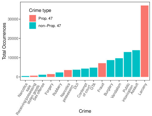
Figure 1: Visualization of the total number of crimes in Santa Monica from 2006 to 2019, as listed in Table 1. Receiving and possessing stolen goods, forgery, narcotics possession, fraud and larceny are all reclassified crimes. All others do not fall under the provisions of Prop. 47.

In Table 1 we list the general crime categories that were reclassified from felonies to misdemeanors under Prop. 47 and their respective 2006-2019 city-wide counts. They are larceny, fraud, narcotics possession, forgery, and receiving/possessing stolen property. We refer to these collectively as “Prop. 47 crimes” or “reclassified crimes.” Crimes not affected by Prop. 47 are also listed in Table 1 as “non-Prop. 47 crimes;” we will also refer to them as “non-reclassified crimes.” Note that their cumulative counts are of the same order of magnitude as the reclassified ones. The crime database is updated by the Santa Monica Police Department daily; for most of our analysis we consider monthly, or in some cases yearly, aggregates. In the following sections we compare temporal trends between the two groups of crimes to determine the effects of the 2014 initiative. Fig. 1 gives an overall view of the data. Larceny, one of the Prop. 47 offenses, has the highest overall incidence followed by assault and public intoxication, both non-Prop. 47 crimes. Fig. 2 displays the total (reclassified and non-reclassified) annual crime count from 2006 through 2019.

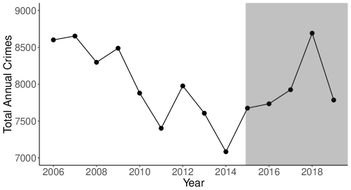
Figure 2: Total number of annual crimes from 2006 to 2019. The gray area indicates the years during which Prop. 47 was enforced. Note the lowest crime point in 2014, and the sharp decline in 2019.

Prop. 47 imposed a maximum monetary value of 950 USD for crimes to be reclassified as misdemeanors; however, no dollar amount information is specified in the data set we examined. We used ancillary information to determine which categories should fall under the Prop. 47 header, depending on their typical economic value. For example, the FBI’s UCR Program for 2017 estimates the average value of property lost due to larceny to be roughly 1,007 USD per offense (Federal Bureau of Investigation, 2017). In earlier years, the average value of losses due to larceny was lower, for example in 2006 it was 855 USD per offense, justifying its inclusion in the Prop. 47 reclassified list for all years. Larceny is here broadly defined as the unlawful taking of property such as motor vehicle parts and accessories or bicycles, shoplifting and pick-pocketing. Since the average street value of cocaine, heroin or methamphetamine doses for personal use is well below the 950 USD threshold, we also include possession of narcotics in the Prop. 47 reclassified list. The Federal Reserve estimates that for the year 2015 total fraud from bad checks, general-purpose transactions, and credit card accounts, resulted in 62 million single payments for a total of 8.3 billion USD, averaging 135 USD per transaction (Federal Reserve System, 2018). We thus include fraud and forgery in the Prop. 47 crime list. Finally, we do not include grand theft auto in the list of Prop. 47 crimes, since as per conversations with the SMPD, the typical value of stolen vehicles exceeds 950 USD, and thus grand theft auto incidents may fall outside the scope of Prop. 47. The SMPD also confirmed that the monetary value associated with all the Prop. 47 crimes listed in Table 1 is usually under the 950 USD threshold imposed for reclassification purposes.

We do not adjust crime counts for population change since the number of Santa Monica inhabitants has remained fairly stable in the thirteen year period under investigation. The city tallied approximately 87,000 residents in 2006, and after peaking at 93,000 in 2015, the population is currently estimated to be 91,411 (World Population Review, 2018).

3 Effects of passage of Proposition 47

We now perform a series of statistical analyses on the two data sets identified in Table 1: the Prop. 47 crimes (possession of narcotics, fraud, larceny, forgery, receiving and possessing stolen property), and the non-Prop. 47 crimes (all others not affected by legislative change). To illustrate the geographical variability of crime, Fig. 3 displays a map of the average annual incidence of larceny (a reclassified crime) before (2006-2014) and after (2015-2019) implementation of Prop. 47. Most events are located in downtown Santa Monica, with the average annual crime density increasing after 2014, as can be seen by the more intense coloring in the right-hand panel of Fig. 3.

3.1 The monthly mean number of reclassified crimes increases after implementation of Prop. 47

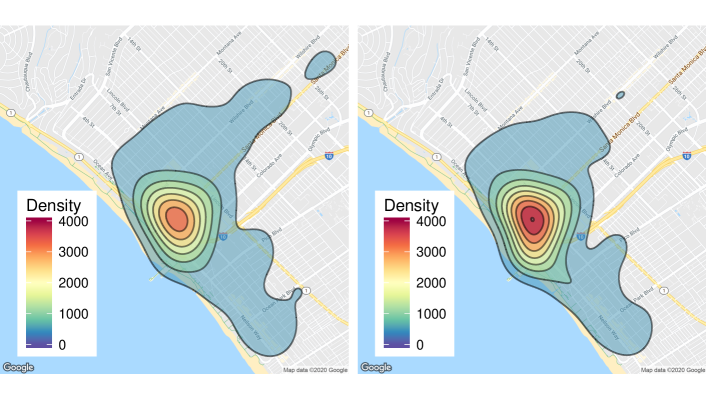
Figure 3: Contour map of annual larceny crimes before Prop. 47 (left) and after Prop. 47 (right). The right-hand panel displays more intense coloring in the central contours, reflecting higher incidence of larceny after implementation of Prop. 47. Although the specific visualization pertains to larceny, all crime types are more prevalent Downtown compared to residential areas.

To quantify the effects of Prop. 47 on crime rates in Santa Monica, we compute the average number of monthly offenses subject to reclassification before and after passage of Prop. 47. For comparison we perform the same analysis on the non-Prop. 47 crimes. Although the specific implementation of Prop. 47 occurred on November 5, 2014, we group all November 2014 events as occurring after passage of the new law since we are binning data by the month. Histograms for the four resulting subsets of data are shown in Fig. 4. The before and after monthly crime distributions for Prop. 47 offenses are presented in the left-hand panel of Fig. 4; before and after distributions for non-Prop. 47 crimes are in the right-hand panel of Fig. 4. As can be seen, the Prop. 47 crime distribution is shifted to the right after November 2014 with respect to the pre-implementation data. On the other hand, the post-November 2014, non-Prop. 47 crime distribution is shifted to the left. These histograms suggest that crimes affected by the reclassification process increased after passage of Prop. 47 whereas the incidence of crimes that were not subject to the new legislation decreased. To determine whether these shifts are statistically significant we use Welch’s unequal variances t-test (Welch’s t-test) to compare the before and after mean monthly count of reclassified crimes. This is a two-sample test typically employed to compare two mean values when the respective samples have unequal size or variance (Welch, 1947). In our specific case, data is available over eight years (106 months) before November 2014 and only over five years (62 months) after the same date, leading to very different sample sizes and variances. If the occurrence of Prop. 47 crimes listed in Table 1 were not affected by the reclassification process, we would expect the difference between crime counts before and after passage of the law as determined by Welch’s t-test to be negligible.

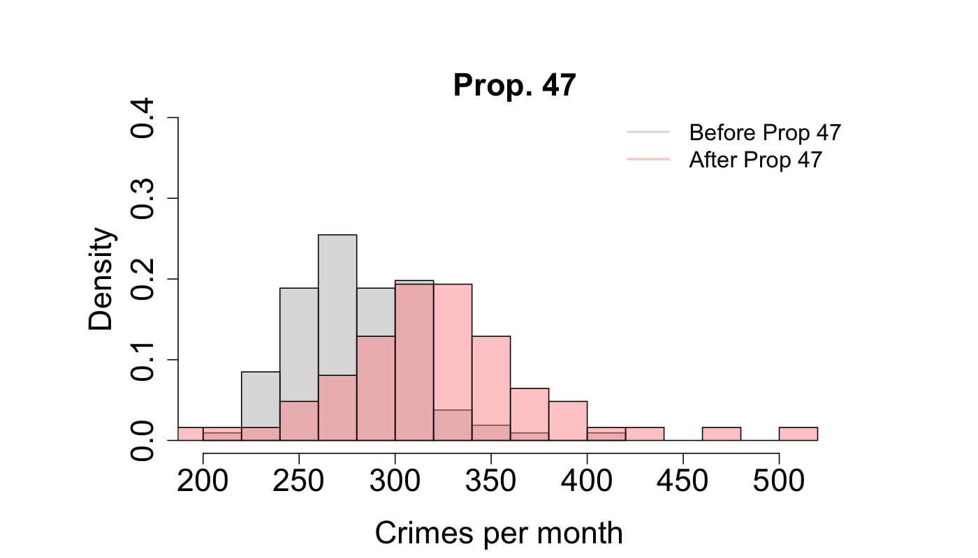
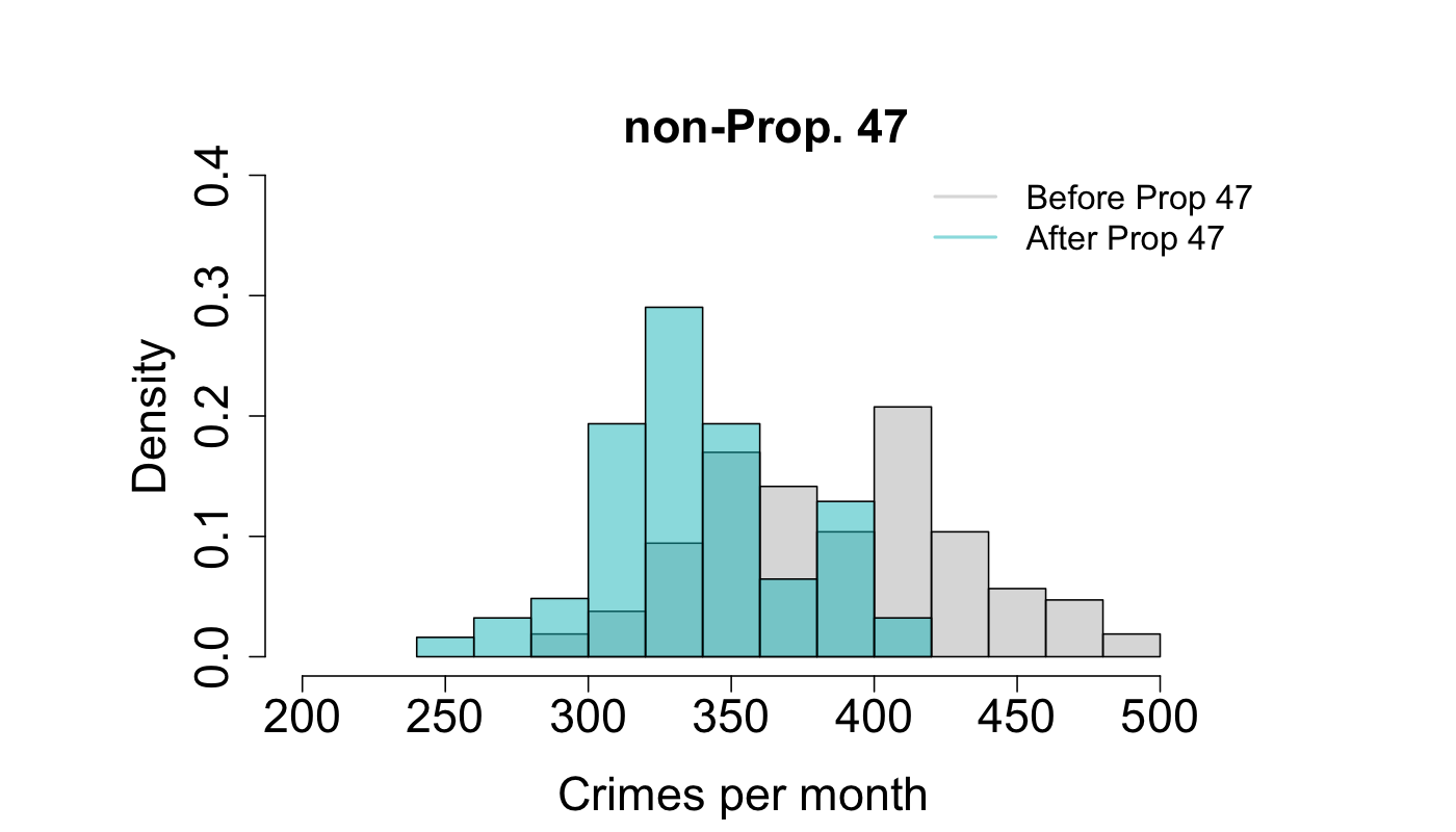
Figure 4: Histograms of crime counts per month before November 2014 for Prop. 47 crimes, subject to reclassification (left), and non-Prop. 47 crimes, not affected by legislative change (right). For Prop. 47 crimes, the monthly average before implementation of the new law was 281.4 crimes, whereas after November 2014 the average was 322.9 crimes per month. Performing a Welch’s t-test shows that this 14.7% increase in the average number of crimes per month is statistically significant at the 0.05 level. The same computations applied to non-Prop. 47 crimes show that, to the contrary, non-reclassified crimes decrease by 13%, from 387.3 to 337.1 per month, after passage of the initiative.

We denote by $\mu_{\text{b}}$ and $\mu_{\text{a}}$ the mean monthly number of Prop. 47 crimes before and after November 2014, respectively; $\sigma_{\text{b}}$ and $\sigma_{\text{a}}$ represent the associated standard deviations, and $N_{\text{b}}$ and $N_{\text{a}}$ the respective number of months over which these averages were calculated. The null hypothesis is formulated as there being no difference in the mean values, $\mu_{\text{b}}$ = $\mu_{\text{a}}$, while the alternative hypothesis posits that Prop. 47 led to an increase in the reclassified offenses, $\mu_{\text{b}}<\mu_{\text{a}}$. Our data yields $\{\mu_{\text{b}},\sigma_{\text{b}},N_{\text{b}}\}_{\rm p47}=\{281.4,33.2,106\}$ and $\{\mu_{\text{a}},\sigma_{\text{a}},N_{\text{a}}\}_{\rm p47}=\{322.9,53.9,62\}$. The ‘p47’ subscript indicates that these statistical values are evaluated on Prop. 47 offenses. To verify whether the before-to-after crime increase is statistically significant we perform a one-tailed Welch’s t-test by calculating the following $t$-statistic

$$t=\frac{\mu_{\rm{b}}-\mu_{\rm{a}}}{\displaystyle{\sqrt{\frac{\sigma^{2}_{\rm{b}}}{N_{\text{b}}}+\frac{\sigma^{2}_{\rm{a}}}{N_{\text{a}}}}}},$$ (1)

yielding $t=5.5$ for the values listed above. This quantity must be compared to the corresponding $t$-value from the Student’s $t$-distribution (Walck, 2007), once the number of degrees of freedom $\nu$ and the significance level are specified. We denote this reference $t$-value as $t_{\rm s}$. Since the before and after Prop. 47 samples are associated to different data sets, each with their own degrees of freedom, we use the Welch-Satterthwaite equation to derive an effective $\nu$ (Satterthwaite, 1946)

$$\nu=\frac{\left(\displaystyle{\frac{\sigma_{\text{b}}^{2}}{N_{\text{b}}}}+\frac{\sigma_{\text{a}}^{2}}{N_{\text{a}}}\right)^{2}}{\displaystyle{\frac{\sigma_{\text{b}}^{4}}{N_{\text{b}}^{2}(N_{\text{b}}-1)}+\frac{\sigma_{\text{a}}^{4}}{N_{\text{a}}^{2}(N_{\text{a}}-1)}}},$$ (2)

from which we obtain $\nu=89$. Finally, we specify a significance level of $0.05$ to find the reference value $t_{\rm s}=1.66$ from the Student’s $t$-distribution. Since this quantity is much smaller than the $t=5.5$ statistic found from Eq. (1), we reject the null hypothesis in favor of the alternative one: the $15\%$ increase in the average monthly number of reclassified crimes after the introduction of Prop. 47 is statistically significant.

We perform a similar analysis for the non-reclassified crimes, using $\{\mu_{\text{b}},\sigma_{\text{b}},N_{\text{b}}\}_{\rm{non\,p47}}=\{387.3,44.8,106\}$ and $\{\mu_{\text{a}},\sigma_{\text{a}},N_{\text{a}}\}_{\rm{non\,p47}}=\{337.1,34.8,62\}$, where the subscript ‘non p47’ refers to values being evaluated on non-reclassified crimes before and after passage of Prop. 47. We formulate the same null hypothesis as above, $\mu_{\text{b}}$ = $\mu_{\text{a}}$, with the alternative hypothesis set as there being a decrease in the mean monthly number of crimes after November 2014, $\mu_{\text{b}}>\mu_{\text{a}}$. The $t$-statistic obtained from Eq. (1) and the non-Prop. 47 values is $t=8.1$; Eq. (2) yields $\nu=153$, which results in $t_{\rm s}$ = 1.66 at the 0.05 significance level. Since $t_{\rm s}=1.66<t=8.1$, we reject the null hypothesis in favor of the alternative one: the $13\%$ decrease in the average monthly number of non-reclassified crimes after the introduction of Prop. 47 is statistically significant.

Thus far, our analysis suggests that the monthly occurrence of reclassified crimes increased after passage of Prop. 47, whereas crimes that were not affected by it, decreased.

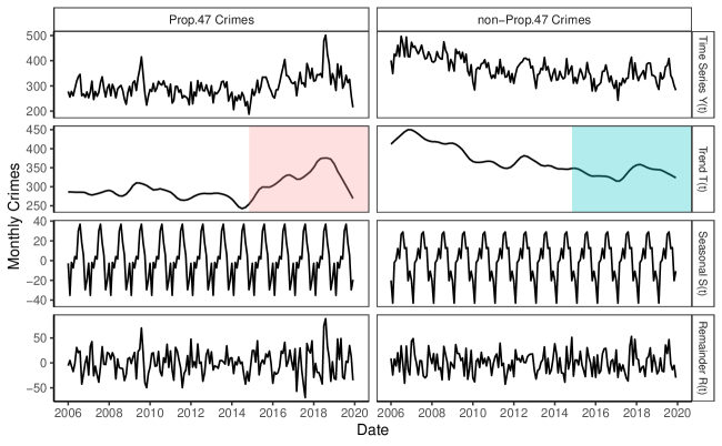
Figure 5: Results from the Seasonal and Trend decomposition using Loess (STL) with an additive model for monthly crimes between 2006-2019. The full time series of crimes per month $Y(t)$ is separated into trend $T(t)$, seasonality $S(t)$, and remainder $R(t)$ components. In each panel, the top row shows the monthly data $Y(t)$, the second row is the trend $T(t)$ as given by the loess smoothed data without seasonality, the third row contains the seasonal component $S(t)$. Finally, the remainder row contains the residual $R(t)$ with seasonality and trend removed from $Y(t)$. This decomposition is performed for Prop. 47 crimes in the left panel and for non-Prop. 47 crimes in the right panel. Note that an increase in the trend emerges for the Prop. 47 crimes towards the end of 2014, but not for non-Prop. 47 crimes.

3.2 Reclassified crimes increase after implementation of Prop. 47

To further identify differences in the temporal evolution of the reclassified and non-reclassified offenses we analyze the entire 2006-2019 crime time series. Temperature variations, seasonal cycles, and the increased criminal opportunities provided by travel and/or shopping during holiday periods are well-known possible crime influencers (Falk, 1952; McDowall et al., 2012; Lauritsen and White, 2014). Although the climate in the coastal Los Angeles basin is typically mild-to-hot and dry throughout the year, heavy rainfall is concentrated in the months of February and March, potentially affecting crime rates. Similarly, large numbers of tourists visit Santa Monica during the summer. It is thus important to remove seasonal effects from the time series to better understand underlying trends. As mentioned in Sect. 2, the raw data lists the date of each crime; for convenience we aggregate all occurrences by month to produce a crime time series $Y(t)$ where $t$ is a discrete variable that labels each month from January 2006 to December 2019. In order to separate the main trend in crime progression from possible periodic perturbations, we use the Seasonal and Trend decomposition using Loess (STL decomposition) method on our data set (Cleveland et al., 1990). Here, the full crime time series $Y(t)$ is decomposed into a trend $T(t)$, a seasonality $S(t)$, and a remainder $R(t)$ so that $Y(t)=T(t)+S(t)+R(t)$, where $S(t)$ is periodic and $R(t)$ represents any residual fluctuations of $Y(t)$. We discard the multiplicative option where the time series is expressed as a product of its components, $Y(t)=S(t)\,R(t)\,T(t)$, since we expect seasonality effects to remain relatively stable over the temporal arc of our data. We decompose the data using the ‘stl’ function in the R statistical package (R Core Team, 2018). The algorithm requires several parameters to be be specified, including $w_{\rm trend}$, the time-frame over which the data is smoothed. Details are illustrated in Sect. A.1 of the Supplementary Information (SI).

STL decomposition results are shown in Fig. 5, where $Y(t)$ is the number of crimes per month from January 2006 to December 2019 for both Prop. 47 and non-Prop. 47 crimes. The trend of the number of monthly Prop. 47 crimes starts to increase towards the end of 2014, but no corresponding rise is observed for the non-reclassified ones. In fact, non-Prop. 47 crimes appear to be declining from 2014 onwards apart from a slight increase around 2018. This indicates that the rise in the observed reclassified crime trend should not be attributed to a general pattern of increasing crime rates in the city of Santa Monica, rather it suggests that a specific event in late 2014 is responsible for the observed rise in Prop. 47 crimes, without playing any role in the dynamics of the non-Prop. 47 ones. We identify this event with the implementation of the new law. A significant drop in the $T(t)$ trend emerges for Prop. 47 crimes towards the end of 2018, persisting throughout 2019, and concurrent with the several new initiatives undertaken by the SMPD to improve public safety and towards more community-based operations.

Interesting observations can also be inferred from the seasonal component $S(t)$: for both Prop. 47 and non-Prop. 47 crimes the number of offenses increases over spring and summer, reaching a peak in August, then declining through November. Crime rates increase again throughout the end-of-the-year holiday season, in December and January, and decline in February, during the rainy period. Although the main features of the seasonality components $S(t)$ of the reclassified and non-reclassified crimes in Fig. 5 are similar, some differences arise, most notably behaviors in the spring and fall months. These slight discrepancies might be ascribed to some crimes being more affected by seasonal changes than others.

3.3 A change-point in the reclassified crime trend occurs in late 2014

Having isolated the trend component $T(t)$ from the time series $Y(t)$, we determine whether any statistically significant changes in $T(t)$ arise. If so, we also aim to identify the times at which these changes occur, and the associated confidence intervals. To do this, we use change-point analysis, a well developed method that has been applied to many disciplines, from economics to medicine (Page, 1954, 1957; Chen and Gupta, 2011). Once a time series is given, the basic foundation of change-point analysis is to evaluate a statistical quantity on a subsample of the data immediately prior and immediately after each time point. If the difference between the prior and after quantities surpasses a given threshold, the selected time point is the locus of a change-point, given that some consistency requirements are met. This concept can be applied to the mean, variance, or any moment or derived property of the data (Killick and Eckley, 2014; Killick et al., 2016). Operationally, the detection of a change-point is framed as a hypothesis test, where the null hypothesis is that there are no change-points and the alternative hypothesis is that at least one exists (Page, 1954, 1957).

Figure 6: Change point analysis on the $M(t)$ slope derived from the $T(t)$ trend for Prop. 47 crimes (left) and non-Prop. 47 crimes (right). The top panels are the $T(t)$ trends derived from the $Y(t)$ monthly data using the smoothing window $w_{\rm trend}=19$ months in the decomposition. The lower panels are the derived $M(t)$ slopes on which change-point analysis is performed after the ‘mosum’ test statistic parameters $G,\eta,\epsilon$ are specified as detailed in the main text and in Sect. A.2 of the SI. For both Prop. 47 and non-Prop. 47 crimes $G=10$ months, $\eta=12$, $\epsilon=0.5$. The left hand panel for reclassified crimes shows a change-point date of July 2014 (dotted line) with a 95% confidence interval between September 2013 and April 2015, which includes November 2014. Most of all other $\{w_{\rm trend},G,\eta,\epsilon\}$ combinations yield a change-point centered towards the latter part of 2014 with a confidence interval that includes November 2014. For the non-reclassified crimes in the right panel, the date of the change-point is October 2006 (dotted line) with a 95% confidence interval between September 2006 and November 2006. Note however, that the non-Prop. 47 change-point is strongly dependent on the specific $\{w_{\rm trend},G,\eta,\epsilon\}$ values chosen and no time-frame emerges that is robust to parameter changes.

In our case, since we expect Prop. 47 to affect the crime trend, we seek to identify the time when $T(t)$ exhibits the largest rate of change. We thus calculate the difference between subsequent $T(t)$ values and derive a new time series for the slope of $T(t)$, which we refer to as $M(t)$. The $M(t)$ time series is constructed by evaluating the backward difference on each time point: if $t_{i-1}<t_{i}$ are consecutive times, we define $M(t_{i})=(T(t_{i})-T(t_{i-1}))/(t_{i}-t_{i-1})$. Since our data points are monthly values, $t_{i}-t_{i-1}=1$ month and $M(t_{i})=(T(t_{i})-T(t_{i-1}))$. We then perform a change-point analysis on $M(t)$ to detect where changes to the slope are largest. We compute $M(t)$ from the trend $T(t)$ rather than from the monthly time series $Y(t)$ because fluctuations in the latter would propagate to the slope, rendering a change-point analysis inconclusive. The trade-off in choosing to work with $T(t)$ rather than $Y(t)$ is that the smoothing process may affect our analysis; for example the change-points may depend on the smoothing window length $w_{\rm trend}$, as discussed in Sect. A.1 of the SI.

Once $w_{\rm trend}$ is selected, the change-points of $M(t)$ are calculated through the R package ‘mosum’ (Meier et al., 2019); the procedure is described in Sect. A.2 of the SI. As illustrated, several parameters must be specified, including the window $G$ over which the prior and after subsamples are evaluated, the minimum allowed distance $\eta G$ between change-points, and the minimum width $\epsilon G$ of a neighborhood of the change-point where the mosum test statistic surpasses the reference threshold for all data points in the $\epsilon G$ neighborhood. These $G,\eta,\epsilon$ parameters affect the location of the change-point and the associated confidence intervals, in addition to $w_{\rm trend}$ from the decomposition.

Results for Prop. 47 and non-Prop. 47 crimes are shown in Fig. 6. The estimated change-point for the Prop. 47 crimes for $w_{\rm trend}=19$ months, $G=10$ months, $\eta=12$, $\epsilon=0.5$ is detected to be July 2014 with a 95% margin of error that includes November 2014. Other choices of $\{w_{\rm trend},G,\eta,\epsilon\}$ yield different change-point estimates, most notably reducing $w_{\rm trend}$ will shift the change-point towards later dates. For example $w_{\rm trend}=5$ months, $G=10$ months, $\eta=10$, $\epsilon=0.5$ yields a change point of August 2014 with a 95% margin of error of ten months, which also includes November 2014. We performed change-point analysis for a large set of $\{w_{\rm trend},G,\eta,\epsilon\}$ combinations. For all of them changes in the rate of Prop. 47 crimes emerged towards the second half of 2014, between June 2014 and August 2014, The choice of $w_{\rm trend}=1$, which corresponds to building the slope $M(t)$ from the full time series $Y(t)$ without any smoothing procedure, typically yields no change-points due to the irregularity of the data, as mentioned above. Some parameter choices allow us to identify additional change-points at the end of 2018. For example, $w_{\rm trend}=19$ months, $G=5$ months, $\eta=5$, $\epsilon=0.5$ yield October 2018 as a new change-point in addition to June 2014. This is true for other $\{w_{\rm trend},G,\eta,\epsilon\}$ combinations that allow for a smaller window size and a smaller distance between change-points. Thus, while the main change-point remains between June 2014 and August 2014, a minor one also arises towards the end of 2018 for Prop. 47 crimes. The change-point loci for the non-Prop. 47 crimes are more heavily dependent on the chosen $\{w_{\rm trend},G,\eta,\epsilon\}$ parameters, and typically do not extend into 2014. In conclusion, most of the parameter combinations tested yield change-point loci for the Prop. 47 crimes that remain within the June 2014 to August 2014 window, with November 2014 falling within the 95% confidence interval in all cases.

3.4 A breakpoint for Prop. 47 crimes is located at November 2014

We now perform segmented regression on the monthly time series $Y(t)$ and on the trend $T(t)$ of both reclassified and non-reclassified crimes as an alternative method to identify the time at which changes occur in the respective data sets. Segmented regression is typically used when abrupt changes are expected in the relationship between an explanatory and a response variable. This relationship is assumed to be piece-wise linear, with segments separated by so-called breakpoints. Under the assumption of a single breakpoint, an initial guess of its location is made and the response variable is fit to two lines, one before and one after the putative breakpoint with the constraint that the overall fit is continuous at the breakpoint itself. The resulting curve is the first estimate on which nonlinear regression models are iterated through least squares, or weighted least squares, methods until convergence is reached and a breakpoint $t^{*}$ identified. This procedure can be extended to multiple breakpoints.

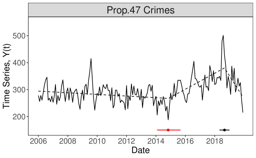
BP 1: Nov 2014 (Feb 2014 - Sept 2015)
BP 2: Sept 2018 (May 2018 - Jan 2019)

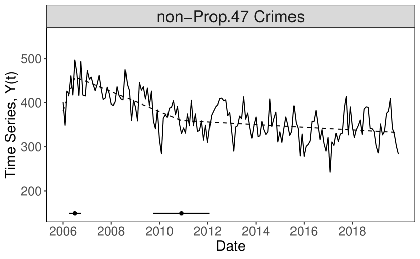
BP 1: Jul 2006 (Apr 2006- Oct 2006)
BP 2: Dec 2010 (Oct 2009 - Feb 2012)

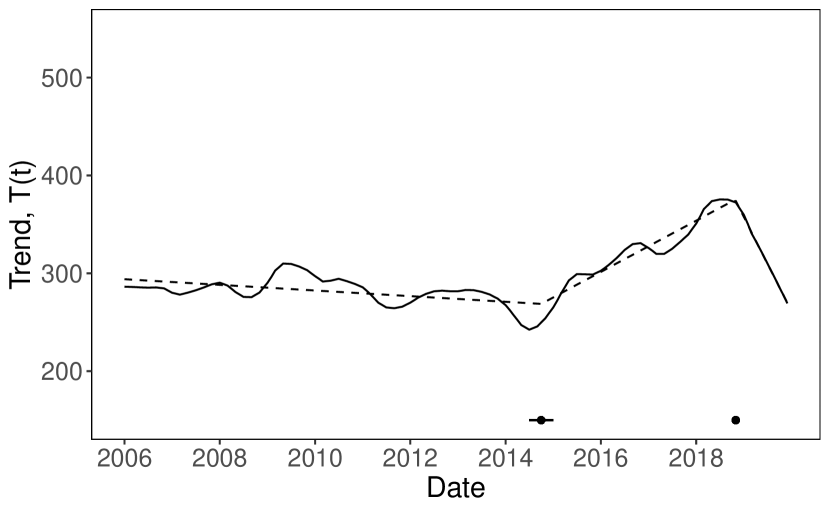
BP 1: Oct 2014 (July 2014 - Jan 2015)
BP 2: Nov 2018 (Oct 2018 - Dec 2018)

BP 1: Nov 2006 (Aug 2006 - Feb 2007)
BP 2: Aug 2010 (Mar 2010 - Jan 2011)

Figure 7: Segmented regression with two breakpoints on $Y(t)$ and $T(t)$ for the reclassified (left) and non-reclassified (right) crimes. The decomposition assumes $w_{\rm trend}=19$ months. Breakpoints (BP) are represented by dots and the respective 95$\%$ confidence intervals are marked by bars; they are both reported in the text below each panel. For the Prop. 47 crimes the first breakpoint is November 2014 for $Y(t)$, and October 2014 for $T(t)$. Values of $1<w_{\rm trend}<19$ months preserve the $T(t)$ breakpoint. The second breakpoint is September 2018 for $Y(t)$, and November 2018 for $T(t)$. The first breakpoint signals a transition to higher crime for both $Y(t)$ and $T(t)$, the second one a decrease. For the non-Prop. 47 crimes, breakpoint dates are highly unstable and sensitive to changes in $w_{\rm trend}$.

We use the R package ‘segmented’ (Muggeo, 2008) to perform segmented regression on $Y(t)$ for Prop. 47 crimes, and on the corresponding $T(t)$ obtained by setting $w_{\rm trend}=19$ months. Since a visual inspection of $T(t)$ reveals at least two possible major changes occurring between 2014 and 2015 and between 2018 and 2019, we impose two breakpoints to the algorithm. Results are shown in Figs. 7. As can be seen, November 2014 emerges as one of the breakpoints for the monthly time series $Y(t)$; the corresponding trend $T(t)$ yields October 2014 as a breakpoint with a 95$\%$ confidence interval that includes November 2014. The location of the $T(t)$ breakpoint is relatively stable: lower values of $1<w_{\rm trend}<19$ months still yield October 2014 as breakpoint. The second breakpoint for $Y(t)$ is September 2018; for $T(t)$ and $w_{\rm trend}=19$ months it is November 2018. Lower values of $w_{\rm trend}$ preserve the November 2018 breakpoint, however $w_{\rm trend}=3$ and 5 months yield September 2018. If we allow for one or three breakpoints, results are highly unstable, with the breakpoint dates changing with each algorithm run. This behavior is indicative of poor a priori assumptions on the number of breakpoints (Bang et al., 2006).

Finally, we perform a segmented regression analysis on the non-Prop. 47 crimes by similarly allowing for two breakpoints. As shown in Fig. 7 when using the monthly time series $Y(t)$, breakpoints occur on December 2016 and August 2019 with 95$\%$ confidence intervals that do not contain November 2014. Performing a segmented regression on $T(t)$ obtained by setting $w_{\rm trend}=19$ months yields one breakpoint on November 2006 and one on August 2010 with 95$\%$ confidence intervals that do not include November 2014 in either case. For the non-Prop. 47 crimes, breakpoints for both $Y(t)$ and $T(t)$ are highly unstable and highly sensitive to the choice of $w_{\rm trend}$. Furthermore, regardless of the value of $w_{\rm trend}$ or the number of breakpoints specified, we found no 95$\%$ confidence interval that contain November 2014, or even a proximal time frame, as a likely breakpoint for non-Prop. 47 crimes. Hence, the abrupt change in the reclassified time series observed in November 2014 should be attributed not to an overall increase in crime, but rather to an event that specifically affected this category of crimes. As discussed above, we identify this event with the implementation of Prop. 47 in November 2014. Similarly, the second breakpoint evaluated on the Prop. 47 time series and occurring in September 2018 may be attributed to the new SMPD policing strategies Renaud, (2019); Pauker, 2019a ; Pauker, 2019b which may have had a stronger impact on Prop. 47 crimes than on non-Prop. 47 ones, for which no corresponding breakpoint was observed. This is because reclassified crimes are generally low-level and quality of life offenses, more easily impacted by the community-based initiatives and the increased patrolling efforts undertaken by the SMPD, such as engagement with vulnerable populations, increased illumination, and physical presence.

4 Neighborhood effects

The city of Santa Monica is divided into eight neighborhoods marked by specific boundaries as shown in the map in Fig. 8. These are: North of Montana, Wilshire/Montana, Northeast Neighbors Association, Mid City, Pico, Downtown, Sunset Park, and Ocean Park. To investigate the geographic effects of Prop. 47, we focus on the before and after Prop. 47 incidence of crime in the above districts and plot the average number of crimes per year for the reclassified and non-reclassified crimes in each neighborhood. The gray bars represent the annual number of crimes before November 2014 and the colored ones those after November 2014, with the color-coding mirroring that of the neighborhood map.

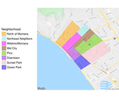
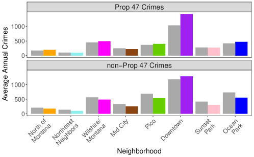
Figure 8: (Top) Color-coding of the eight neighborhoods of the city of Santa Monica. To the north is Pacific Palisades, to the south Venice, to the east West Los Angeles, which are all part of the city of Los Angeles proper. To the west is the Pacific Ocean. (Bottom): Average yearly number of crimes in each neighborhood for Prop. 47 crimes (top) and non-Prop. 47 crimes (bottom). Gray bars indicate the average prior to implementation of the new law in November 2014; the color-coded bars represent the averages after Prop. 47 came into effect.

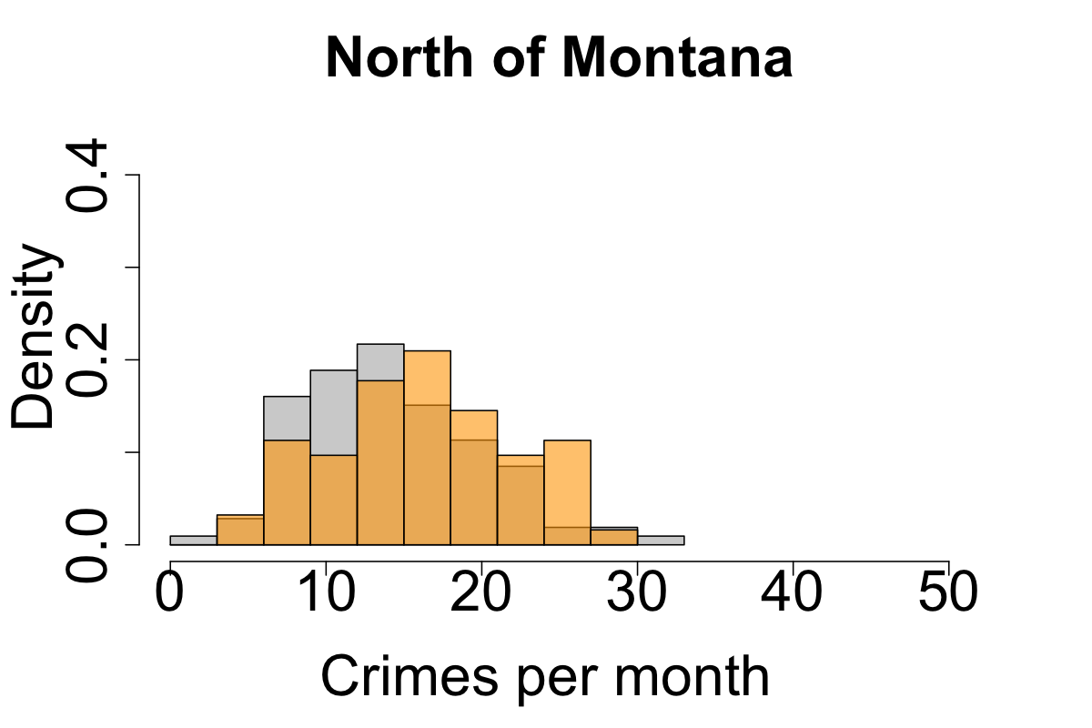
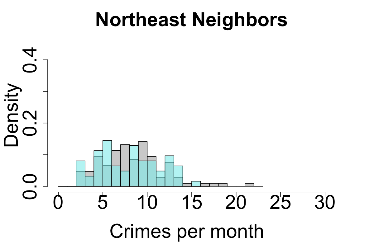
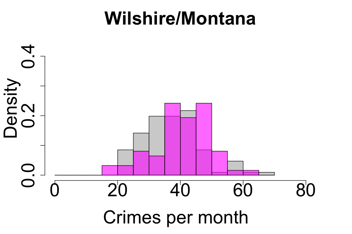
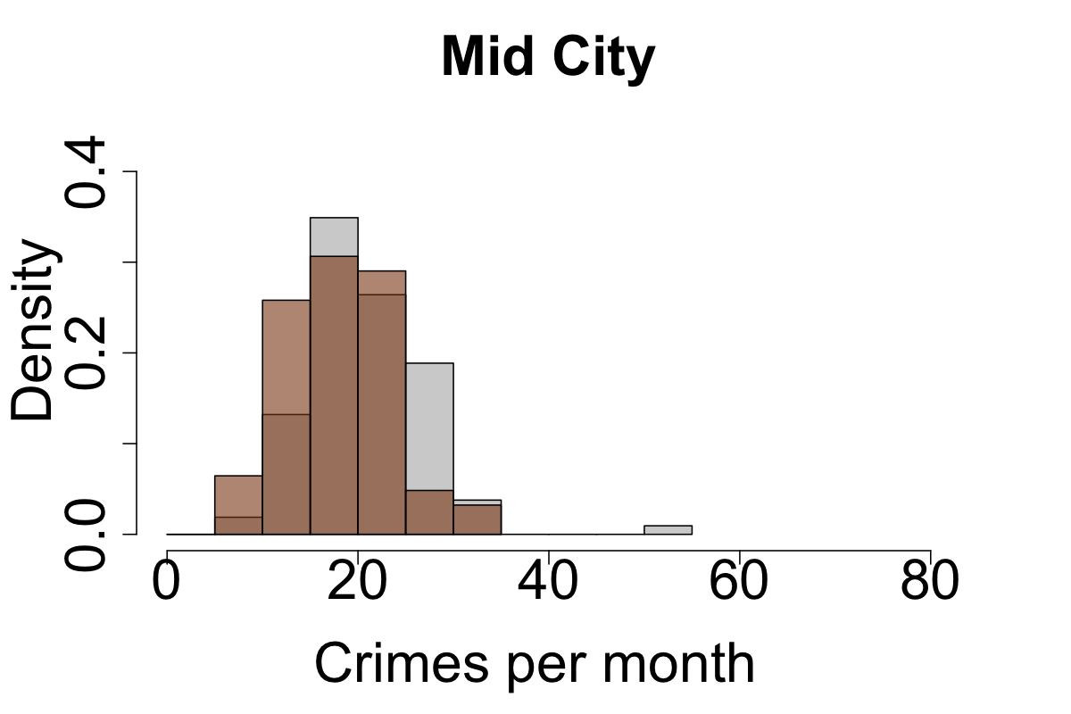
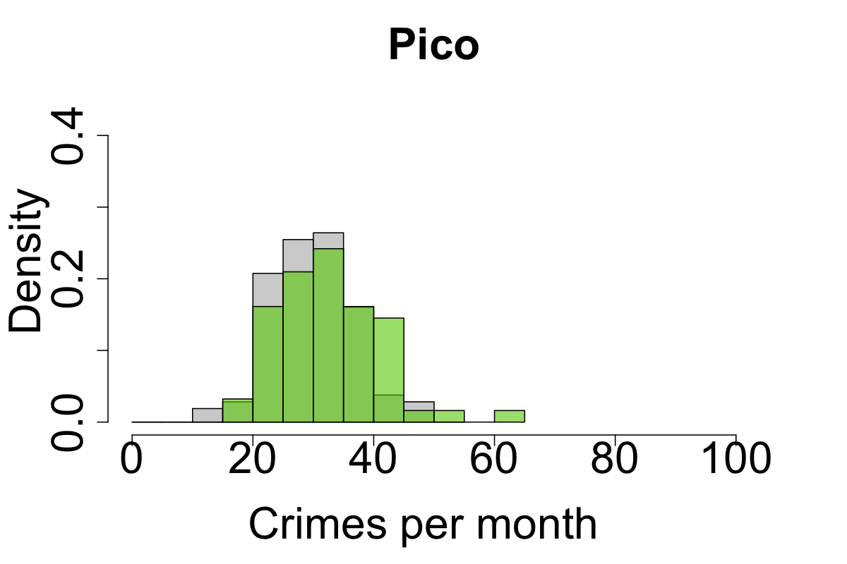
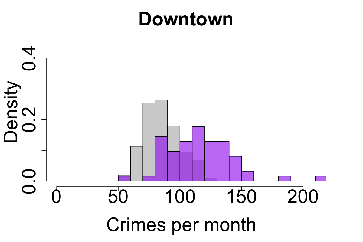
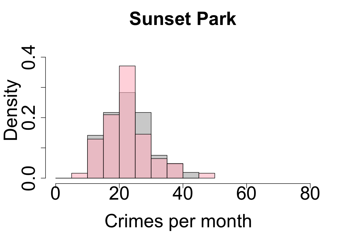
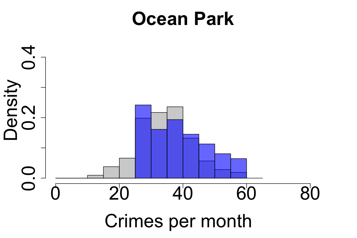
Prop. 47 crimes; Monthly averages

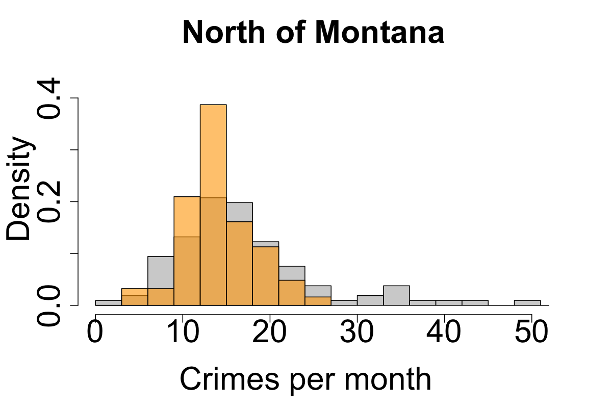
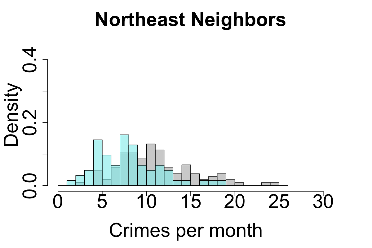
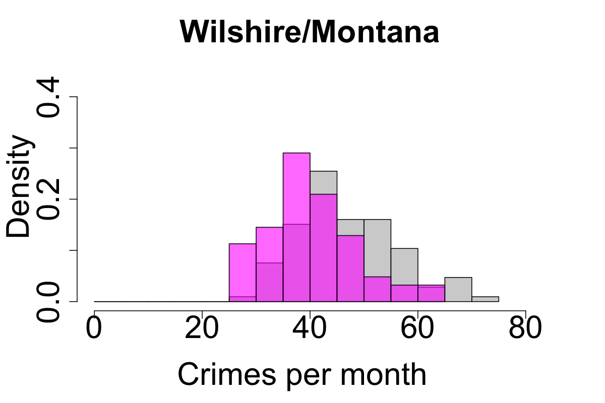
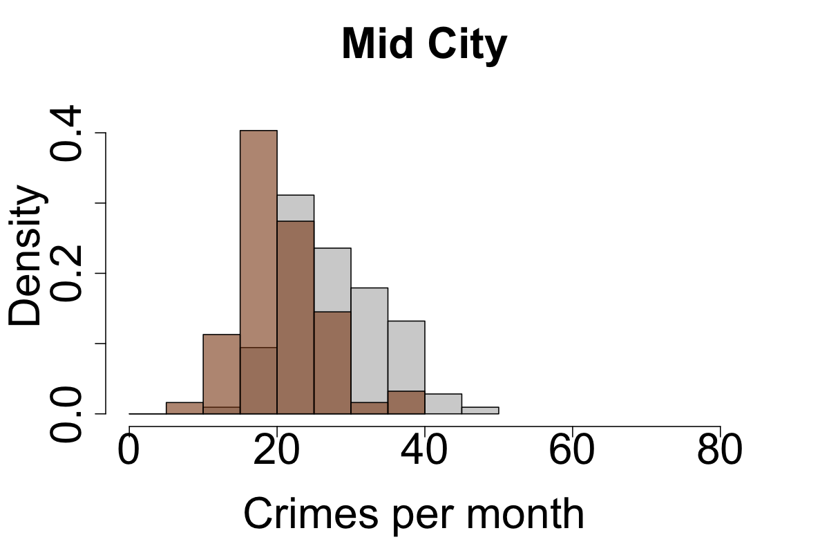
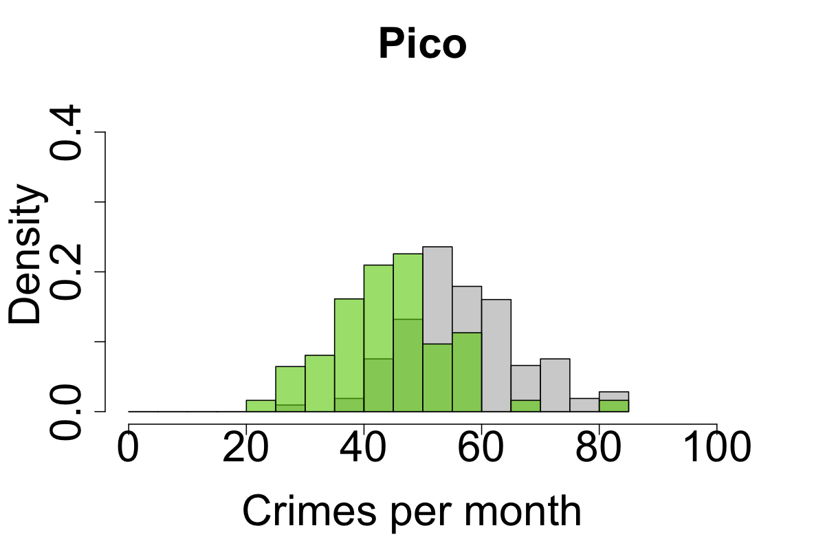
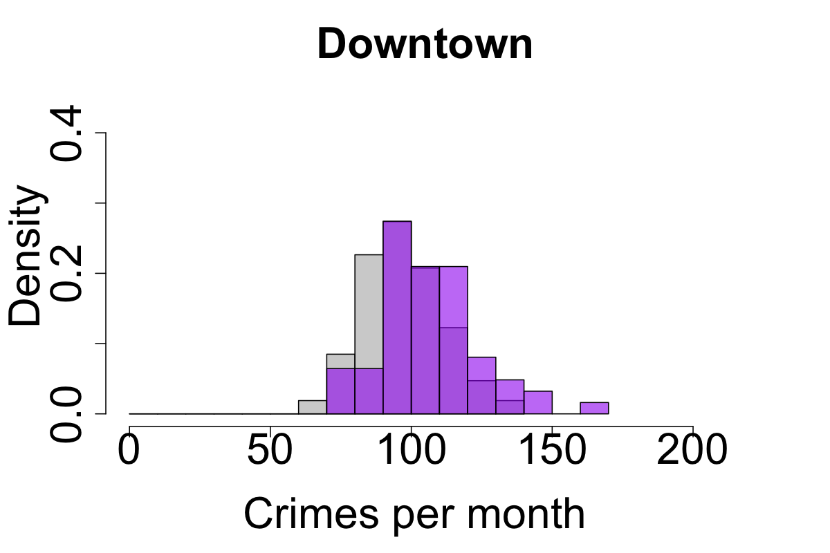
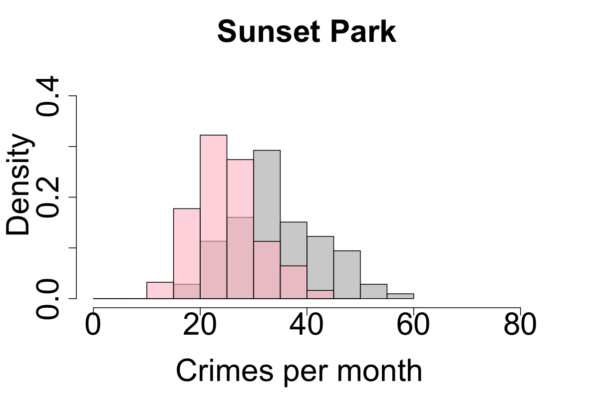
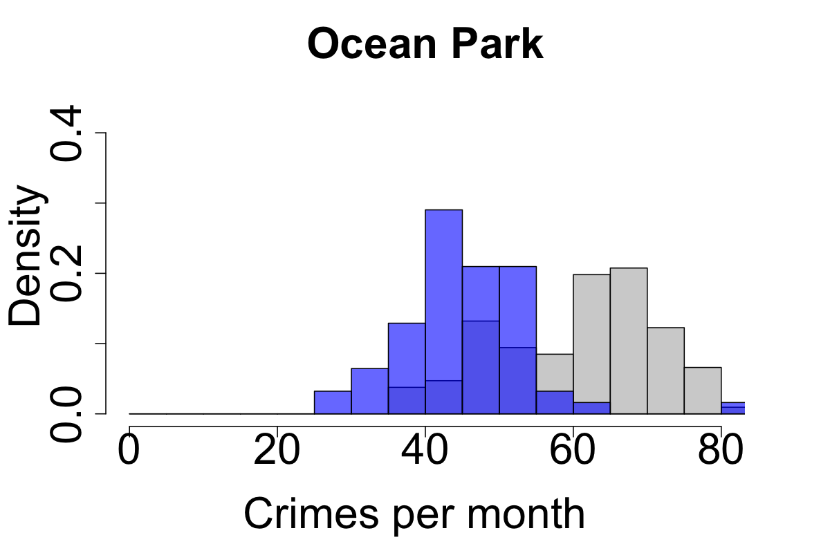
non-Prop. 47 crimes; Monthly averages

Figure 9: Histograms of the number of Prop. 47 (top) and non-Prop. 47 (bottom) monthly crimes in the eight Santa Monica neighborhoods. The gray bars indicate crimes that occurred before November 2014; the colored ones those that occurred after November 2014. Table 2 provides summary statistics.

Prop. 47 crimes; Monthly averages

Neighborhood	Before $\{\mu_{\rm b},\sigma_{\rm b}\}$	After $\{\mu_{\rm a},\sigma_{\rm a}\}$	$t$	Significant?
North of Montana	{14.64, 5.71}	{16.57, 6.02}	2.04	yes, up +13.2$\%$
Wilshire/Montana	{37.75, 9.16}	{41.07, 9.63}	2.20	yes, up +8.8$\%$
Northeast Neighbors	{8.84, 3.55}	{8.50, 3.44}	0.62	no
Mid City	{21.08, 6.03}	{18.62, 5.59}	2.67	yes, down -11.7$\%$
Pico	{30.64, 6.92}	{33.61, 8.37}	2.36	yes, up +9.7$\%$
Downtown	{86.48, 14.59}	{118.69, 29.31}	8.09	yes, up +37.2$\%$
Sunset Park	{23.37, 6.92}	{22.88, 7.49}	0.42	no
Ocean Park	{35.07, 8.44}	{39.27, 9.32}	2.92	yes, up +12.0$\%$

non-Prop. 47 crimes; Monthly averages

Neighborhood	Before $\{\mu_{\rm b},\sigma_{\rm b}\}$	After $\{\mu_{\rm a},\sigma_{\rm a}\}$	$t$	Significant?
North of Montana	{17.52, 8.24}	{14.82, 4.13}	2.82	yes, down -15.4$\%$
Wilshire/Montana	{47.17, 9.34}	{40.67, 8.18}	4.71	yes, down -13.8$\%$
Northeast Neighbors	{11.64, 4.24}	{8.45, 3.63}	5.17	yes, down -27.4$\%$
Mid City	{28.14, 6.86}	{21.08, 5.48}	7.33	yes, down -25.1$\%$
Pico	{57.20, 10.26}	{44.72, 10.04}	7.71	yes, down -21.8$\%$
Downtown	{98.29, 14.15}	{107.00, 17.70}	3.30	yes, up +8.9$\%$
Sunset Park	{34.92, 8.38}	{25.50, 6.60}	8.05	yes, down -27.0$\%$
Ocean Park	{61.08, 10.81}	{46.18, 8.59}	9.84	yes, down -24.4$\%$

Table 2: The Welch’s t-test applied to the histograms of the Santa Monica neighborhoods shown in Fig. 9 for Prop. 47 (top) and non-Prop. 47 (bottom) crimes. The last column indicates whether changes are statistically significant and shows percent changes to the mean. The $\{\mu_{\rm b},\sigma_{\rm b}\}$ quantities are monthly averages and standard deviations of crime before implementation of Prop. 47 calculated over $N_{\rm b}=106$ months. Their post-implementation counterparts are $\{\mu_{\rm a},\sigma_{\rm a}\}$ calculated over $N_{\rm a}=62$ months. The Welch’s t-test statistic, $t$, is compared to the Student’s t-distribution reference value $t_{\rm s}=1.66$. See Sect. 3.1 for more details.

In five of the eight neighborhoods the number of reclassified crimes increased substantially after implementation of Prop. 47, whereas in the other three, the increase was more modest or a small decrease was observed. Changes to the occurrence of non-Prop. 47 crimes after November 2014 are also neighborhood-dependent, but typically involve significant decreases. More quantitatively, we find that the most impacted areas are the Downtown, North of Montana, and Ocean Park neighborhoods which saw the greatest increase in the number of Prop. 47 crimes per year with 37.5$\%$, 13.4$\%$, and 12.2$\%$ increases after implementation of Prop. 47, respectively. Note that North of Montana has total crime counts that are much lower relative to the Downtown and the Ocean Park neighborhoods as can be seen in Fig. 8. Non-Prop. 47 crimes decreased in all areas, except for Downtown where crimes increase by an average of 8.9$\%$ per year.

Similarly to the city-wide analysis carried out in Sect. 3.1, for each of the eight neighborhoods we construct histograms of the average monthly crime rate before and after implementation of Prop. 47 for both reclassified and non-reclassified crimes. Results for all neighborhoods are shown in Fig. 9 for both Prop. 47 and non-Prop. 47 crimes, where gray bars indicate crimes occurring prior to November 2014 and colored bars represent those that occurred after November 2014. We use the same color scheme as in Fig. 8. In all districts, histograms for the Prop. 47 crimes shift to the right or remain unchanged, indicating an increase or stationarity, whereas outcomes for the non-reclassified crimes may shift to the left, indicating a decrease. The only exception is Downtown, where the non-Prop. 47 crime distribution also shifts to the right, indicating an increase.

In Table 2 we quantify whether these shifts are statistically significant by performing a Welch’s t-test in all neighborhoods for both reclassified and non-reclassified crimes. The increases of Prop. 47 monthly crimes in Downtown, North of Montana, Ocean Park, Pico, Wilshire/Montana neighborhoods are large and statistically significant. On the other hand, we observe statistically-significant decreases in non-reclassified crimes in all neighborhoods except Downtown, where we see a modest increase in crime per month. Overall we observe the largest effects of Prop. 47 occur Downtown, where the average monthly incidence of reclassified crimes increased by $37.2\%$ after implementation of the new law. This is to be expected as most of the reclassified crimes are crimes of opportunity and Downtown Santa Monica is rich in crime generators such as shopping, entertainment, and dining venues that attract large numbers of residents and tourists, but also potential offenders due to the ample opportunities for crime these settings offer (Brantingham and Brantingham, 1995). The current analysis reveals that while increased crime levels were observed for the reclassified crimes in most neighborhoods, the strongest effects were felt in areas that were already primed for a criminal surge.

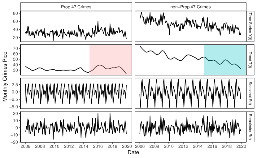
Pico

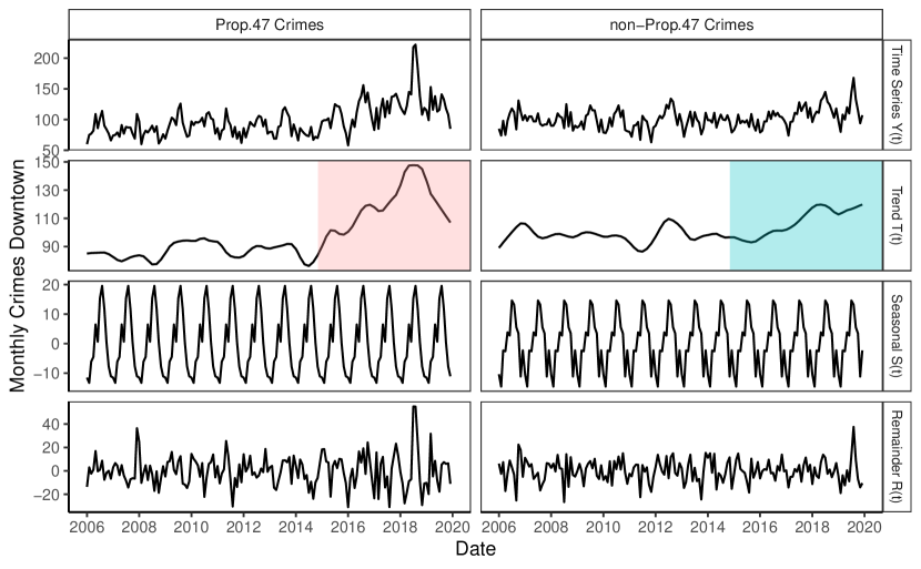
 Downtown

Figure 18: STL decomposition for monthly crimes from 2006 to 2019 in the Downtown and Pico neighborhoods. Prop. 47 (non-Prop. 47) crimes are to the left (right).

In Sect. A.3 we perform an STL decomposition in each of the eight Santa Monica neighborhoods, similarly to what was done in Sect. 3.2 to analyze time dependent trends at the local level. Fig. 18 in the SI shows that Downtown is marked by the highest increase in crime after implementation of Prop. 47 but also by the strongest decrease starting at the end of 2018. The observed decrease may be an indicator of success for the concurrent new police initiatives that added more approachable police officers to engage with the community, often on foot patrol and in highly frequented areas, and a series of measures to improve illumination and monitoring of parking garages and other public places that are more prevalent Downtown.

5 Impacts of the Metro Expo Line light rail extension

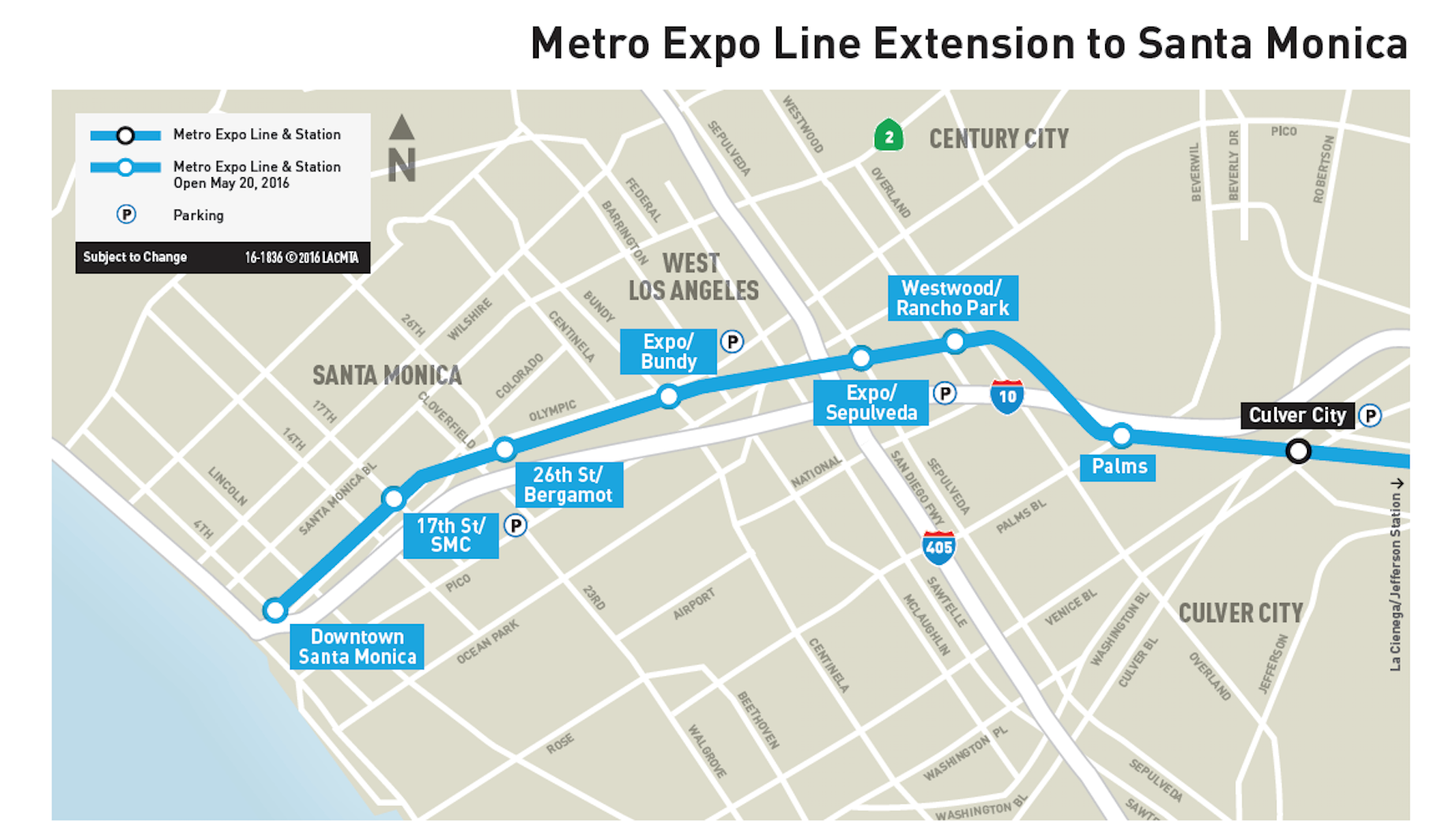
Figure 10: Map of the Metro Expo Line light rail extension to Santa Monica. Operations began on May 20, 2016 at seven new stations, of which four are located within Santa Monica city borders. They are Expo/Bundy, 26^th Street/Bergamot, 17^th Street/Santa Monica College, and Downtown Santa Monica. The other three stations (Palms, Westwood/Rancho Park, Expo/Sepulveda) are within neighboring Culver City. Prior to May 20, 2016 the Expo Line’s terminus was at the Culver City train stop. Picture courtesy of the Los Angeles Metro.

The Metro Expo Line extension was inaugurated on May 20, 2016, connecting Culver City to Santa Monica via light rail. As discussed earlier both the passage of Prop. 47 and the opening of the Expo Line have been inculpated for increases in crime (Cervantes, 2016; Neworth, 2017; Harlander, 2018; Residocracy Santa Monica, 2020; Santa Monica Now, 2020; Santa Monica Crime Watch, 2020). In this section we aim to better understand whether and how the extension of the light rail affected criminal activity around the four new train stations located within Santa Monica municipal borders.

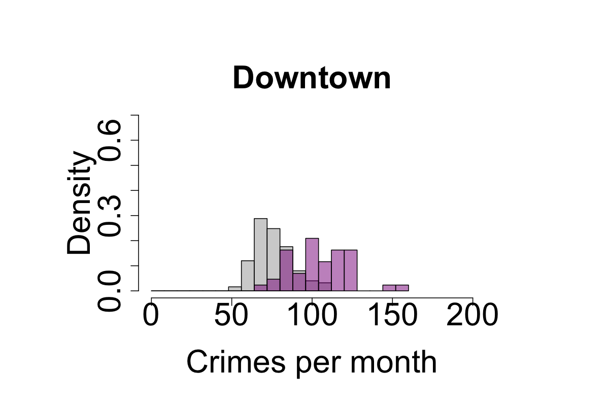
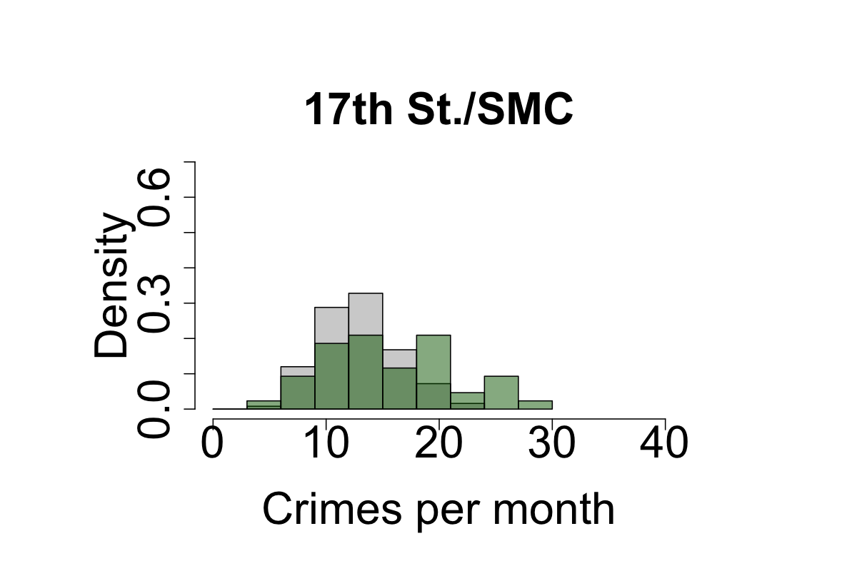
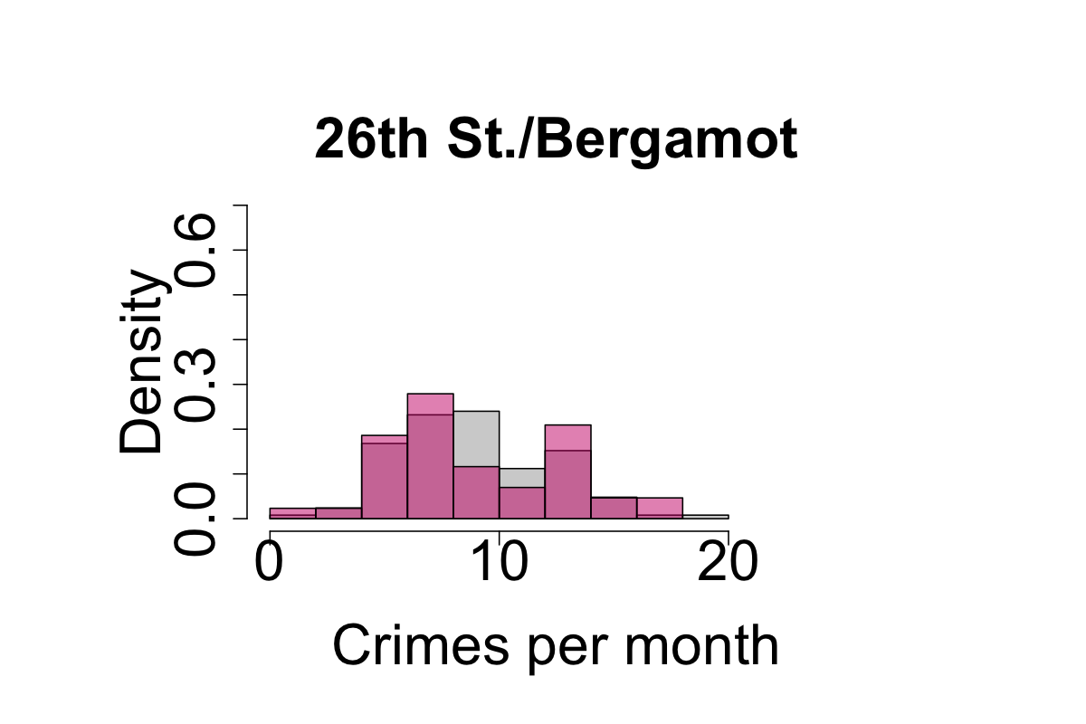
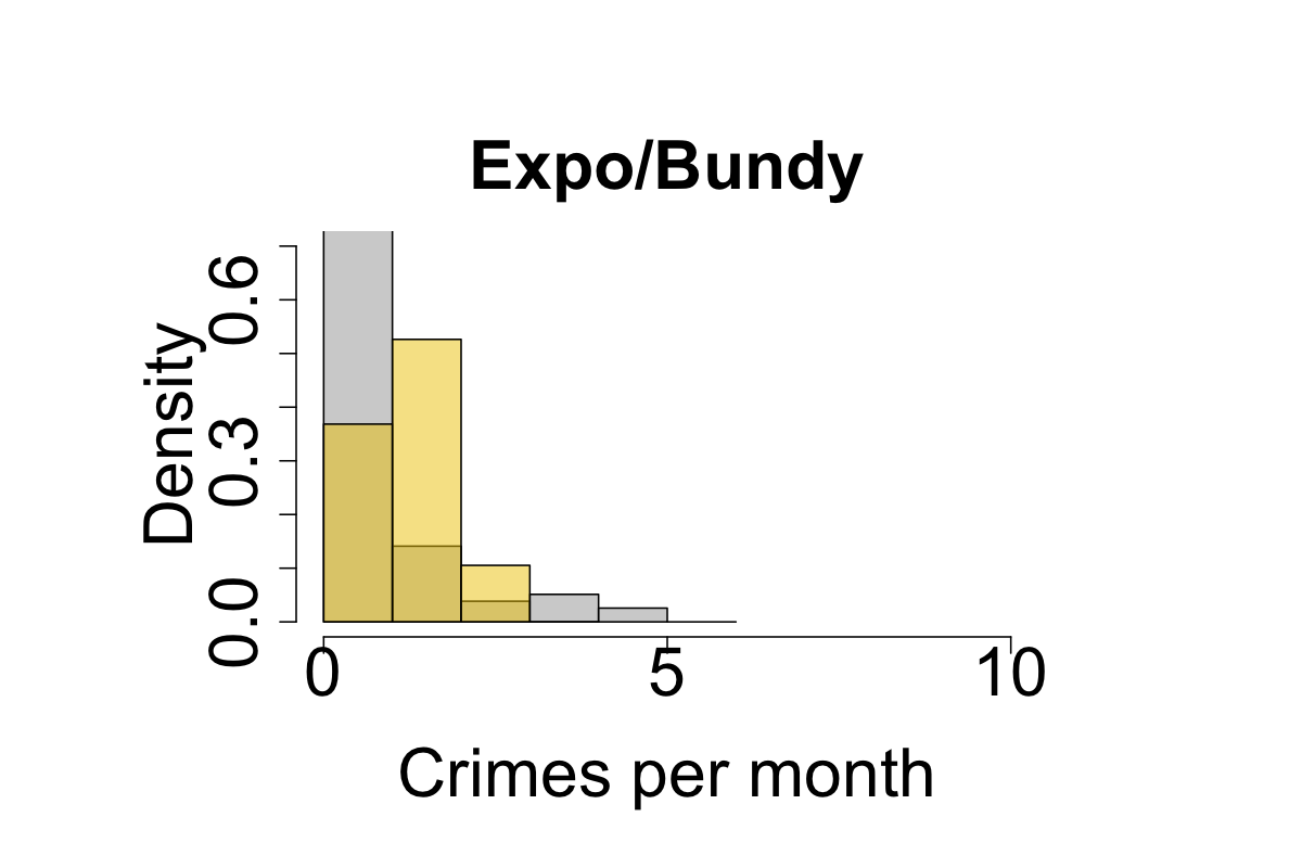
All crimes; Monthly averages before and after the Expo Line (May 2016)

Figure 11: Histograms of monthly total crime counts in a 450 meter radius area centered around the four new Expo Line train stations in Santa Monica. The gray bars represent crime distributions prior to May 2016, the colored ones pertain to data after the same date. Changes to the mean are statistically significant for the Downtown Santa Monica and the 17^th Street/Santa Monica College stations; they are not for 26^th Street/Bergamot and Expo/Bundy. Corresponding data is listed in Table 3.

All crimes; Monthly averages before and after the Expo Line (May 2016)

Train Station	before train	after train	$t,t_{\rm s}$	Significant?
	$\{\mu_{\rm b},\sigma_{\rm b}\}$	$\{\mu_{\rm a},\sigma_{\rm a}\}$
Downtown	{76.51, 12.17}	{105.33, 18.84}	9.38, 1.68	yes, up $+37.7\%$
$17^{th}$ St./SMC	{13.38, 3.55}	{16.07, 5.71}	2.91, 1.68	yes, up $+20.1\%$
26th St./Bergamot	{9.50, 3.21}	{9.63, 3.77}	0.19, 1.67	no
Expo/Bundy	{1.47, 0.98}	{1.74, 0.65}	1.41, 1.68	no

Table 3: The Welch’s t-test applied to the total crime histograms for the Expo Line stations shown in Fig. 11. The last column indicates whether changes are statistically significant and shows percent changes to the mean. The $\{\mu_{\rm b},\sigma_{\rm b}\}$ quantities are monthly averages and standard deviations of crime before inauguration of the Expo Line calculated over $N_{\rm b}=125$ months. Their post-inauguration counterparts are $\{\mu_{\rm a},\sigma_{\rm a}\}$ calculated over $N_{\rm a}=$ 43 months. The Welch’s t-test statistic, $t$, is compared to the Student’s t-distribution reference value $t_{\rm s}$. See Sect. 3.1 for more details.

The possibility of mass transit leading to rising criminal activity, both inside stations and in their immediate vicinity, is well studied. While many studies point to increases in crime (Thrasher and Schnell, 1974; Brantingham et al., 1991; Brantingham and Brantingham, 1993; Poister, 1996; Block and Block, 2000; Ihlanfeldt, 2003), others show that the establishment of mass transit does not necessarily lead to a decline in public safety (Loukaitou-Sideris et al., 2002; Denver Regional Transportation District, 2006; San Diego Association of Governments, 2009). Train and bus routes are usually concentrated in areas with high human activity, offering more opportunities for predatory crime. However, the impact of mass transit on crime is found to also depend on the overall demographic, socio-economic, and land-use contexts surrounding transit stops (Levine et al., 1986; Loukaitou-Sideris, 1999; Loukaitou-Sideris et al., 2002). Thoughtful architectural, lighting, and environmental design of the station themselves may help reduce the incidence of crime (La Vigne, 1996; Felson et al, 1996; Loukaitou-Sideris et al., 2002).

All crimes; Monthly averages (2006-2014; 2014-2016; 2016-2019)

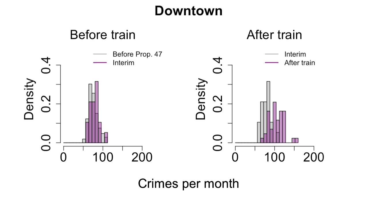
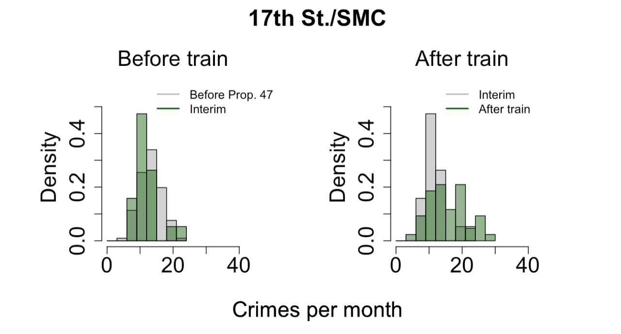
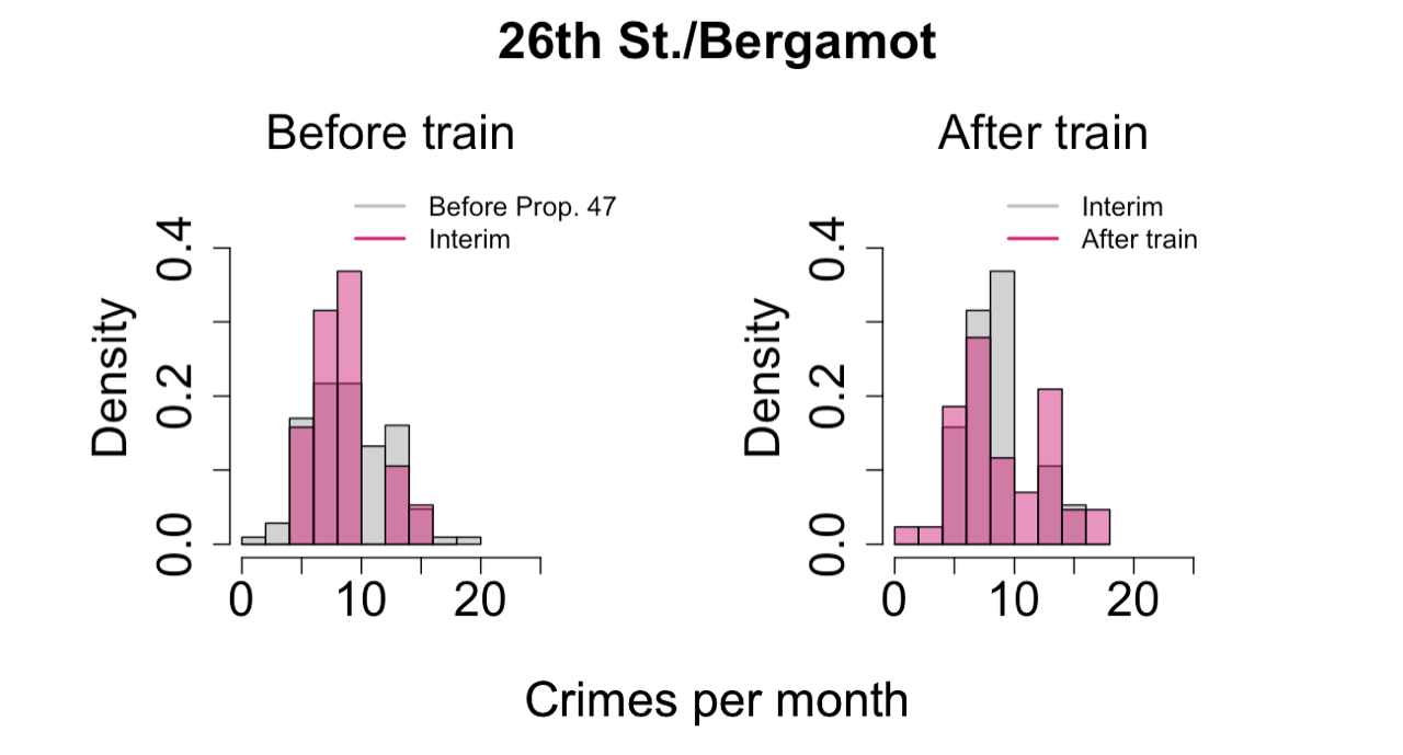
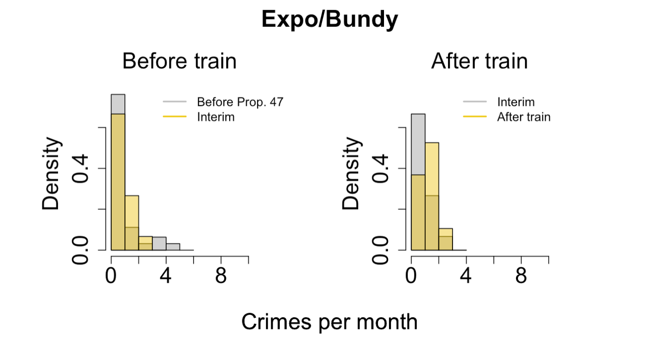
Figure 12: Histograms of monthly total crime counts in a 450 meter radius area centered around the four new Expo Line stations in Santa Monica. In each panel, the left histograms are distributions prior to May 2016 (before and after passage of Prop. 47). Here, the gray and colored bars represent crime densities before passage of Prop. 47, and in the interim between passage of Prop. 47 and before opening of the Expo Line, respectively. The right panels are distributions after November 2014 (before and after opening of the Expo Line). Here, the gray and colored bars represent crime densities in the interim between passage of Prop. 47 and before opening of the Expo Line, and after opening of the Expo Line, respectively. Changes to the mean are not statistically significant prior to opening of the Expo Line; crimes increase significantly at the Downtown and 17^th Street/Santa Monica College stops after opening of the Expo Line. Corresponding data is listed in Table 4.

All crimes; Monthly averages (2006-2014; 2014-2016)

Train Station	before Prop. 47	after Prop. 47	$t,t_{\rm s}$	Significant?
	$\{\mu_{\rm b},\sigma_{\rm b},N_{\rm b}=106\}$	$\{\mu_{\rm a},\sigma_{\rm a},N_{\rm a}=19\}$
Downtown	{75.97, 11.96}	{79.53, 13.23}	1.09, 1.71	no
$17^{th}$ St./SMC	{13.52, 3.49}	{12.58, 3.86}	0.99, 1.71	no
26th St./Bergamot	{9.57, 3.30}	{9.16, 2.67}	0.59, 1.70	no
Expo/Bundy	{0.87, 0.93}	{1.11, 0.60}	1.32, 1.70	N/A

All crimes; Monthly averages (2014-2016; 2016-2019)

Train Station	Before light rail	After light rail	$t,t_{\rm s}$	Significant?
	$\{\mu_{\rm b},\sigma_{\rm b},N_{\rm b}=19\}$	$\{\mu_{\rm a},\sigma_{\rm a},N_{\rm a}=43\}$
Downtown	{79.53, 13.23}	{105.33, 18.84}	6.17, 1.68	yes, up $+32.4\%$
$17^{th}$ St./SMC	{12.58, 3.86}	{16.07, 5.71}	2.81, 1.68	yes, up $+27.7\%$
26th St./Bergamot	{9.16, 2.67}	{9.63, 3.77}	0.56, 1.68	no
Expo/Bundy	{1.11, 0.60}	{0.77, 0.77}	1.86, 1.68	N/A

Table 4: The Welch’s t-test applied to the total crime histograms for the Expo Line stations shown in Fig. 12. The last column indicates whether changes are statistically significant and shows percent changes to the mean. The $\{\mu_{\rm b},\sigma_{\rm b}\}$ quantities are monthly averages and standard deviations of crime before inauguration of the Expo Line calculated over $N_{\rm b}$ months. Their post-inauguration counterparts are $\{\mu_{\rm a},\sigma_{\rm a}\}$ calculated over $N_{\rm a}$ months. The Welch’s t-test statistic, $t$, is compared to the Student’s t-distribution reference value $t_{\rm s}$. There is not sufficient data for meaningful conclusions at Expo/Bundy. See Sect. 3.1 for more details.

To understand whether and how the extension of the Expo Line impacted crime rates in the vicinity of the four new train stations in Santa Monica we consider crime count distributions within a circle of radius 450 meters centered around the four new Expo Line stops. A detailed map is shown in Fig. 10. We first neglect passage of Prop. 47 and consider the total crime distribution before and after inauguration of the light rail extension on May 20, 2016. For simplicity, we categorize the entire month of May 2016 as falling before opening of the Expo Line when creating monthly aggregates. Results are shown in Fig. 11 and in Table  3. The crime distributions shift to the right in a statistically significantly manner after opening of the Expo Line at the Downtown Santa Monica and the 17^th Street/Santa Monica College stops. These shifts correspond to $37.7\%$ and $20.1\%$ increases in monthly crime rates, respectively. No statistically significant changes are observed around the 26^th Street/Bergamot and the Expo/Bundy stations, which are located in areas with fewer crime attractors and human activity compared to the other two, and where the average number of monthly crimes is also much lower in comparison.

To separate the impacts of Prop. 47 from the opening of the Expo Line we further refine our data by binning it into three time periods: January 2006–October 2014 (before implementation of Prop. 47); November 2014–May 2016 (between the implementation of Prop. 47 and the opening of the Expo Line); June 2016–December 2019 (after the opening of the Expo Line). As a result of this stratification, only one or less crimes per month emerge at the Expo/Bundy stop. Given the paucity of data, we do not perform any further statistical analysis on this station. As seen in Fig. 12 and in Table 4, there is no significant increase in the number of overall monthly crimes near any of the other transit stops immediately after passage of Prop. 47 and prior to opening of the Expo Line (2014-2016). Total crimes instead increase dramatically after opening of the Expo Line at the Downtown and 17^th Street/Santa Monica College stops by $32.4\%$ and 27.7% respectively. Upon restricting our analysis to the reclassified crimes, as shown in Fig. 13 and in Table 5, we find that Prop. 47 crimes increased significantly not only at the Downtown and 17^th Street/Santa Monica College stops, but also at 26^th Street/Bergamot by $30.6\%$, $38.6\%$, and 30.0$\%$ respectively. Finally, non-Prop. 47 crimes increased at the Downtown and 17^th Street/Santa Monica College stops by $34.6\%$ and $20.6\%$, respectively, but did not affect 26^th Street/Bergamot.

Prop. 47 crimes; Monthly averages (2006-2014; 2014-2016; 2016-2019)

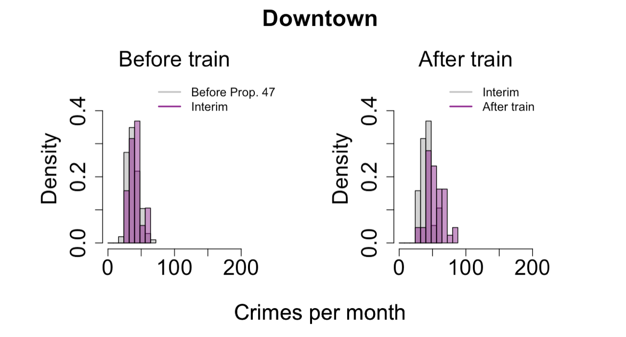
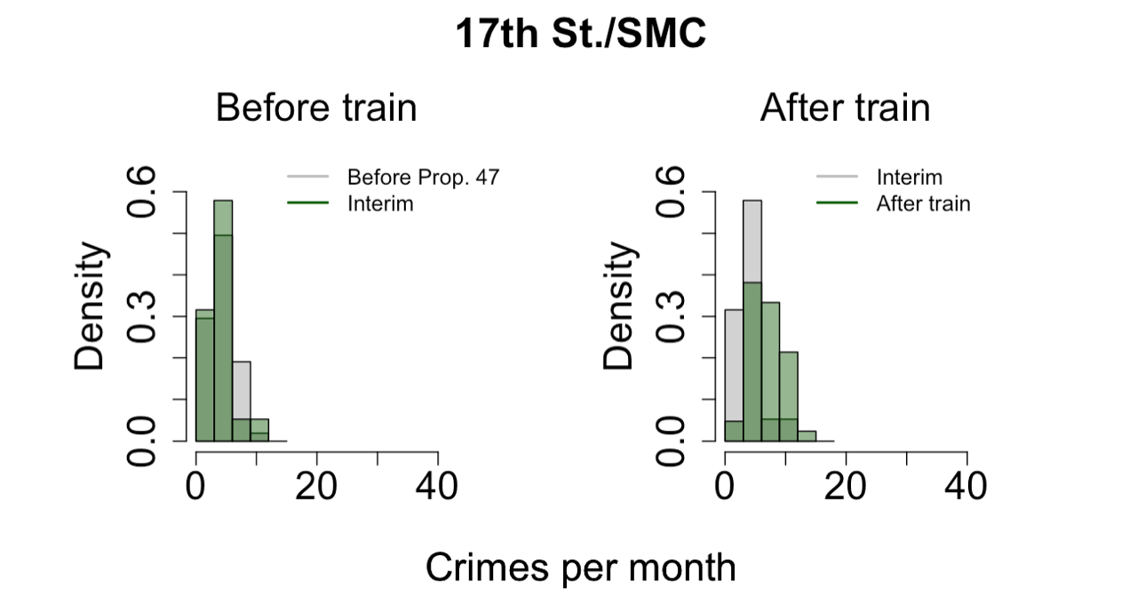
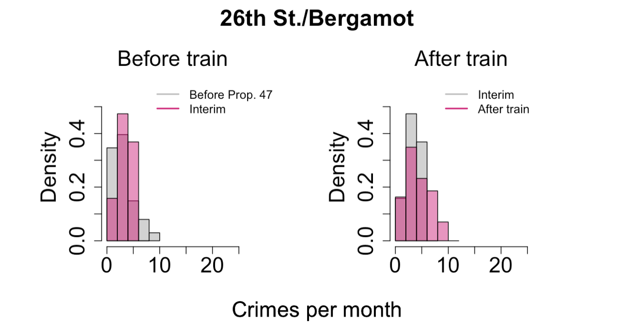
Figure 13: Histograms of monthly Prop. 47 crime counts in a 450 meter radius centered around the four new Expo Line stations in Santa Monica. In each panel, the left histograms are distributions prior to May 2016 (before and after passage of Prop. 47). Here, the gray and colored bars represent crime densities before passage of Prop. 47, and in the interim between passage of Prop. 47 and before opening of the Expo Line, respectively. The right panels are distributions after November 2014 (before and after opening of the Expo Line). Here, the gray and colored bars represent crime densities in the interim between passage of Prop. 47 and before opening of the Expo Line, and after opening of the Expo Line, respectively. Not enough events are recorded at Expo/Bundy for a meaningful analysis. Changes to the mean are not statistically significant prior to opening of the Expo Line; reclassified crimes increase in all stations for which there is sufficient data. Corresponding data is listed in Table 5.

Prop. 47 crimes; Monthly averages (2006-2014; 2014-2016)

Train Station	before Prop. 47	after Prop. 47	$t,t_{\rm s}$	Significant?
	$\{\mu_{\rm b},\sigma_{\rm b},N_{\rm b}=106\}$	$\{\mu_{\rm a},\sigma_{\rm a},N_{\rm a}=19\}$
Downtown	{38.38, 8.93}	{41.47, 8.95}	1.39, 1.71	no
$17^{th}$ St./SMC	{4.74, 2.00}	{5.00, 2.52}	0.44, 1.72	no
26th St./Bergamot	{3.48, 1.90}	{3.74, 1.56}	0.65, 1.70	no
Expo/Bundy	{0.12, 0.31}	{0.21, 0.36}	1.00, 1.72	N/A

Prop. 47 crimes; Monthly averages (2014-2016; 2016-2019)

Train Station	Before light rail	After light rail	$t,t_{\rm s}$	Significant?
	$\{\mu_{\rm b},\sigma_{\rm b},N_{\rm b}=19\}$	$\{\mu_{\rm a},\sigma_{\rm a},N_{\rm a}=43\}$
Downtown	{41.47, 8.95}	{54.14, 12.23}	4.57, 1.71	yes, up $+30.6\%$
$17^{th}$ St./SMC	{5.00, 2.52}	{6.93, 2.74}	2.76, 1.70	yes, up $+38.6\%$
26th St./Bergamot	{3.74, 1.56}	{4.86, 2.41}	2.19, 1.68	yes, up $+30.0\%$
Expo/Bundy	{0.21, 0.36}	{0.23, 0.37}	0.22, 1.70	N/A

Table 5: The Welch’s t-test applied to the Prop. 47 crime histograms for the Expo Line stations shown in Fig. 13. The last column indicates whether changes are statistically significant and shows percent changes to the mean. We consider two time frames, before and after passage of Prop. 47, and before and after inauguration of the Expo Line. The respective before averages and standard deviations $\{\mu_{\rm b},\sigma_{\rm b}\}$ calculated over $N_{\rm b}$ months, and after averages and standard deviations $\{\mu_{\rm a},\sigma_{\rm a}\}$ calculated over $N_{\rm a}$ months, are listed. The Welch’s t-test statistic, $t$, is compared to the Student’s t-distribution reference value $t_{\rm s}$. There is not sufficient data for meaningful conclusions at Expo/Bundy. See Sect. 3.1 for more details.

non-Prop. 47 crimes; Monthly averages (2006-2014; 2014-2016; 2016-2019)

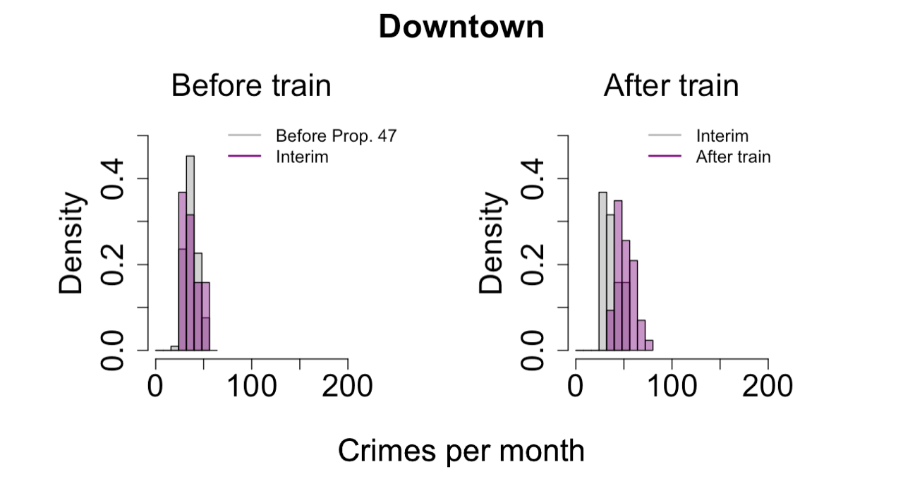
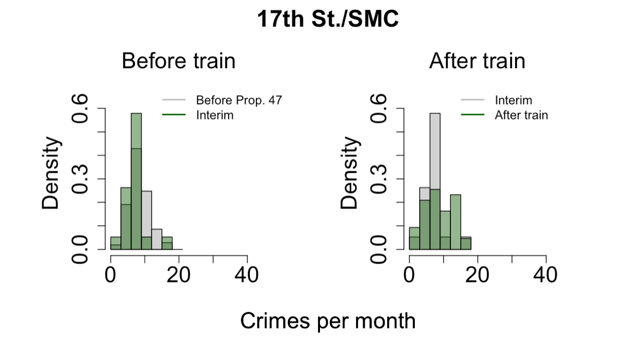
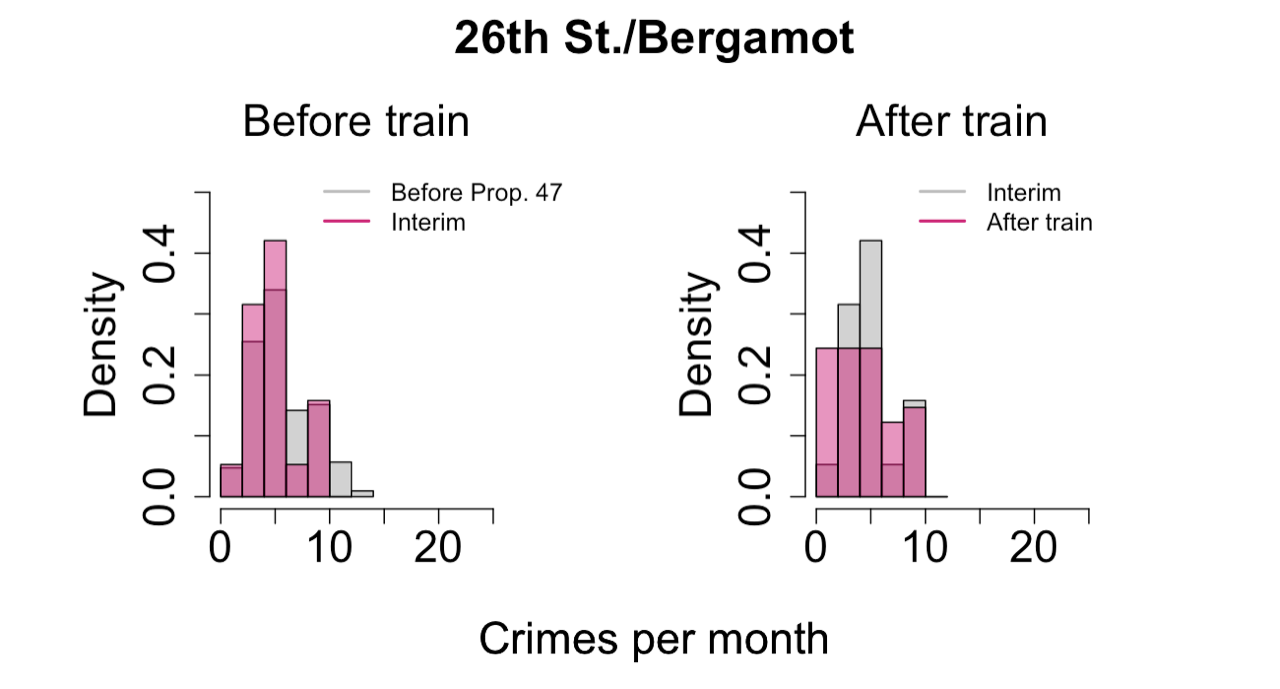
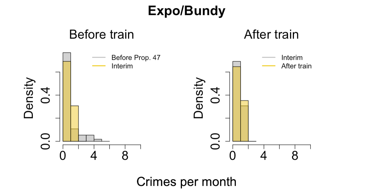
Figure 14: Histograms of monthly non-Prop. 47 crime counts in a 450 meter radius centered around the four new Expo Line stations in Santa Monica. In each panel, the left histograms represent distributions prior to May 2016 (before and after passage of Prop. 47). Here, the gray and colored bars represent crime densities before passage of Prop. 47, and in the interim between passage of Prop. 47 and before opening of the Expo Line, respectively. The right panels are distributions after November 2014 (before and after opening of the Expo Line). Here, the gray and colored bars represent crime densities in the interim between passage of Prop. 47 and before opening of the Expo Line, and after opening of the Expo Line, respectively. Not enough events are recorded at Expo/Bundy for a meaningful analysis. The mean decreases or stays constant both prior and after opening of the Expo Line, except for Downtown and 17^th Street/Santa Monica College where non-Prop. 47 crimes increased after opening of the Expo Line. Corresponding data is listed in Table 6.

non-Prop. 47 crimes; Monthly averages (2006-2014; 2014-2016)

Train Station	before Prop. 47	after Prop. 47	$t,t_{\rm s}$	Significant?
	$\{\mu_{\rm b},\sigma_{\rm b},N_{\rm b}=106\}$	$\{\mu_{\rm a},\sigma_{\rm a},N_{\rm a}=19\}$
Downtown	{37.59, 6.7}	{38.05, 7.49}	0.25, 1.71	no
$17^{th}$ St./SMC	{8.78, 3.02}	{7.58, 2.69}	1.80, 1.70	yes, down -13.7$\%$
26th St./Bergamot	{6.08, 2.67}	{5.42, 2.29}	1.13, 1.70	no
Expo/Bundy	{0.76, 0.85}	{0.89, 0.51}	0.91, 1.70	N/A

non-Prop. 47 crimes; Monthly averages (2014-2016; 2016-2019)

Train Station	Before light rail	After light rail	$t,t_{\rm s}$	Significant?
	$\{\mu_{\rm b},\sigma_{\rm b},N_{\rm b}=19\}$	$\{\mu_{\rm a},\sigma_{\rm a},N_{\rm a}=43\}$
Downtown	{38.05, 7.49}	{51.19, 9.4}	5.87, 1.68	yes, up +34.6$\%$
$17^{th}$ St./SMC	{7.58, 2.69}	{9.14, 3.78}	1.85, 1.68	yes, up +20.6$\%$
26th St./Bergamot	{5.42, 2.29}	{4.77, 2.69}	1.00, 1.70	no
Expo/Bundy	{0.89, 0.51}	{0.53, 0.60}	2.42, 1.70	N/A

Table 6: The Welch’s t-test applied to the non-Prop. 47 crime histograms for the Expo Line stations shown in Fig. 14. The last column indicates whether changes are statistically significant and shows percent changes to the mean. We consider two time frames, before and after passage of Prop. 47, and before and after inauguration of the Expo Line. The respective before averages and standard deviations $\{\mu_{\rm b},\sigma_{\rm b}\}$ calculated over $N_{\rm b}$ months, and after averages and standard deviations $\{\mu_{\rm a},\sigma_{\rm a}\}$ calculated over $N_{\rm a}$ months, are listed. The Welch’s t-test statistic, $t$, is compared to the Student’s t-distribution reference value $t_{\rm s}$. There is not sufficient data for meaningful conclusions at Expo/Bundy. See Sect. 3.1 for more details.

Our analysis indicates that the arrival of light rail was accompanied by a surge in the occurrence of crime in proximity of the Downtown Santa Monica stop, where all types of crime, reclassified and non-reclassified, increased by large percentages. Light rail was also accompanied by an increase in Prop. 47 crimes near two of the other three stations ($17^{th}$ Street/Santa Monica College and $26^{th}$ Street/Bergamot), while non-Prop. 47 crimes remained stationary or decreased in all three. Tables 5 and 6 reveal that there were no statistically significant increases in crime after passage of Prop. 47 but before opening of the Expo Line (2006-2016) at any of the four new train stations, including Downtown. This may be due to ongoing construction of the Expo Line, which began in 2011 and was still active when Prop. 47 was implemented so that any associated effects could only emerge after the train began its operations in May 2016. Finally, the interval between November 2014–May 2016 comprises only 18 months and includes one summer and two winters. This period is thus marked by an unbalanced seasonality, which may be reflected in the corresponding monthly averages.

6 Conclusions

Using a publicly-available database compiled and maintained by the Santa Monica Police Department, we investigated whether passage of Proposition 47 in the state of California had any impact on criminal activity. We specifically focused on crimes that were directly affected by legislative change and were reclassified from felonies to misdemeanors. Our analysis shows that overall the monthly count of these crimes (larceny, fraud, possession of narcotics, forgery, receiving/possessing stolen property) increased by about 15$\%$ after implementation of Proposition 47 in November 2014. By contrast, the non-reclassified crime count decreased by 13$\%$ after the new legislation became effective. We used a Welch’s t-test to verify that the reclassified crime distribution shift from less crime before November 2014 to more crime after the same date was statistically significant, as well as signal decomposition to isolate the main crime trends from seasonal effects. Using change-point analysis, we identified a discontinuity in crime trend at the end of 2014. A segmented regression analysis on the monthly time series led us to identify November 2014 as the main breakpoint. We also identified a secondary discontinuity in the crime trend and a secondary break-point in the monthly time series, both occurring towards the end of 2018, indicating a decreases in crime concurrent with the new SMPD policing efforts. While these changes are too recent to reverse the overall crime surge observed after the 2014 implementation of Prop. 47, and while it is unclear what the longer term implications of the new initiatives will be, our results show that community partnerships, a responsive and outward facing police force, and targeted measures, may help ameliorate crime.

We also considered the impact of Prop. 47 on the eight neighborhoods that comprise the city and verified that the largest monthly change in crime (+37.2$\%$) occurred Downtown, an area with many opportunistic crime attractors, such as nightlife, tourists, dining venues, and shopping centers. Finally, we examined the effects of the opening of the Expo Line on monthly crime rates within 450 meters from four new transit stations. We find that total crime counts increase significantly at the Downtown Santa Monica and 17^th Street/Santa Monica College stops. Prop. 47 and non-Prop. 47 percent increases were comparable at the Downtown Santa Monica stop (+30.6$\%$ and +34.6$\%$ respectively); at the 17^th Street/Santa Monica College stop instead, the increase for Prop. 47 crimes (+38.6$\%$) was much higher than for non-Prop. 47 ones (+20.6$\%$).

Several observations are in order. The city of Santa Monica does not report the monetary value of relevant crimes. Partitioning of the data into reclassified vs. non-reclassified offenses is thus based on our best estimate of which crimes would, on average, fall under the 950 USD threshold, one of the conditions specified by Prop. 47 for reclassification. For example, the initiative applies to grand theft auto but only for vehicles worth less than 950 USD. Since the typical value of stolen cars in Santa Monica surpasses this threshold, we do not include grand theft auto in the list of Prop. 47 crimes. It is clear that exceptions may exist and that our partitioning may have introduced errors; however, due to the large data sample, we expect these not to be systematic and not to have significantly affected our results. Other biases could arise from unreported victimizations differentially affecting the reclassified vs. non-reclassified crime categories. For instance, the US Department of Justice estimates that the average annual incidence of unreported larceny was 41$\%$ nationwide over the 2006–2010 period; for motor vehicle theft the same figure was 17$\%$ (Langton et al., 2012). Similarly, reporting rates could change over time in response to changing perceptions of the effectiveness of reporting crimes. We also observe that in the immediate vicinity of the four new train stations in Santa Monica no increases in reclassified or non-reclassified crimes were observed after passage of Prop. 47 but before opening of light rail. This may be due to ongoing construction of the new crime attractor, which delayed the effects of Prop. 47. Indeed, crimes increased dramatically at the busiest transit stations after opening of the Expo Line, especially in the Downtown area and for the reclassified crimes. Finally, the period between passage of Prop. 47 in November 2014 and the opening of the Expo Line in May 2016 is only 18 months. Compounding effects of the two events may have led to the observed increases in crime; disentangling their overlap may require more discriminants than the data analyzed here.

Possible extensions of this work would involve analyzing crime occurrence in neighboring cities that share similar socio-economic backgrounds with Santa Monica, such as Culver City (population 39,000), Pasadena (population 138,000) or Glendale (population 203,000); all within Los Angeles County, although not directly adjacent to the Pacific Ocean and less touristic. Similarly, it would be interesting to study the incidence of crime on the other three new Expo Line stations operating in Culver City (Palms, Westwood/Rancho Park, Expo/Sepulveda) to compare and contrast results between the two municipalities. A longer term monitoring of crime in Santa Monica would also be desirable. On one hand, it would allow us to determine whether the decrease in the number of monthly crimes observed in late 2018 persists or stabilizes over time. On the other, it would allow us to better discern the effects of the Expo Line, since the incidence of crime may temporarily increase around newly opened stations and settle back to their original levels once novelty effects subside (Poister, 1996). This may not be possible due to the COVID-19 pandemic that severely impacted the global economy. Suspension of all non-essential activities and stay-at-home orders within the city of Santa Monica, as well as reduction to service and ridership of the Expo Line, do not allow for a meaningful, continuous, long term analysis. Although conducted over short time frames, both after passage of Prop. 47 and the inauguration of the Expo Line, our results do suggest that neighborhood characteristics may influence crime rates, since areas with more opportunities for crime appear to have been affected more by the light rail extension and by the new law. Similarly, our results show that community-based policing, a stronger police presence and targeted interventions may help reduce crime.

Finally, although we find a rise in reclassified crimes that coincides with passage of Prop. 47, our research does not provide a definite causative explanation for it. While it is possible that the new law directly motivated offenders to commit more reclassified crimes, there may also be other relevant explanations contributing to the rise. Among them, the increased attention of police, heightened public awareness, more reporting, all of which may have been influenced by media coverage. The observed rise may also be a loose manifestation of the well known Hawthorne effect, whereby individuals modify their behavior as a result of being part of an experiment or study (Roethlisberger and Dickson, 1939; Adair, 1984). In this case, reporting behavior could have been affected by awareness of the changes brought by Prop. 47. Similarly, the decrease in the number of reported reclassified crimes observed in late 2018 may be due to shifts in policing, but also due to fading of Prop. 47 awareness, or habituation. We hope that these and other considerations relevant to public utility, respect for human rights, and existence of socioeconomic disparities, will be used in combination with our results to assess the overall effect of Prop. 47.

7 Acknowledgements

We thank the Santa Monica Police Department, Tricia Crane, Michele Modglin and Jude Higdon-Topaz for valuable information and for the generous time spent discussing our work with us. We thank the AMS Mathematics Research Community where this work was initiated. We also thank Hwayeon Ryu for contributing to the beginning stages of this study. Finally, we acknowledge support from the National Science Foundation under grants DMS 1440386 (CV), DMS 1703761 (JC) and from the Army Research Office under grant ARO W911NF-16-1-0165 (MRD).

Appendix A Supplementary Information

A.1 Seasonal and Trend decomposition using Loess (STL)

In our work the decomposition is performed via the ‘stl’ function in the R software environment (R Core Team, 2018) using an iterative process that uses the monthly time series $Y(t)$ as input data and user-specified initial trend and seasonality estimates. The latter are typically null sets. In each iteration the data is cleared of the current trend estimate and broken into cycle-subseries, one for each of the data points within a period. In our case, since we have monthly data with a periodicity of $n_{\rm p}=12$ months, twelve cycle-subseries arise, one for each month. A new seasonal series is obtained through a combination of loess (locally estimated scatterplot smoothing) polynomial regression with given weights, and moving averages performed on each of the cycle-subseries. The loess regression ensures that the obtained seasonality is defined for all times, not just when data points are available; the moving average procedures guarantee the mean is nearly zero. The input data is then cleared of the newly derived seasonal effect and a temporary trend is obtained, once more using a loess polynomial regression. The freshly derived trend and seasonal estimates are then used as inputs for the next iteration. Any residual elements are included in the remainder and used to compute robustness weights, to reduce the influence of transient, aberrant behavior in the data on the trend and seasonal components. The procedure is run until a pre-set convergence is reached; typically two loops suffice.

Figure 15: Trends $T(t)$ evaluated on Prop. 47 crimes using decomposition using loess from the R statistical package with varying window lengths $w_{\rm trend}$. Note that as $w_{\rm trend}$ increases the corresponding $T(t)$ becomes smoother. Unless otherwise stated, we set $w_{\rm trend}=19$ months (black curve) as determined by Eq. (3) throughout this work.

Two window lengths must be specified to apply the loess regression in the ‘stl’ function: $w_{\rm{season}}$ (the s.window argument in R) and $w_{\rm{trend}}$ (the t.window argument in R). Since we do not assume seasonal patterns to have significantly evolved over the thirteen year time span under investigation, we use the entire data to perform the loess seasonal smoothing analysis and set $\rm{s.window}=\rm{periodic}$. Effectively, the monthly cycle-subseries are smoothed using weighted averages over all the pertaining monthly data. Note that if seasonality were expected to change over the 2006-2019 arc the analysis would have to be performed using a more restricted window, so that older seasonal patterns do not affect more recent ones. Finally, $w_{\rm{trend}}$ is assumed to be an odd integer and is set following standard procedures (R Core Team, 2018) as

$${\rm{t.window}=\text{Nextodd}\left(\text{Ceiling}\left(\dfrac{1.5\,n_{\rm p}}{\displaystyle{1-1.5\,/\rm{s.window}}}\right)\right).}$$ (3)

Here, NextOdd$(.)$ is the smallest odd integer greater than, or equal to its argument, and Ceiling$(.)$ is the smallest integer greater than or equal to its argument. Eq. (3) yields values for $w_{\rm{trend}}$ that are known to prevent overlaps between the trend and seasonal components.

The value of $w_{\rm{trend}}$ plays a fundamental role in the decomposition process: as this parameter increases more points are used in the smoothing process, and sharper trends may be identified. Increases to $w_{\rm{trend}}$ however may also minimize, eliminate, or shift peaks and valleys. Our data set leads to $w_{\rm trend}=19$ months. Unless otherwise noted, we use this value as the default; when more resolution is necessary, for example to investigate trends around November 2014, smaller window lengths are used. Fig. 15 shows various smoothed trend curves for different $w_{\rm trend}$: note how the minimum located towards the end of 2014 shifts in time and depth as $w_{\rm trend}$ is modified.

A.2 Change-point analysis

Our change-point analyses are performed using the R package ‘mosum’ (Meier et al., 2019) which uses a moving sum to average over subsets of the data; the size of the subset $G$ is termed bandwidth. For a given data point, the prior and after averages over the bandwidth are evaluated together with the respective variances; the first and last $G$ points are discarded. A mosum statistic is then constructed as the difference between the after and prior averages divided by an ad-hoc standard deviation, which may be chosen as the root of the average, minimum, or maximum of the after and prior variances. We select the average. The mosum statistic is then compared with a threshold derived from an asymptotic distribution that depends on the bandwidth, the size of the entire time series, and a significance level chosen by the user. If the mosum statistic exceeds this critical threshold then the null hypothesis, of no change-points, is rejected in favor of the alternative one; the corresponding data point is now considered a change-point estimator.

Other criteria must be met in order to identify true change-points from the estimators above. These criteria are imposed so that spurious peaks are discarded and multiple estimates pertaining to the same underlying true change-point are avoided. The $\eta$-criterion is used to set the minimum distance between possible change-points at $\eta G$, whereas the $\epsilon$-criterion imposes that not only the putative change-point but an entire neighborhood of minimum width $\epsilon G$, with $\epsilon<1$, centered about it must surpass the threshold. Confidence intervals for the change-point locations are evaluated using bootstrap methods as illustrated in (Meier et al., 2019).

A.3 STL decomposition in the eight Santa Monica neighorhoods

We plot here the monthly crime time series $Y(t)$ for each of the eight neighborhoods in the city of Santa Monica for both Prop. 47 and non-Prop. 47 crimes. As done in Sect. 3.1 we also evaluate and present the respective trend $T(t)$, seasonality $S(t)$ and remainder $R(t)$ components through an STL decomposition. The greatest trend increase for Prop. 47 crimes is observed in Downtown, together with a sharp decrease starting in late 2018.

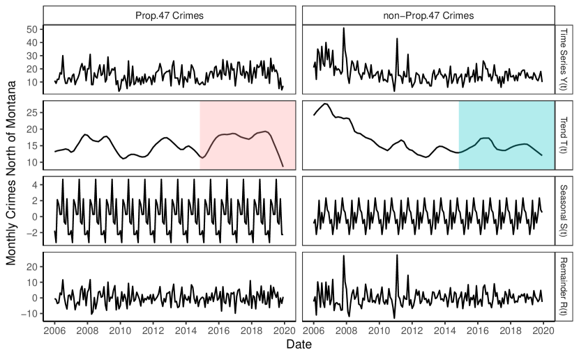
North of Montana

 Wilshire/Montana

Figure 16: STL decomposition for 2006-2019 monthly crimes in the North of Montana and Wilshire/Montana neighborhoods. Prop. 47 (non-Prop. 47) crimes are to the left (right).

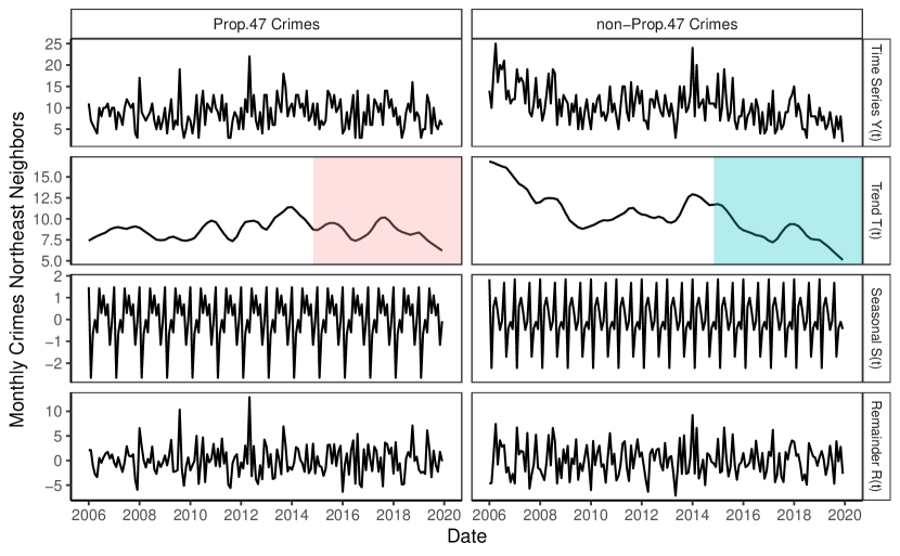
Northeast Neighbors

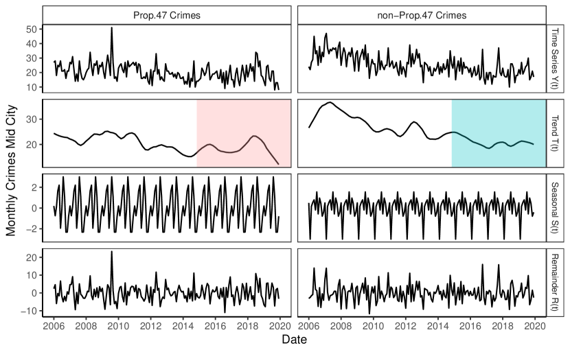
 Mid City

Figure 17: STL decomposition for 2006-2019 monthly crimes in the Northeast Neighbors and Mid City neighborhoods. Prop. 47 (non-Prop. 47) crimes are to the left (right).

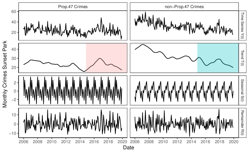
Sunset Park

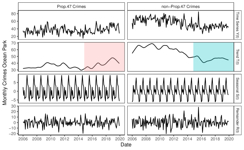
 Ocean Park

Figure 19: STL decomposition for monthly crimes from 2006 to 2019 in the Sunset Park and Ocean Park neighborhoods. Prop. 47 (non-Prop. 47) crimes are to the left (right).

References

- Adair, (1984) Adair, J. G. (1984). The Hawthorn effect: A reconsideration of the methodological artifact. Journal of Applied Psychology, 69:334–345.
- Ballotpedia, (2014) Ballotpedia (2014). California Proposition 47, Reduced Penalties for Some Crimes Initiative. https://ballotpedia.org/California_Proposition_47,_Reduced_Penalties_for_Some_Crimes_Initiative_(2014). Accessed 01 Apr 2020.
- Bang et al., (2006) Bang, H., Mazumdar, M., and Spence, J. D. (2006). Tutorial in Biostatistics: Analyzing associations between total plasma homocysteine and B vitamins using optimal categorization and segmented regression. Neuroepidemiology, 27:188–200.
- Bartos and Kubrin, (2018) Bartos, B. J. and Kubrin, C. E. (2018). Can we downsize our prisons and jails without compromising public safety? Findings from California’s Prop. 47. Criminology Public Policy, 17:693–715.
- Bird et al., (2018) Bird, M., Lofstrom, M., Martin, B., Raphael, S., Nguyen, V., and Goss, J. (2018). The impact of Proposition 47 on crime and recidivism. Technical report, Public Policy Institute of California.
- Bird et al., (2016) Bird, M., Tafoya, S., Grattet, R., and Nguyen, V. (2016). The impact of Proposition 47 on crime and recidivism. Technical report, Public Policy Institute of California.
- Block and Block, (2000) Block, R. and Block, C. (2000). The Bronx and Chicago: Street robbery in the environs of rapid transit stations. In Goldsmith, V., McGuire, P. G., Mollenkopf, J. H., and Ross, T. A., editors, Analyzing crime patterns: Frontiers of practice, volume 65, pages 137–152. Thousand Oaks: Sage Publications.
- Brantingham and Brantingham, (1993) Brantingham, P. J. and Brantingham, P. L. (1993). Nodes, path, and edges: Considerations on the complexity of crime and the physical environment. Journal of Environmental Criminology, 65:3–28.
- Brantingham et al., (1991) Brantingham, P. J., Brantingham, P. L., and Wong, P. S. (1991). How public transit feeds private crime: Notes on the Vancouver ‘Sky Train’ experience. Journal of Environmental Criminology, 2:91–94.
- Brantingham and Brantingham, (1995) Brantingham, P. L. and Brantingham, P. J. (1995). Criminality of place: Crime generators and crime attractors. European Journal on Criminal Policy and Research, 3:1–26.
- Cagle, (2018) Cagle, K. (2018). Most Read of 2018: Santa Monica sees 12 percent spike in crime. https://www.smdp.com/most-read-of-2018-santa-monica-sees-12-percent-spike-in-crime/171752. Retrieved from the Santa Monica Daily Press; accessed 01 Apr 2020.
- Casuso, (2018) Casuso, J. (2018). Suspects in Santa Monica’s most violent crimes were repeat offenders. https://www.surfsantamonica.com/ssm_site/the_lookout/news/News-2018/March-2018/03_14_2018_Suspects_in_Santa_Monicas_Most_Violent_Crimes_Were_Repeat_Offenders.html. Retrieved from Surf Santa Monica; accessed 01 Apr 2020.
- Catanzaro, (2019) Catanzaro, S. (2019). Santa Monica sees nearly 9 percent spike in Part 1 crimes. https://smmirror.com/2019/02/crime-update/. Retrieved from the Santa Monica Mirror, accessed 01 Apr 2020.
- Cervantes, (2016) Cervantes, N. (2016). Theft and similar crimes jump more than 50 percent near Santa Monica Expo Line. https://www.surfsantamonica.com/ssm_site/the_lookout/news/News-2016/December-2016/12_06_2016_Theft_and_Similar_Crimes_Jump_More_50_Percent_Near_Santa_Monica_Expo_Line.html. Retrieved from Surf Santa Monica; accessed 01 Apr 2019.
- Chen and Gupta, (2011) Chen, J. and Gupta, A. K. (2011). Parametric statistical change point analysis. Birkhäuser, Boston, MA, edition.
- Cleveland et al., (1990) Cleveland, R. B., Cleveland, W. S., McRae, J. E., and Terpenning, I. (1990). STL: A seasonal-trend decomposition procedure based on Loess. Journal of Official Statistics, 6:3–33.
- Denver Regional Transportation District, (2006) Denver Regional Transportation District (2006). Neighborhood vs. Station. Crime myths and facts. Technical report.
- Egelko, (2018) Egelko, B. (2018). Prop. 47 is linked to increase in auto thefts, study says. https://www.sfchronicle.com/crime/article/Prop-47-is-linked-to-increase-in-auto-thefts-12989137.php?psid=kOXnt. Retrieved from the San Francisco Chronicle, accessed 01 Apr 2020.
- Falk, (1952) Falk, G. (1952). The influence of the seasons on the crime rate. Journal of Criminal Law and Criminology, 43:199–213.
- Federal Bureau of Investigation, (2004) Federal Bureau of Investigation (2004). Uniform Crime Reporting Handbook. Technical report, US Department of Justice.
- Federal Bureau of Investigation, (2017) Federal Bureau of Investigation (2017). Crime in the United States, 2017. Technical report, US Department of Justice.
- Federal Reserve System, (2018) Federal Reserve System (2018). Changes in US payments fraud from 2012 to 2016: Evidence from the Federal Reserve payments study. Technical report, Board of Governors. Table B.1.A.
- Felson et al, (1996) Felson et al, M. (1996). Redesigning hell: Preventing crime and disorder at the Port Authority bus terminal. In Clarke, R. V., editor, Preventing mass transit crime. Criminal Justice Press, Monsey, NY.
- Fischer, (2018) Fischer, B. J. (2018). Proposition 47 and crime: A difference in differences analysis of incarceration rates and crime using border counties. Master’s thesis, Hunter College, City University of New York, CUNY Academic Works.
- Grattet and Bird, (2018) Grattet, R. and Bird, M. (2018). Next steps in jail and prison downsizing. Criminology and Public Policy, 17:717–726.
- Hanisee, (2018) Hanisee, M. (2018). It’s time to fix justice-reform laws. https://www.vcstar.com/story/opinion/columnists/2018/04/28/its-time-fix-justice-reform-laws/556586002/. Retrieved from the Ventura County Star; accessed 01 Apr 2020.
- Harlander, (2018) Harlander, T. (2018). Some Santa Monica residents are blaming a spike in crime on the Expo Line. https://www.lamag.com/citythinkblog/santa-monica-crime-expo-line/. Retrieved from The Los Angeles Magazine; accessed 01 Apr 2020.
- Holland and Smith, (2017) Holland, G. and Smith, D. (2017). L.a. county homelessness jumps a staggering 23 as need far outpaces housing, new count shows. http://www.latimes.com/local/lanow/lamelnhomelesscount20170530story.html. Retrieved from the Los Angeles Times; accessed 01 Apr 2020.
- Hunter et al., (2017) Hunter, S. B., Davis, L. M., Smart, R., and Turner, S. (2017). Impact of Proposition 47 on Los Angeles County operations and budget. Technical report, The RAND Corporation.
- Ihlanfeldt, (2003) Ihlanfeldt, K. R. (2003). Rail transit and neighborhood crime: The case of Atlanta, Georgia. Southern Economic Journal, 70:273–294.
- Kamel, (2012) Kamel, N. (2012). The actualization of neoliberal space and the loss of housing affordability in santa monica, california. Geoforum, 43:453–463.
- Keep California Safe, (2020) Keep California Safe (2020). Reducing crime and keeping California safe act of 2020. https://keepcalsafe.org/. Accessed 01 Apr 2020.
- Killick and Eckley, (2014) Killick, R. and Eckley, I. A. (2014). Changepoint: An R package for changepoint analysis. Journal of Statistical Software, 58:1–19.
- Killick et al., (2016) Killick, R., Haynes, K., and Eckley, I. A. (2016). Changepoint: An R package for changepoint analysis. R-package Version 2.2.2.
- La Vigne, (1996) La Vigne, N. G. (1996). Safe transport: Security by design on the Washington Metro. In Clarke, R. V., editor, Preventing mass transit crime. Criminal Justice Press, Monsey, NY.
- Langton et al., (2012) Langton, L., Berzofsky, M., Krebs, C., and Smiley-McDonald, H. (2012). Victimizations not reported to the police, 2006–2010. Technical report, US Department of Justice, Bureau of Justice Statistics.
- Lauritsen and White, (2014) Lauritsen, J. L. and White, N. (2014). Seasonal patterns in criminal victimization trends. Technical report, U.S. Department of Justice, Bureau of Justice Statistics.
- Lehner, (2016) Lehner, R. M. (2016). Effects of the Safe Neighborhoods and Schools Act (Proposition 47) on Crime Rates in California. Technical report, California Police Chiefs Association.
- Levine et al., (1986) Levine, N., Wachs, M., and Shirazi, E. (1986). Crime at bus stops: A study of environmental factors. Journal of Architectural and Planning Research, 3:339–361.
- Loukaitou-Sideris, (1999) Loukaitou-Sideris, A. (1999). Hot spots of bus stop crime: The importance of environmental attributes. Journal of the American Planning Association, 65:395–411.
- Loukaitou-Sideris et al., (2002) Loukaitou-Sideris, A., Liggett, R., and Hiseki, H. (2002). The geography of transit crime: Documentation and evaluation of crime incidence on and around the Green line stations in Los Angeles. Journal of Planning Education and Research, 22:135–151.
- Males, (2016) Males, M. (2016). Is Proposition 47 to blame for California’s 2015 increase in urban crime? Technical report, Center on Juvenile and Criminal Justice.
- McDowall et al., (2012) McDowall, D., Loftin, C., and Pate, M. (2012). The influence of the seasons on the crime rate. Seasonal cycles in crime, and their variability, 28:389–410.
- Meier et al., (2019) Meier, A., Cho, H., and Kirch, C. (2019). Mosum: Moving sum based procedures for changes in the mean. R-package Version 1.2.1.
- Mooney et al., (2018) Mooney, A. C., Giannella, E., Glymour, M. M., Neilands, T. B., Morris, M. D., Tulsky, J., and Sudhinaraset, M. (2018). Racial/ethnic disparities in arrests for drug possession after California Proposition 47, 2011-2016. American Journal of Public Health, Criminal Justice, 108:987–993.
- Mooney et al., (2019) Mooney, A. C., Neilands, T. B., Giannella, E., Morris, M. D., Tulsky, J., and Glymour, M. M. (2019). Effects of a voter initiative on disparities in punishment severity for drug offenses across California counties. Social Science and Medicine, 230:9–19.
- Muggeo, (2008) Muggeo, V. M. (2008). Segmented: An R package to fit regression models with broken-line relationships. R News, 8:20–25.
- Newman and Scott, (2012) Newman, W. J. and Scott, C. L. (2012). Brown v. Plata: prison overcrowding in california. Journal of the American Academy of Psychiatry and the Law, 40:547–52.
- Neworth, (2017) Neworth, J. (2017). Has the Expo turned into the Crime Train? http://smdp.com/has-the-expo-turned-into-the-crime-train/163250. Retrieved from the Santa Monica Daily Press; accessed 01 Apr 2020.
- Owen and Mobley, (2012) Owen, B. and Mobley, A. (2012). Realignment in California: Policy and Research implication. Western Criminology Review, 13:46–52.
- Page, (1954) Page, E. S. (1954). Continuous inspection schemes. Biometrika, 44:248–252.
- Page, (1957) Page, E. S. (1957). On problems in which a change in a parameter occurs at an unknown point. Biometrika, 41:100–115.
- (53) Pauker, M. (2019a). Crime rate drops in first four months of the year. https://www.smdp.com/crime-rate-drops/175510. Retrieved from the Santa Monica Daily Press; accessed 01 Apr 2020.
- (54) Pauker, M. (2019b). Serious crime falls 16 in Santa Monica. https://www.smdp.com/serious-crime-falls-16-in-santa-monica/185455. Retrieved from the Santa Monica Daily Press; accessed 01 Apr 2020.
- (55) Pauker, M. (2019c). Serious crime in Santa Monica rises 8.8 percent. https://www.smdp.com/serious-crime-in-santa-monica-rises-8-8-percent/172447. Retrieved from the Santa Monica Daily Press; accessed 01 Apr 2020.
- Poister, (1996) Poister, T. H. (1996). Transit-related crime in suburban areas. Journal of Urban Affairs, 18:63–75.
- R Core Team, (2018) R Core Team (2018). R: A language and environment for statistical computing. R Foundation for Statistical Computing, Vienna, Austria.
- Renaud, (2019) Renaud, C. (2019). Santa Monica crime update from Police Chief Cynthia Renaud. Seascape, 13:7–9.
- Residocracy Santa Monica, (2020) Residocracy Santa Monica (2020). https://www.facebook.com/groups/616567778411018. Facebook Page; accessed 01 Apr 2020.
- Roethlisberger and Dickson, (1939) Roethlisberger, F. J. and Dickson, W. J. (1939). Management and the worker. Harvard Univ. Press.
- Romano, (2015) Romano, M. (2015). Proposition 47 Progress report: Year one implementation. Technical report, Stanford Justice Advocacy Project.
- San Diego Association of Governments, (2009) San Diego Association of Governments (2009). Understanding transit’s impact on public safety. Technical report.
- Santa Monica Crime Watch, (2020) Santa Monica Crime Watch (2020). https://www.facebook.com/groups/santamonicacrime. Facebook Page; accessed 01 Apr 2020.
- Santa Monica Now, (2020) Santa Monica Now (2020). https://www.facebook.com/groups/SantaMonicaNow. Facebook Page; accessed 01 Apr 2020.
- Santa Monica Police Department, (2020) Santa Monica Police Department (2020). Santa Monica Open Data, Police Incidents. https://data.smgov.net/Public-Safety/Police-Incidents/kn6p-4y74/data. Accessed 01 Apr 2020.
- Santa Monica Problems, (2020) Santa Monica Problems (2020). https://www.instagram.com/santamonicaproblems/. Instagram Page; accessed 01 Apr 2020.
- Satterthwaite, (1946) Satterthwaite, F. E. (1946). An approximate distribution of estimates of variance components. Biometrics Bulletin, 2:110–114.
- Sheriff’s Department, (2018) Sheriff’s Department (2018). Proposition 47 Report. Technical report, Los Angeles County.
- Taylor, (2016) Taylor, M. (2016). The 2016-17 Budget: Fiscal impacts of Proposition 47. Technical report, Public Policy Institute of California.
- Thrasher and Schnell, (1974) Thrasher, E. J. and Schnell, J. B. (1974). Scope of crime and vandalism on urban transit systems. Transportation Research Record, 487:34–45.
- Walck, (2007) Walck, C. (2007). Hand-book on statistical distributions for experimentalists. Technical report, Particle Physics group Fysikum University of Stockholm.
- Weisberg, (2019) Weisberg, R. (2019). The Wild West of sentencing reform: Lessons from California. Crime and Justice, 48:35–77.
- Welch, (1947) Welch, B. L. (1947). The generalization of ”student’s” problem when several different population variances are involved. Biometrika, 34:28–35.
- World Population Review, (2018) World Population Review (2018). http://worldpopulationreview.com/us-cities/santa-monica-population/. Retrieved from the World Population Review website; accessed 01 Apr 2020.