An entropy stable high-order discontinuous Galerkin spectral element method for the Baer-Nunziato two-phase flow model

Abstract

In this work we propose a high-order discretization of the Baer-Nunziato two-phase flow model (Baer and Nunziato, Int. J. Multiphase Flow, 12 (1986), pp. 861-889) with closures for interface velocity and pressure adapted to the treatment of discontinuous solutions, and stiffened gas equations of states. We use the discontinuous Galerkin spectral element method (DGSEM), based on collocation of quadrature and interpolation points (Kopriva and Gassner, J. Sci. Comput., 44 (2010), pp. 136-155). The DGSEM uses summation-by-parts (SBP) operators in the numerical quadrature for approximating the integrals over discretization elements (Carpenter et al., SIAM J. Sci. Comput., 36 (2014), pp. B835-B867; Gassner et al., J. Comput. Phys., 327 (2016), pp. 39-66). Here, we build upon the framework provided in (F. Renac, J. Comput. Phys., 382 (2019), pp. 1-36) for nonconservative hyperbolic systems to modify the integration over cell elements using the SBP operators and replace the physical fluxes with entropy conservative fluctuation fluxes from Castro et al. (SIAM J. Numer. Anal., 51 (2013), pp. 1371-1391), while we derive entropy stable fluxes applied at interfaces. This allows to establish a semi-discrete inequality for the cell-averaged physical entropy, while being high-order accurate. The design of the numerical fluxes also formally preserves the kinetic energy at the semi-discrete level. High-order integration in time is performed using strong stability-preserving Runge-Kutta schemes and we propose conditions on the numerical parameters for the positivity of the cell-averaged void fraction and partial densities. The positivity of the cell-averaged solution is extended to nodal values by the use of an a posteriori limiter. The high-order accuracy, nonlinear stability, and robustness of the present scheme are assessed through several numerical experiments in one and two space dimensions.

Keywords. Compressible two-phase flows, Baer-Nunziato model, entropy stable scheme, discontinuous Galerkin method, summation-by-parts

AMS subject classifications. 65M12, 65M70, 76T10

1 Introduction

Compressible two-phase flow models find extensive applications in engineering and physics. For instance, in the aerospace industry, they are used to model the flow of a mixture of liquid kerosene and air through the combustion chamber of jet engines, whereas, in the oil and gas industry they are used to model and simulate the extraction of oil through pipelines. Elsewhere, in the nuclear industry these models are used to study and simulate the flow inside a pressurized water reactor. One of the models commonly employed for the study of compressible two-phase flows is the Baer-Nunziato model [5], which was originally proposed to describe the flow of a mixture of energetic granular material embedded in gaseous combustion product. This was later modified and adapted to the study of mixture of gas and liquid in [57, 17, 20, 27]. In general, the model is a two-velocity, two-pressure, two-temperature system that describes two-phase flows in complete disequilibrium with respect to the chemical, mechanical, thermal, and thermodynamic processes. The interaction between the phases are governed by the presence of nonconservative products and zeroth order relaxation source terms. In this work we will neglect the source terms and limit ourselves to the convective part of the model. However, the homogeneous model under consideration is fairly general using closure laws for the interface velocity and pressure [17, 27] as well as stiffened gas equations of states (EOS) relevant for flows with both liquid and gas phases.

The homogeneous Baer-Nunziato model is a system of first order, nonlinear, nonconservative partial differential equations. The system is hyperbolic and may become weakly hyperbolic and even resonant. Hyperbolic systems may generate discontinuous solutions in finite time even for smooth initial data, however, in the case of nonconservative systems, the definition of the nonconservative product is not unique at discontinuities in the classical sense of distributions and leads to an ambiguity in the value of the product. Following the notion of the Rankine-Hugoniot conditions from conservation laws, the jump conditions for nonconservative systems may be generalized and may be either based on the choice of Lipschitz paths connecting separate states around discontinuities [19], or based on the kinetic relations derived from the physical entropy [6]. Furthermore, uniqueness of the solution requires satisfying a nonlinear stability condition, for a given convex entropy function, called the entropy condition.

Numerical schemes that approximate hyperbolic systems should ideally recover admissible solutions by satisfying a discrete entropy condition [47, 34]. This property of the numerical scheme is known as entropy stability. In the case of conservation laws, Tadmor [61] provided the framework for entropy conservative and entropy stable numerical fluxes which allow for either conservation or dissipation of entropy in space by three-point finite volume schemes. This was extended to nonconservative systems in [50, 10] by the use of fluctuation fluxes and the theory of connecting paths [19]. However, path-consistent schemes do not always converge to the right admissible solutions as the solutions are dependent on the choice of path which defines the jump relation and hence the viscous profile used to attain entropy stability [2, 12, 14]. Entropy stable schemes using fluctuation fluxes to discretize nonconservative hyperbolic systems can be found in [36, 9, 53] and we refer to [48] for a review.

High-order accuracy of the numerical scheme is another exceedingly desirable quality that one seeks. The path-consistent framework can easily be adapted to high-order schemes by using reconstruction operators [11], central schemes [13], discontinuous Galerkin (DG) methods [56, 26, 16], or ADER methods [22, 21]. Among these the DG methods have gained substantial popularity over the years. The semi-discrete form of the DG method is proven to satisfy an entropy inequality for square entropy functions in scalar conservation laws [42], which was extended to symmetric systems in [37].

In [30], Gassner and coauthors have proposed an entropy stable high-order scheme for the compressible Euler equations using the discontinuous Galerkin spectral elements method (DGSEM), which was extended to general conservation laws in [16]. They used the general framework for conservative elementwise flux differencing schemes [24] satisfying a semi-discrete entropy inequality for the cell-averaged entropy. The DGSEM is based on collocation of quadrature nodes with interpolation points using the Gauss-Lobatto quadrature rules [45]. The scheme was shown to satisfy the summation-by-parts (SBP) property [28] for the discrete operators which allows to take into account the numerical quadrature that approximates integrals compared to other techniques that require their exact evaluation [42, 35, 36]. Such a form of the nodal DG method has found tremendous use in the development of entropy stable high-order schemes for the compressible Euler equations [30, 16] and multicomponent Euler equations [54], the shallow water equations [64], the magnetohydrodynamic (MHD) equations [49, 8, 65] and gradient flows [60]. In the case of nonconservative systems, a semi-discrete framework was proposed in [53] based on the DGSEM formulation that proves to be entropy stable and high-order accurate.

In the present work we utilize the framework from [53] and focus on the design of a high-order entropy stable scheme for the Baer-Nunziato model. This framework is here extended to systems that contain both space derivatives in divergence form and nonconservative products, which is based on a direct generalization of the frameworks of entropy stable finite volume schemes for conservation laws [61] and for nonconservative systems [10]. Such generalization has already been proposed for balance laws in [10]. This generalization allows the design of discretizations that reduce to conservative schemes using conservative numerical fluxes when the nonconservative products vanish as it is the case away from material fronts in the Baer-Nunziato model. Using this framework, we modify the integration over cell elements using the SBP operator and replace the physical fluxes with two-point entropy conservative fluxes in fluctuation form [10], while we use entropy stable fluxes at the cell interfaces [10, 53]. The entropy conservative fluxes are derived by using the entropy condition [10], and we add upwind-type dissipation as advocated in [40] to obtain the entropy stable numerical fluxes. The scheme is also kinetic energy preserving at the semi-discrete level. The present method is introduced in one space dimension for the sake of clarity and we provide details on its extension to multiple space dimensions on Cartesian meshes in the appendices. The extension of the DGSEM to quadrangles and hexahedra is direct and based on tensor products of one-dimensional basis functions and quadrature rules.

We then focus on high-order integration in time for which we rely on strong stability-preserving explicit Runge-Kutta schemes [59, 32] which are defined as convex combinations of first-order schemes and keep their properties under some condition on the time step. We analyze the properties of the fully discrete one-step scheme and derive explicit conditions on the time step and numerical parameters to maintain the positivity of the cell-averaged partial densities and a maximum principle for the cell-averaged void fraction. Positivity of the solution is then enforced at nodal values by the use of a posteriori limiters [66, 67]. Numerical tests in one and two space dimensions are finally performed to assess the properties of the present scheme.

The plan of the paper is as follows. Section 2 describes the Baer-Nunziato model and highlights its physical and mathematical properties. In section 3, we introduce the DGSEM framework and the semi-discrete scheme. The derivation of entropy conservative and entropy stable numerical fluxes are outlined in section 4. The properties of the scheme and the limiters are described in section 5. The results of the numerical experiments in one space dimension are presented in section 6, while those in two space dimensions are presented in section 7. Finally, concluding remarks on the present work are provided in section 8.

2 Baer-Nunziato model

We consider the Cauchy problem for the homogeneous Baer-Nunziato two-phase flow model in one space dimension [4, 23, 63, 3]:

$$\partial_{t}{\textbf{u}}+\partial_{x}\textbf{f}({\textbf{u}})+\textbf{c}({\textbf{u}})\partial_{x}{\textbf{u}} =0,\quad x\in\mathbb{R},t>0,$$ (1a)

$${\textbf{u}}(x,0) ={\textbf{u}}_{0}(x),\quad x\in\mathbb{R},$$ (1b)

where

$${\textbf{u}}\mathrel{\mathop{\mathchar 58\relax}}=\begin{pmatrix}\alpha_{i}\\ \alpha_{i}\rho_{i}\\ \alpha_{i}\rho_{i}u_{i}\\ \alpha_{i}\rho_{i}E_{i}\end{pmatrix},\quad\textbf{f}({\textbf{u}})\mathrel{\mathop{\mathchar 58\relax}}=\begin{pmatrix}0\\ \alpha_{i}\rho_{i}u_{i}\\ \alpha_{i}(\rho_{i}u^{2}_{i}+\mathrm{p}_{i})\\ \alpha_{i}u_{i}(\rho_{i}E_{i}+\mathrm{p}_{i})\end{pmatrix},\quad\textbf{c}({\textbf{u}})\partial_{x}{\textbf{u}}\mathrel{\mathop{\mathchar 58\relax}}=\begin{pmatrix}\mathrm{u_{I}}\\ 0\\ -\mathrm{p_{I}}\\ -\mathrm{p_{I}}\mathrm{u_{I}}\end{pmatrix}\partial_{x}\alpha_{i},\quad i=1,2.$$ (2)

The phase densities are $\rho_{i}$, the velocities are $u_{i}$, and the specific total energies are $E_{i}=e_{i}+u^{2}_{i}/2$ where $e_{i}$ is the specific internal energy and $i=1,2$ refers to the $i$th phase. The void fraction of each individual phase is denoted as $\alpha_{i}$ and we assume that both satisfy the saturation condition

$$\alpha_{1}+\alpha_{2}=1.$$ (3)

In one space dimension, the model is a system of seven equations including the evolution equations for the mass, momentum and energy of each phase, along with a transport equation for the void fraction. Note that the vector of unknowns, u, has seven components even though the abstract notation in (eq. 2) seems to indicate eight equations. This is due to the saturation condition (eq. 3) which allows the void fraction equation to be expressed in terms of either phases. The solution u belongs to the phase space

$$\Omega_{\scalebox{0.8}{$\scriptscriptstyle\rm BNM$}}=\big{\{}{\textbf{u}}\in\mathbb{R}^{7}\mathrel{\mathop{\mathchar 58\relax}}\,0<\alpha_{i}<1,\,\rho_{i}>0,\,u_{i}\in\mathbb{R},\,e_{i}>0,\,i=1,2\big{\}}.$$ (4)

Space variations of the physical quantities are governed by the flux function $\textbf{f}({\textbf{u}})\mathrel{\mathop{\mathchar 58\relax}}\Omega_{\scalebox{0.8}{$\scriptscriptstyle\rm BNM$}}\rightarrow\mathbb{R}^{7}$ and the nonconservative product $\textbf{c}({\textbf{u}})\partial_{x}{\textbf{u}}$ which couples the phases and hinders the system (eq. 1a) to be written in divergence form. Note that if $\alpha_{i}$ is uniform in space, the phases decouple into separate systems of compressible Euler equations.

The pressure of each phase $\mathrm{p}_{i}$ is related to the density and internal energy through a stiffened gas EOS:

$$\mathrm{p}_{i}(\rho_{i},e_{i})=(\gamma_{i}-1)\rho_{i}e_{i}-\gamma_{i}\mathrm{p}_{\infty,i},$$ (5)

where $\gamma_{i}=\mathrm{C_{p}}_{i}/\mathrm{C_{v}}_{i}>1$ is the ratio of specific heats of phase $i$ and $\mathrm{p}_{\infty,i}\geqslant 0$ are some constants. System (eq. 1a) is supplemented with closure laws for the interfacial velocity and pressure, $\mathrm{u_{I}}$ and $\mathrm{p_{I}}$, respectively, that govern the exchange of information at the interface of the two phases. In this work, we use definitions of the interfacial velocity and pressure based on convex combinations of the velocities and pressures of the two phases [17, 27] and adapted to the treatment of discontinuous solutions:

$$\mathrm{u_{I}} \mathrel{\mathop{\mathchar 58\relax}}=\beta u_{1}+(1-\beta)u_{2},$$ (6a)

$$\mathrm{p_{I}} \mathrel{\mathop{\mathchar 58\relax}}=\mu\mathrm{p}_{1}+(1-\mu)\mathrm{p}_{2},$$ (6b)

where the convex weights are

$$\beta=\frac{\chi\alpha_{1}\rho_{1}}{\chi\alpha_{1}\rho_{1}+(1-\chi)\alpha_{2}\rho_{2}},\quad\mu=\frac{(1-\beta)T_{2}}{\beta T_{1}+(1-\beta)T_{2}},\quad\chi\in\{0,\tfrac{1}{2},1\},$$ (7)

and $T_{i}$ denotes the temperature of the $i$th phase.

Under this particular choice for the closures (eq. 6) and (eq. 7), the interfacial velocity $\mathrm{u_{I}}$ corresponds to an eigenvalue for (eq. 1) associated to a linearly degenerate (LD) characteristic field which allows to close the jump relation across material interfaces that are associated to the nonconservative terms in (eq. 1a). The possible choices for $\chi$ in (eq. 7) are the ones that allow to obtain a conservative equation for the physical entropy for smooth solutions. Physical systems such as the Baer-Nunziato model are indeed naturally equipped with a physical entropy function. The phasic entropies read

$$s_{i}(\rho_{i},\theta_{i})=-\mathrm{C_{v}}_{i}\big{(}\ln\theta_{i}+(\gamma_{i}-1)\ln\rho_{i}\big{)},\quad i=1,2,$$ (8)

with $\theta_{i}=\tfrac{1}{T_{i}}$ the inverse of temperature, and obey the second law of thermodynamics. Smooth solutions of (eq. 1) satisfy

$$\partial_{t}\sum^{2}_{i=1}\alpha_{i}\rho_{i}s_{i}+\partial_{x}\sum^{2}_{i=1}\alpha_{i}\rho_{i}s_{i}u_{i}=\sum^{2}_{i=1}(\mathrm{p_{I}}-\mathrm{p}_{i})(\mathrm{u_{I}}-u_{i})\theta_{i}\partial_{x}\alpha_{i},$$ (9)

which indeed vanishes for the closure of interfacial quantities (eq. 6) and (eq. 7):

$$\sum^{2}_{i=1}(\mathrm{p_{I}}-\mathrm{p}_{i})(\mathrm{u_{I}}-u_{i})\theta_{i}\partial_{x}\alpha_{i}=0.$$ (10)

In the case of non-smooth solutions, such as shocks, admissible weak solutions must satisfy a nonlinear stability condition for the convex entropy function $\eta({\textbf{u}})\mathrel{\mathop{\mathchar 58\relax}}=-\sum^{2}_{i=1}\alpha_{i}\rho_{i}s_{i}$ and entropy flux $q({\textbf{u}})\mathrel{\mathop{\mathchar 58\relax}}=-\sum^{2}_{i=1}\alpha_{i}u_{i}\rho_{i}s_{i}$:

$$\partial_{t}\eta({\textbf{u}})+\partial_{x}q({\textbf{u}})\leqslant 0.$$ (11)

System (eq. 1a) can also be written in quasi-linear form as

$$\partial_{t}{\textbf{u}}+\textbf{A}({\textbf{u}})\partial_{x}{\textbf{u}}=0,\quad x\in\mathbb{R},t>0,$$ (12)

where $\textbf{A}\mathrel{\mathop{\mathchar 58\relax}}\Omega_{\scalebox{0.8}{$\scriptscriptstyle\rm BNM$}}\ni{\textbf{u}}\mapsto\textbf{A}({\textbf{u}})=\textbf{f}^{\prime}({\textbf{u}})+\textbf{c}({\textbf{u}})\in\mathbb{R}^{7\times 7}$ is a matrix-valued function for smooth solutions of (eq. 1). The system (eq. 12) is hyperbolic over the phase space (eq. 4) and A(u) admits real eigenvalues

$$\lambda_{1}({\textbf{u}})=u_{1}-c_{1},\;\lambda_{2}({\textbf{u}})=u_{2}-c_{2},\;\lambda_{3}({\textbf{u}})=u_{1},\;\lambda_{4}({\textbf{u}})=\mathrm{u_{I}},\;\lambda_{5}({\textbf{u}})=u_{2},\;\lambda_{6}({\textbf{u}})=u_{1}+c_{1},\;\lambda_{7}({\textbf{u}})=u_{2}+c_{2},$$ (13)

associated to linearly independent eigenvectors. Here $c_{i}(\rho_{i},e_{i})^{2}=\gamma_{i}(\gamma_{i}-1)(\rho_{i}e_{i}-p_{\infty,i})/\rho_{i}$ is the speed of sound for the EOS (eq. 5). Observe, in (eq. 13), that $\lambda_{3},\lambda_{4}$ and $\lambda_{5}$ are associated to LD fields, whereas the others ones, $\lambda_{1},\lambda_{2},\lambda_{6}$ and $\lambda_{7}$, are associated to genuinely nonlinear (GNL) fields. Note that (eq. 12) is only weakly hyperbolic when $\mathrm{u_{I}}$ is equal to one transport velocity, $u_{1}$ or $u_{2}$, for $\chi=1$ or $0$ in (eq. 7). In this work we assume that (eq. 12) is hyperbolic and well-posed and exclude resonance phenomena [18]:

$$\alpha_{i}\neq 0,\quad\mathrm{u_{I}}\neq u_{i}\pm c_{i},\quad i=1,2.$$ (14)

When resonance occurs, the system turns degenerate as the right eigenvectors no longer span the whole phase space (eq. 4).

During the remaining course of this work we will be interested in discretizing the initial value problem (eq. 1). We will discretize the system in space using the DGSEM framework from [53] and propose numerical fluxes that maintain the nonlinear stability condition (eq. 11) at the semi-discrete level in addition to several other properties.

3 Space discretization with the DGSEM

We discretize the physical domain using a grid $\Omega_{h}\mathrel{\mathop{\mathchar 58\relax}}=\cup_{j\in\mathbb{Z}}\kappa_{j}$ containing cells $\kappa_{j}=[x_{j-\frac{1}{2}},x_{j+\frac{1}{2}}]$, $x_{j+\frac{1}{2}}=jh$ with cell size $h>0$, see Figure 1. Here the mesh is assumed to be uniform without loss of generality.

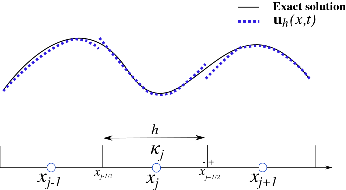
Figure 1: A one-dimensional representation of the mesh with cells $\kappa_{j}$ of size $h$. The left and right interfaces of cell $\kappa_{j}$ are at $x_{j\mp\frac{1}{2}}$, and representation of the left and right traces at $x_{j+\frac{1}{2}}$.

3.1 Numerical solution

We look for approximate solutions in the function space of piecewise polynomials

$$\mathcal{V}^{p}_{h}=\big{\{}v_{h}\in L^{2}(\Omega_{h})\mathrel{\mathop{\mathchar 58\relax}}v_{h}|_{\kappa_{j}}\in\mathcal{P}_{p}(\kappa_{j}),\kappa_{j}\in\Omega_{h}\big{\}},$$ (15)

where $\mathcal{P}_{p}(\kappa_{j})$ denotes the space of polynomials of degree at most $p$ in the element $\kappa_{j}$. The approximate solution to (eq. 1) is sought as

$${\textbf{u}}_{h}(x,t)=\sum^{p}_{k=0}\phi^{k}_{j}(x)\textbf{U}^{k}_{j}(t)\quad\forall x\in\kappa_{j},\kappa_{j}\in\Omega_{h},t>0,$$ (16)

where the subset $(\phi^{0}_{j},...,\phi^{p}_{j})$ constitutes a basis of $\mathcal{V}^{p}_{h}$ restricted onto $\kappa_{j}$ and $\textbf{U}^{0\leqslant k\leqslant p}_{j}$ are the associated degrees of freedom (DOFs). Here we use the Lagrange interpolation polynomials $\ell_{0\leqslant k\leqslant p}$ associated to the Gauss-Lobatto nodes over the reference element $I=[-1,1]$: $-1=s_{0}<s_{1}<\cdots<s_{p}=1$. The basis functions thus satisfy the relation

$$\ell_{k}(s_{l})=\delta_{kl},\quad 0\leqslant k,l\leqslant p,$$ (17)

where $\delta_{kl}$ is the Kronecker symbol. The basis functions with support in a given element $\kappa_{j}$ are written as $\phi^{k}_{j}(x)=\ell_{k}(\sigma_{j}(x))$, where $\sigma_{j}(x)=2(x-x_{j})/h$ and $x_{j}=(x_{j+\frac{1}{2}}+x_{j-\frac{1}{2}})/2$ denotes the center of the element.

The DOFs thus correspond to the point values of the solution: given $0\leqslant k\leqslant p$, $j\in\mathbb{Z}$, and $t\geqslant 0$, we have ${\textbf{u}}_{h}(x^{k}_{j},t)=\textbf{U}^{k}_{j}(t)$ for $x^{k}_{j}=x_{j}+s_{k}h/2$. Likewise, the left and right traces of the solution at the element interfaces are ${\textbf{u}}_{h}(x^{-}_{j+1/2},t)=\textbf{U}^{p}_{j}(t)$ and ${\textbf{u}}_{h}(x^{+}_{j-1/2},t)=\textbf{U}^{0}_{j}(t)$, respectively. The integrals over the elements are approximated using the Gauss-Lobatto quadrature rule, where the points are collocated with the interpolation points of the numerical solution:

$$\int_{\kappa_{j}}f(x)dx\approx\frac{h}{2}\sum^{p}_{l=0}\omega_{l}f(x^{l}_{j}),$$ (18)

where $\omega_{l}>0$, with $\sum^{p}_{l=0}\omega_{l}=2$, are the quadrature weights and $x^{l}_{j}$ the quadrature points. This allows to define the discrete inner product in the element $\kappa_{j}$ as

$$\langle f,g\rangle^{p}_{j}\mathrel{\mathop{\mathchar 58\relax}}=\frac{h}{2}\sum^{p}_{l=0}\omega_{l}f(x^{l}_{j})g(x^{l}_{j}).$$ (19)

We also introduce the discrete difference matrix

$$D_{kl}=\ell^{\prime}_{l}(s_{k})=\frac{h}{2}d_{x}\phi^{l}_{j}(x^{k}_{j}),\quad 0\leqslant k,l\leqslant p.$$ (20)

This operator satisfies the summation-by-parts property, as noticed in [45],

$$\omega_{k}D_{kl}+\omega_{l}D_{lk}=\delta_{kp}\delta_{lp}-\delta_{k0}\delta_{l0}\quad\forall 0\leqslant k,l\leqslant p,$$ (21)

which is the discrete analogue of the following integration-by-parts

$$\int_{\kappa_{j}}\phi^{k}_{j}(x)d_{x}\phi^{l}_{j}(x)dx+\int_{\kappa_{j}}d_{x}\phi^{k}_{j}(x)\phi^{l}_{j}(x)dx=\big{[}\phi^{k}_{j}(x)\phi^{l}_{j}(x)\big{]}^{x^{-}_{j+1/2}}_{x^{+}_{j-1/2}},$$ (22)

since the Gauss-Lobatto quadrature rule is exact for polynomial integrands up to degree $2p-1$. Furthermore the property $\sum^{p}_{l=0}\ell_{l}\equiv 1$ implies

$$\sum^{p}_{l=0}D_{kl}=0\quad\forall 0\leqslant k\leqslant p.$$ (23)

3.2 Semi-discrete form

The semi-discrete DGSEM formulation of (eq. 1a), see [56, 25, 53], reads: find ${\textbf{u}}_{h}$ in $(\mathcal{V}^{p}_{h})^{7}$ such that

$$\int_{\Omega_{h}}v_{h}\partial_{t}{\textbf{u}}_{h}dx+\int_{\Omega_{h}}v_{h}\big{(}\partial_{x}{\bf f}({\textbf{u}}_{h})+\textbf{c}({\textbf{u}}_{h})\partial_{x}{\textbf{u}}_{h}\big{)}dx +\sum_{j\in\mathbb{Z}}v_{h}\big{(}x^{-}_{j+\frac{1}{2}}\big{)}{\textbf{D}}^{-}\big{(}\textbf{U}^{p}_{j}(t),\textbf{U}^{0}_{j+1}(t)\big{)}$$ (24)

$$+\sum_{j\in\mathbb{Z}}v_{h}\big{(}x^{+}_{j-\frac{1}{2}}\big{)}{\textbf{D}}^{+}\big{(}\textbf{U}^{p}_{j-1}(t),\textbf{U}^{0}_{j}(t)\big{)}=0\quad\forall v_{h}\in\mathcal{V}^{p}_{h},t>0,$$

where ${\textbf{D}}^{\pm}(\cdot,\cdot)$ are the numerical fluxes at the interfaces in fluctuation form which will be defined below.

Upon substituting $v_{h}$ for the Lagrange interpolation polynomials $\phi^{k}_{j}(x)=\ell_{k}(\sigma_{j}(x))$, defined by (eq. 17), and using the quadrature rule (eq. 18) to approximate the volume integrals, (eq. 24) becomes

$$\frac{\omega_{k}h}{2}\frac{d\textbf{U}^{k}_{j}}{dt}+\omega_{k}\sum^{p}_{l=0}D_{kl}\big{(}\textbf{f}(\textbf{U}^{l}_{j})+\textbf{c}(\textbf{U}^{k}_{j})\textbf{U}^{l}_{j}\big{)}+\delta_{kp}{\textbf{D}}^{-}(\textbf{U}^{p}_{j},\textbf{U}^{0}_{j+1})+\delta_{k0}{\textbf{D}}^{+}(\textbf{U}^{p}_{j-1},\textbf{U}^{0}_{j})=0\quad\forall j\in\mathbb{Z},0\leqslant k\leqslant p,$$ (25)

along with the projection of the initial condition (eq. 1b) on the function space:

$$\textbf{U}^{k}_{j}(0)={\textbf{u}}_{0}(x^{k}_{j})\quad\forall j\in\mathbb{Z},0\leqslant k\leqslant p.$$ (26)

3.3 Numerical fluxes

We rely on numerical fluxes in fluctuation form [50] that satisfy the properties of entropy conservation and entropy stability for the semi-discrete form (eq. 25). Here we recall their definition from [10].

Definition 3.1.

Let ${{\textbf{D}}}^{\pm}_{ec}$ be Lipschitz continuous and consistent numerical fluxes in fluctuation form, ${\textbf{D}}^{\pm}_{ec}({\textbf{u}},{\textbf{u}})=0$ for all u in $\Omega_{\scalebox{0.8}{$\scriptscriptstyle\rm BNM$}}$, and $(\eta,q)$ be an entropy-entropy flux pair for (eq. 1a), then ${{\textbf{D}}}^{\pm}_{ec}$ are said to be entropy conservative if they satisfy the following relation:

$${\textbf{v}}({\textbf{u}}^{-})^{\top}{\textbf{D}}^{-}_{ec}({\textbf{u}}^{-},{\textbf{u}}^{+})+{\textbf{v}}({\textbf{u}}^{+})^{\top}{\textbf{D}}^{+}_{ec}({\textbf{u}}^{-},{\textbf{u}}^{+})=q({\textbf{u}}^{+})-q({\textbf{u}}^{-})\quad\forall{\textbf{u}}^{\pm}\in\Omega_{\scalebox{0.8}{$\scriptscriptstyle\rm BNM$}},$$ (27)

where ${\textbf{v}}({\textbf{u}}^{\pm})\mathrel{\mathop{\mathchar 58\relax}}=\eta^{\prime}({\textbf{u}}^{\pm})$ denote the entropy variables.

In this work we look for entropy conservative fluxes with the following form

$${\textbf{D}}^{-}_{ec}({\textbf{u}}^{-},{\textbf{u}}^{+}) =\textbf{h}({\textbf{u}}^{-},{\textbf{u}}^{+})-\textbf{f}({\textbf{u}}^{-})+{\textbf{d}}^{-}({\textbf{u}}^{-},{\textbf{u}}^{+}),$$ (28a)

$${\textbf{D}}^{+}_{ec}({\textbf{u}}^{-},{\textbf{u}}^{+}) =\textbf{f}({\textbf{u}}^{+})-\textbf{h}({\textbf{u}}^{-},{\textbf{u}}^{+})+{\textbf{d}}^{+}({\textbf{u}}^{-},{\textbf{u}}^{+}),$$ (28b)

where $\textbf{h}({\textbf{u}}^{-},{\textbf{u}}^{+})$ is a numerical flux that approximates the traces of the physical fluxes, $\textbf{f}({\textbf{u}}^{\pm})$, and $\textbf{d}^{\pm}({\textbf{u}}^{-},{\textbf{u}}^{+})$ are fluctuation fluxes for the discretization of the nonconservative term in (eq. 1a). The numerical fluxes satisfy the consistency conditions:

$${\textbf{h}}({\textbf{u}},{\textbf{u}})=\textbf{f}({\textbf{u}}),\quad\textbf{d}^{\pm}({\textbf{u}},{\textbf{u}})=0\quad\forall{\textbf{u}}\in\Omega_{\scalebox{0.8}{$\scriptscriptstyle\rm BNM$}}.$$ (29)

The condition for entropy conservation now becomes

$${\textbf{v}}({\textbf{u}}^{-})^{\top}{\bf d}^{-}({\textbf{u}}^{-},{\textbf{u}}^{+})+{\textbf{v}}({\textbf{u}}^{+})^{\top}{\bf d}^{+}({\textbf{u}}^{-},{\textbf{u}}^{+})+\llbracket{\textbf{v}}^{\top}{\bf f}-q\rrbracket=\textbf{h}({\textbf{u}}^{-},{\textbf{u}}^{+})\llbracket{\textbf{v}}\rrbracket\quad\forall{\textbf{u}}^{\pm}\in\Omega_{\scalebox{0.8}{$\scriptscriptstyle\rm BNM$}},$$ (30)

where $\llbracket a\rrbracket=a^{+}-a^{-}$ denotes the jump operator. This relation is a direct generalization of entropy conditions in [61, 10] for systems with conservative and nonconservative terms.

Furthermore, we seek entropy stable fluxes by adding dissipation to the entropy conservative fluxes as advocated in [40] for conservation laws:

$${\textbf{D}}^{\pm}({\textbf{u}}^{-},{\textbf{u}}^{+})\mathrel{\mathop{\mathchar 58\relax}}={\textbf{D}}^{\pm}_{ec}({\textbf{u}}^{-},{\textbf{u}}^{+})\pm{\textbf{D}}_{\nu}({\textbf{u}}^{-},{\textbf{u}}^{+}),$$ (31)

where ${\textbf{D}}_{\nu}({\textbf{u}}^{-},{\textbf{u}}^{+})$ is a numerical dissipation that satisfies consistency and entropy dissipation:

$${{\textbf{D}}}_{\nu}({\textbf{u}},{\textbf{u}})=0,\quad\llbracket{\textbf{v}}({\textbf{u}})\rrbracket^{\top}\textbf{D}_{\nu}({\textbf{u}}^{-},{\textbf{u}}^{+})\geqslant 0\quad\forall{\textbf{u}},{\textbf{u}}^{\pm}\in\Omega_{\scalebox{0.8}{$\scriptscriptstyle\rm BNM$}}.$$ (32)

Observe, in the semi-discrete form (eq. 25), that the discrete volume integral does not bear proper constraints towards entropy conservation or dissipation. In other words we cannot control the sign of its scalar product with the entropy variables. Therefore, we modify the volume integral and replace it with entropy conservative fluctuation fluxes, as in [53]. The semi-discrete scheme now reads

$$\frac{\omega_{k}h}{2}\frac{d\textbf{U}^{k}_{j}}{dt}+\textbf{R}^{k}_{j}({\textbf{u}}_{h})=0,$$ (33)

where

$$\textbf{R}^{k}_{j}({\textbf{u}}_{h})=\omega_{k}\sum^{p}_{l=0}D_{kl}\tilde{{\textbf{D}}}(\textbf{U}^{k}_{j},\textbf{U}^{l}_{j})+\delta_{kp}{\textbf{D}}^{-}(\textbf{U}^{p}_{j},\textbf{U}^{0}_{j+1})+\delta_{k0}{\textbf{D}}^{+}(\textbf{U}^{p}_{j-1},\textbf{U}^{0}_{j}),$$ (34)

and

$$\tilde{{\textbf{D}}}({\textbf{u}}^{-},{\textbf{u}}^{+}) \mathrel{\mathop{\mathchar 58\relax}}={\textbf{D}}^{-}_{ec}({\textbf{u}}^{-},{\textbf{u}}^{+})-{\textbf{D}}^{+}_{ec}({\textbf{u}}^{+},{\textbf{u}}^{-}),$$ (35a)

$$\overset{(\lx@cref{creftype~refnum}{Eqn: fluctuation flux})}{=}\textbf{h}({\textbf{u}}^{-},{\textbf{u}}^{+})+\textbf{h}({\textbf{u}}^{+},{\textbf{u}}^{-})+{\textbf{d}}^{-}({\textbf{u}}^{-},{\textbf{u}}^{+})-{\textbf{d}}^{+}({\textbf{u}}^{+},{\textbf{u}}^{-}).$$ (35b)

Note that in the above relation we do not require h to be symmetric as in [24, 16], but rather use the symmetrizer $\tfrac{1}{2}\big{(}\textbf{h}({\textbf{u}}^{-},{\textbf{u}}^{+})+\textbf{h}({\textbf{u}}^{+},{\textbf{u}}^{-})\big{)}$.

3.4 Properties of the semi-discrete scheme

The modification to the integrals over cell elements in (eq. 34) allows for an entropy stable numerical scheme that preserves the high-order accuracy of the scheme. Below we generalize the results from [53] to systems that contain both conservative and nonconservative terms.

Theorem 3.1.

Let ${{\textbf{D}}}^{\pm}$ be consistent and entropy stable fluctuation fluxes (eq. 31) and (eq. 32) in (eq. 34) and $\tilde{{\textbf{D}}}$ defined by (eq. 35b) with consistent and entropy conservative fluctuation fluxes (eq. 30) and (eq. 29). Then, the semi-discrete numerical scheme (eq. 33) satisfies an entropy inequality for the entropy-entropy flux pair $(\eta,q)$ in (eq. 11):

$$h\frac{d\langle\eta({\textbf{u}}_{h})\rangle_{j}}{dt}+Q({\textbf{U}}^{p}_{j},{\textbf{U}}^{0}_{j+1})-Q({\textbf{U}}^{p}_{j-1},{\textbf{U}}^{0}_{j})\leqslant 0,$$ (36)

where $\displaystyle\langle\eta({\textbf{u}}_{h})\rangle_{j}(t)=\sum^{p}_{k=0}\frac{\omega_{k}}{2}\eta\big{(}\textbf{U}^{k}_{j}(t)\big{)}$ is the cell averaged entropy and the conservative numerical entropy flux is defined by

$$Q({\textbf{u}}^{-},{\textbf{u}}^{+})=\frac{q({\textbf{u}}^{-})+q({\textbf{u}}^{+})}{2}+\frac{1}{2}{\textbf{v}}({\textbf{u}}^{-})^{\top}{\textbf{D}}^{-}({\textbf{u}}^{-},{\textbf{u}}^{+})-\frac{1}{2}{\textbf{v}}({\textbf{u}}^{+})^{\top}{\textbf{D}}^{+}({\textbf{u}}^{-},{\textbf{u}}^{+}).$$ (37)

Further assuming that ${\bf d}^{\pm}$ in (eq. 35b) have the form

$${\bf d}^{\pm}({\textbf{u}}^{-},{\textbf{u}}^{+}) =\mathcal{C}^{\pm}({\textbf{u}}^{-},{\textbf{u}}^{+})\llbracket{\textbf{u}}\rrbracket,$$ (38a)

$$\mathcal{C}({\textbf{u}}^{-},{\textbf{u}}^{+}) \mathrel{\mathop{\mathchar 58\relax}}=\mathcal{C}^{+}({\textbf{u}}^{-},{\textbf{u}}^{+})+\mathcal{C}^{-}({\textbf{u}}^{-},{\textbf{u}}^{+}),$$ (38b)

$$\mathcal{C}({\textbf{u}}^{-},{\textbf{u}}^{+})+\mathcal{C}({\textbf{u}}^{+},{\textbf{u}}^{-}) ={\textbf{c}}({\textbf{u}}^{-})+\textbf{c}({\textbf{u}}^{+}),$$ (38c)

$$\mathcal{C}({\textbf{u}},{\textbf{u}}) ={\textbf{c}}({\textbf{u}}),$$ (38d)

where $\llbracket{\textbf{u}}\rrbracket={\textbf{u}}^{+}-{\textbf{u}}^{-}$, then semi-discrete DGSEM (eq. 33) is a high-order approximation in space of smooth solutions for the nonconservative system (eq. 1a) that satisfies

$$h\frac{d\langle{\textbf{u}}_{h}\rangle_{j}}{dt}+\langle\textbf{c}({\textbf{u}}_{h}),d_{x}{\textbf{u}}_{h}\rangle^{p}_{j}+{\textbf{D}}^{-}(\textbf{U}^{p}_{j},\textbf{U}^{0}_{j+1})+{\bf f}(\textbf{U}^{p}_{j})+{\textbf{D}}^{+}(\textbf{U}^{p}_{j-1},\textbf{U}^{0}_{j})-{\bf f}(\textbf{U}^{0}_{j})=0,$$ (39)

for the cell averaged solution

$$\langle{\textbf{u}}_{h}\rangle_{j}(t)\mathrel{\mathop{\mathchar 58\relax}}=\frac{1}{h}\int_{\kappa_{j}}{\textbf{u}}_{h}(x,t)dx=\frac{1}{2}\sum^{p}_{k=0}\omega_{k}\textbf{U}^{k}_{j}(t).$$ (40)

Proof.

These results are consequences of, e.g., [16, Theorem 3.3] for the conservative terms and [53, Theorems 3.1 and 3.2] for the nonconserative ones. First, the entropy inequality has been proved in [53, Theorem 3.1] by using the definition (eq. 35a) of the volume terms together with the entropy condition (eq. 27). High-order accuracy of the discretization in the volume integral in (eq. 34) has been proved in [16, Theorem 3.3] for the conservative terms by using the symmetric flux $\tfrac{1}{2}\big{(}\textbf{h}({\textbf{u}}^{-},{\textbf{u}}^{+})+\textbf{h}({\textbf{u}}^{+},{\textbf{u}}^{-})\big{)}$ in (eq. 35b) and the SBP property (eq. 21), and in [53, Theorem 3.2] by using (eq. 38) and the SBP property. Finally, by summing (eq. 33) over $0\leqslant k\leqslant p$ and using (eq. 34) and (eq. 40) we obtain

$$h\frac{d\langle{\textbf{u}}_{h}\rangle_{j}}{dt}+\sum_{k=0}^{p}\sum^{p}_{l=0}\omega_{k}D_{kl}\tilde{{\textbf{D}}}(\textbf{U}^{k}_{j},\textbf{U}^{l}_{j})+{\textbf{D}}^{-}(\textbf{U}^{p}_{j},\textbf{U}^{0}_{j+1})+{\textbf{D}}^{+}(\textbf{U}^{p}_{j-1},\textbf{U}^{0}_{j})=0,$$

where

$$\sum_{k,l=0}^{p}\omega_{k}D_{kl}\tilde{{\textbf{D}}}(\textbf{U}^{k}_{j},\textbf{U}^{l}_{j}) \overset{(\lx@cref{creftype~refnum}{tilde Db})}{=}\sum_{k,l=0}^{p}\omega_{k}D_{kl}\big{(}{\bf h}(\textbf{U}^{k}_{j},\textbf{U}^{l}_{j})+{\bf d}^{-}(\textbf{U}^{k}_{j},\textbf{U}^{l}_{j})\big{)}+\sum_{k,l=0}^{p}\omega_{k}D_{kl}\big{(}{\bf h}(\textbf{U}^{l}_{j},\textbf{U}^{k}_{j})-{\bf d}^{+}(\textbf{U}^{l}_{j},\textbf{U}^{k}_{j})\big{)}$$

$$\overset{(\lx@cref{creftype~refnum}{eqn: SBP})}{\underset{(\lx@cref{creftype~refnum}{eq:consistency_h_d})}{=}}\sum_{k,l=0}^{p}\omega_{k}D_{kl}\big{(}{\bf h}(\textbf{U}^{k}_{j},\textbf{U}^{l}_{j})+{\bf d}^{-}(\textbf{U}^{k}_{j},\textbf{U}^{l}_{j})\big{)}-\sum_{k,l=0}^{p}\omega_{l}D_{lk}\big{(}{\bf h}(\textbf{U}^{l}_{j},\textbf{U}^{k}_{j})-{\bf d}^{+}(\textbf{U}^{l}_{j},\textbf{U}^{k}_{j})\big{)}+{\bf f}({\bf U}_{j}^{p})-{\bf f}({\bf U}_{j}^{0})$$

$$\overset{(\lx@cref{creftype~refnum}{eqn: high-order approximation proof a})}{\underset{(\lx@cref{creftype~refnum}{eqn: high-order approximation proof b})}{=}}\sum_{k,l=0}^{p}\omega_{k}D_{kl}{\cal C}(\textbf{U}^{k}_{j},\textbf{U}^{l}_{j})(\textbf{U}^{l}_{j}-\textbf{U}^{k}_{j})+{\bf f}({\bf U}_{j}^{p})-{\bf f}({\bf U}_{j}^{0})$$

$$\overset{(\lx@cref{creftype~refnum}{eqn: SBP})}{\underset{(\lx@cref{creftype~refnum}{eqn: high-order approximation proof d})}{=}}\sum_{k,l=0}^{p}\omega_{k}D_{kl}{\cal C}(\textbf{U}^{k}_{j},\textbf{U}^{l}_{j})\textbf{U}^{l}_{j}+\sum_{k,l=0}^{p}\omega_{l}D_{lk}{\cal C}(\textbf{U}^{k}_{j},\textbf{U}^{l}_{j})\textbf{U}^{k}_{j}-{\bf c}({\bf U}_{j}^{p}){\bf U}_{j}^{p}+{\bf c}({\bf U}_{j}^{0}){\bf U}_{j}^{0}+{\bf f}({\bf U}_{j}^{p})-{\bf f}({\bf U}_{j}^{0})$$

$$\overset{(\lx@cref{creftype~refnum}{eqn: high-order approximation proof c})}{=}\sum_{k,l=0}^{p}\omega_{k}D_{kl}\big{(}{\bf c}(\textbf{U}^{k}_{j})+{\bf c}(\textbf{U}^{l}_{j})\big{)}\textbf{U}^{l}_{j}-{\bf c}({\bf U}_{j}^{p}){\bf U}_{j}^{p}+{\bf c}({\bf U}_{j}^{0}){\bf U}_{j}^{0}+{\bf f}({\bf U}_{j}^{p})-{\bf f}({\bf U}_{j}^{0})$$

$$\overset{(\lx@cref{creftype~refnum}{eqn: SBP})}{=}\sum_{k,l=0}^{p}\omega_{k}D_{kl}{\bf c}(\textbf{U}^{k}_{j})\textbf{U}^{l}_{j}-\sum_{k,l=0}^{p}\omega_{k}D_{kl}{\bf c}(\textbf{U}^{k}_{j})\textbf{U}^{k}_{j}+{\bf f}({\bf U}_{j}^{p})-{\bf f}({\bf U}_{j}^{0})$$

$$\overset{(\lx@cref{creftype~refnum}{eq:sum_Dkl_vanishes})}{\underset{(\lx@cref{creftype~refnum}{eq:1d_inner_product})}{=}}\langle\textbf{c}({\textbf{u}}_{h}),d_{x}{\textbf{u}}_{h}\rangle^{p}_{j}+{\bf f}({\bf U}_{j}^{p})-{\bf f}({\bf U}_{j}^{0})$$

∎

Note that (eq. 39) proves that the discretization of the fluxes ${\bf f}$ in (eq. 34) is in conservative form. In the following section we propose numerical fluxes for (eq. 12) that satisfy the assumptions in Theorem 3.1.

4 Numerical fluxes for the Baer-Nunziato model

Here we derive the numerical fluxes for the model (eq. 1a) that satisfy the entropy conservation (eq. 30) and dissipation (eq. 31) properties together with the assumptions in Theorem 3.1. An essential tool which would help in the algebraic manipulations are the Leibniz identities, which we recall here. Let $a^{+},a^{-},b^{+},b^{-},c^{+},c^{-}$ in $\mathbb{R}$ have finite values, then we have

$$\llbracket ab\rrbracket=\hskip 0.12135pt\hbox to0.0pt{\leavevmode\hbox{\set@color$a$}\hss}{\footnotesize{\hskip-0.12135pt\leavevmode\hbox{\set@color$\overline{\hbox{}}$}}}\llbracket b\rrbracket+\hskip 0.56876pt\hbox to0.0pt{\leavevmode\hbox{\set@color$b$}\hss}{\footnotesize{\hskip-0.56876pt\leavevmode\hbox{\set@color$\overline{\hbox{}}$}}}\llbracket a\rrbracket,\quad\llbracket abc\rrbracket=\hskip 0.12135pt\hbox to0.0pt{\leavevmode\hbox{\set@color$a$}\hss}{\footnotesize{\hskip-0.12135pt\leavevmode\hbox{\set@color$\overline{\hbox{}}$}}}(\hskip 0.56876pt\hbox to0.0pt{\leavevmode\hbox{\set@color$b$}\hss}{\footnotesize{\hskip-0.56876pt\leavevmode\hbox{\set@color$\overline{\hbox{}}$}}}\llbracket c\rrbracket+\hskip 0.5526pt\hbox to0.0pt{\leavevmode\hbox{\set@color$c$}\hss}{\footnotesize{\hskip-0.5526pt\leavevmode\hbox{\set@color$\overline{\hbox{}}$}}}\llbracket b\rrbracket)+\hbox to0.0pt{\hskip 1.37863pt\leavevmode\hbox{\set@color$\overline{\hbox{}}$}\hss}{\footnotesize{\leavevmode\hbox{\set@color$bc$}}}\llbracket a\rrbracket,$$ (41)

where $\hskip 0.12135pt\hbox to0.0pt{\leavevmode\hbox{\set@color$a$}\hss}{\footnotesize{\hskip-0.12135pt\leavevmode\hbox{\set@color$\overline{\hbox{}}$}}}=\displaystyle\frac{a^{+}+a^{-}}{2}$ is the arithmetic mean and $\llbracket a\rrbracket=a^{+}-a^{-}$ is the jump operator.

4.1 Entropy conservative fluxes

We begin by proposing entropy conservative numerical fluxes.

Proposition 4.1.

The numerical fluxes (eq. 28) with the following definitions are consistent and entropy conservative fluxes that satisfy the assumptions (eq. 38) of Theorem 3.1 for the Baer-Nunziato model (eq. 1a) with the EOS (eq. 5) and the interface variables (eq. 6).

$${\textbf{h}}({\textbf{u}}^{-},{\textbf{u}}^{+})\mathrel{\mathop{\mathchar 58\relax}}=\begin{pmatrix}0\\ h_{\rho_{i}}\\ h_{\rho u_{i}}\\ h_{\rho E_{i}}\end{pmatrix}-\beta_{s}\frac{\llbracket\alpha_{i}\rrbracket}{2}\begin{pmatrix}1\\ \tilde{h}_{\rho_{i}}\\ \tilde{h}_{\rho u_{i}}\\ \tilde{h}_{\rho E_{i}}\end{pmatrix},\quad{\textbf{d}}^{\pm}({\textbf{u}}^{-},{\textbf{u}}^{+})\mathrel{\mathop{\mathchar 58\relax}}=\frac{\llbracket\alpha_{i}\rrbracket}{2}\begin{pmatrix}\mathrm{u_{I}}^{\pm}\\ 0\\ -\mathrm{p_{I}}^{\pm}\\ -\mathrm{p_{I}}^{\pm}\mathrm{u_{I}}^{\pm}\end{pmatrix},$$ (42)

where

$$(h_{\rho_{i}},h_{\rho u_{i}},h_{\rho E_{i}}) =\left(\hbox to0.0pt{\hskip 0.37865pt\leavevmode\hbox{\set@color$\overline{\hbox{}}$}\hss}{\footnotesize{\leavevmode\hbox{\set@color$\alpha$}}}_{i}\hbox to0.0pt{\hskip 0.07605pt\leavevmode\hbox{\set@color$\overline{\hbox{}}$}\hss}{\footnotesize{\leavevmode\hbox{\set@color$u$}}}_{i}\hat{\rho}_{i},\;\hbox to0.0pt{\hskip 0.37865pt\leavevmode\hbox{\set@color$\overline{\hbox{}}$}\hss}{\footnotesize{\leavevmode\hbox{\set@color$\alpha$}}}_{i}\left(\hbox to0.0pt{\hskip 0.07605pt\leavevmode\hbox{\set@color$\overline{\hbox{}}$}\hss}{\footnotesize{\leavevmode\hbox{\set@color$u$}}}^{2}_{i}\hat{\rho}_{i}+\tfrac{\hbox to0.0pt{\hskip 1.94415pt\leavevmode\hbox{\set@color$\overline{\hbox{}}$}\hss}{\footnotesize{\leavevmode\hbox{\set@color$\mathrm{p}_{i}\theta_{i}$}}}}{\hskip 1.02126pt\hbox to0.0pt{\leavevmode\hbox{\set@color$\theta$}\hss}{\footnotesize{\hskip-1.02126pt\leavevmode\hbox{\set@color$\overline{\hbox{}}$}}}_{i}}\right),\;\hbox to0.0pt{\hskip 0.37865pt\leavevmode\hbox{\set@color$\overline{\hbox{}}$}\hss}{\footnotesize{\leavevmode\hbox{\set@color$\alpha$}}}_{i}\hbox to0.0pt{\hskip 0.07605pt\leavevmode\hbox{\set@color$\overline{\hbox{}}$}\hss}{\footnotesize{\leavevmode\hbox{\set@color$u$}}}_{i}\left(\hat{\rho}_{i}\left(\tfrac{\mathrm{C_{v}}_{i}}{\hat{\theta}_{i}}+\tfrac{u^{-}_{i}u^{+}_{i}}{2}\right)+\tfrac{\hbox to0.0pt{\hskip 1.94415pt\leavevmode\hbox{\set@color$\overline{\hbox{}}$}\hss}{\footnotesize{\leavevmode\hbox{\set@color$\mathrm{p}_{i}\theta_{i}$}}}}{\hskip 0.41354pt\hbox to0.0pt{\leavevmode\hbox{\set@color$\theta_{i}$}\hss}{\footnotesize{\hskip-0.41354pt\leavevmode\hbox{\set@color$\overline{\hbox{}}$}}}}+\mathrm{p}_{\infty,i}\right)\right),$$ (43)

$$(\tilde{h}_{\rho_{i}},\tilde{h}_{\rho u_{i}},\tilde{h}_{\rho E_{i}}) =\left(\hat{\rho}_{i},\;\hat{\rho}_{i}\hbox to0.0pt{\hskip 0.07605pt\leavevmode\hbox{\set@color$\overline{\hbox{}}$}\hss}{\footnotesize{\leavevmode\hbox{\set@color$u$}}}_{i},\;\hat{\rho}_{i}\left(\tfrac{\mathrm{C_{v}}_{i}}{\hat{\theta}_{i}}+\tfrac{u^{-}_{i}u^{+}_{i}}{2}\right)+\mathrm{p}_{\infty,i}\right),$$

$\beta_{s}\geqslant 0$ is a user-defined coefficient (see Theorem 5.2) and $\displaystyle\hat{a}=\frac{\llbracket a\rrbracket}{\llbracket\ln a\rrbracket}$ is the logarithmic mean [40].

Proof.

Consistency of the numerical flux ${\bf h}$ follows from consistency of the arithmetic and logarithmic means and the fact that $\rho_{i}e_{i}=\rho_{i}\mathrm{C_{v}}_{i}T_{i}+\mathrm{p}_{\infty,i}$ for the EOS (eq. 5). It can be easily checked that ${\bf d}^{\pm}$ satisfy (eq. 38) and consistency ${\bf d}^{\pm}({\bf u},{\bf u})=0$.

Now let us recall the entropy variables associated to the entropy in (eq. 11):

$${\textbf{v}}({\textbf{u}})=\begin{pmatrix}(-1)^{i}\left(\mathrm{p}_{1}\theta_{1}-\mathrm{p}_{2}\theta_{2}\right)\\ -s_{i}+\left(\displaystyle h_{i}-\frac{u^{2}_{i}}{2}\right)\theta_{i}\\ u_{i}\theta_{i}\\ -\theta_{i}\end{pmatrix},$$ (44)

where $h_{i}(\rho_{i},e_{i})=e_{i}+\tfrac{\mathrm{p}_{i}(\rho_{i},e_{i})}{\rho_{i}}=\mathrm{C_{p}}_{i}T_{i}$ is the specific enthalpy for phase $i=1,2$. Then, the discrete counterpart of (eq. 10) holds for interface closure laws (eq. 6) and reads

$$\sum^{2}_{i=1}\hbox to0.0pt{\hskip 25.11307pt\leavevmode\hbox{\set@color$\overline{\hbox{}}$}\hss}{\footnotesize{\leavevmode\hbox{\set@color$(\mathrm{p_{I}}-\mathrm{p}_{i})(\mathrm{u_{I}}-u_{i})\theta_{i}$}}}\llbracket\alpha_{i}\rrbracket=0.$$ (45)

Entropy conservation requires the fluxes (eq. 28) to satisfy (eq. 30) so we have to check that

$$\Delta Q({\textbf{u}}^{-},{\textbf{u}}^{+})\mathrel{\mathop{\mathchar 58\relax}}=-\textbf{h}({\textbf{u}}^{-},{\textbf{u}}^{+})\cdot\llbracket{\textbf{v}}({\textbf{u}})\rrbracket+{\textbf{v}}({\textbf{u}}^{-})\cdot\textbf{d}^{-}({\textbf{u}}^{-},{\textbf{u}}^{+})+{\textbf{v}}({\textbf{u}}^{+})\cdot\textbf{d}^{+}({\textbf{u}}^{-},{\textbf{u}}^{+})+\llbracket\textbf{f}({\textbf{u}})\cdot{\textbf{v}}({\textbf{u}})-q({\textbf{u}})\rrbracket=0.$$ (46)

Below we detail each term in the above relation by using the Liebniz identities (eq. 41) for the numerical fluxes (eq. 42). Note that direct manipulations give

$$\llbracket\mathrm{p}_{i}\theta_{i}\rrbracket\overset{(\lx@cref{creftype~refnum}{Eqn: EOS})}{=}(\gamma_{i}-1)\mathrm{C_{v}}_{i}\llbracket\rho_{i}\rrbracket-\mathrm{p}_{\infty,i}\llbracket\theta_{i}\rrbracket,\quad\llbracket h_{i}\theta_{i}\rrbracket=0,\quad\llbracket s_{i}\rrbracket\overset{(\lx@cref{creftype~refnum}{eqn: physical entropy})}{=}-\mathrm{C_{v}}_{i}\llbracket\ln\theta_{i}\rrbracket-(\gamma_{i}-1)\mathrm{C_{v}}_{i}\llbracket\ln\rho_{i}\rrbracket,\quad\hbox to0.0pt{\hskip 0.07605pt\leavevmode\hbox{\set@color$\overline{\hbox{}}$}\hss}{\footnotesize{\leavevmode\hbox{\set@color$u$}}}_{i}^{2}-\hskip 0.07664pt\hbox to0.0pt{\leavevmode\hbox{\set@color$\frac{u_{i}^{2}}{2}$}\hss}{\footnotesize{\hskip-0.07664pt\leavevmode\hbox{\set@color$\overline{\hbox{}}$}}}=\frac{u_{i}^{-}u_{i}^{+}}{2}.$$ (47)

Then, by (eq. 42) and (eq. 44), we have

$$\llbracket{\textbf{v}}({\textbf{u}})\rrbracket\cdot\textbf{h}({\textbf{u}}^{-},{\textbf{u}}^{+})= \sum^{2}_{i=1}\hbox to0.0pt{\hskip 0.37865pt\leavevmode\hbox{\set@color$\overline{\hbox{}}$}\hss}{\footnotesize{\leavevmode\hbox{\set@color$\alpha$}}}_{i}\hat{\rho}_{i}\hbox to0.0pt{\hskip 0.07605pt\leavevmode\hbox{\set@color$\overline{\hbox{}}$}\hss}{\footnotesize{\leavevmode\hbox{\set@color$u$}}}_{i}\llbracket(h_{i}-u^{2}_{i}/2)\theta_{i}-s_{i}\rrbracket+\hbox to0.0pt{\hskip 0.37865pt\leavevmode\hbox{\set@color$\overline{\hbox{}}$}\hss}{\footnotesize{\leavevmode\hbox{\set@color$\alpha$}}}_{i}\left(\hat{\rho}_{i}\hbox to0.0pt{\hskip 0.07605pt\leavevmode\hbox{\set@color$\overline{\hbox{}}$}\hss}{\footnotesize{\leavevmode\hbox{\set@color$u$}}}^{2}_{i}+\tfrac{\hbox to0.0pt{\hskip 1.94415pt\leavevmode\hbox{\set@color$\overline{\hbox{}}$}\hss}{\footnotesize{\leavevmode\hbox{\set@color$\mathrm{p}_{i}\theta_{i}$}}}}{\hskip 1.02126pt\hbox to0.0pt{\leavevmode\hbox{\set@color$\theta$}\hss}{\footnotesize{\hskip-1.02126pt\leavevmode\hbox{\set@color$\overline{\hbox{}}$}}}_{i}}\right)\llbracket u_{i}\theta_{i}\rrbracket-\hbox to0.0pt{\hskip 0.37865pt\leavevmode\hbox{\set@color$\overline{\hbox{}}$}\hss}{\footnotesize{\leavevmode\hbox{\set@color$\alpha$}}}_{i}\hbox to0.0pt{\hskip 0.07605pt\leavevmode\hbox{\set@color$\overline{\hbox{}}$}\hss}{\footnotesize{\leavevmode\hbox{\set@color$u$}}}_{i}\left(\hat{\rho}_{i}\left(\tfrac{\mathrm{C_{v}}_{i}}{\hat{\theta}_{i}}+\tfrac{u^{-}_{i}u^{+}_{i}}{2}\right)+\tfrac{\hbox to0.0pt{\hskip 1.94415pt\leavevmode\hbox{\set@color$\overline{\hbox{}}$}\hss}{\footnotesize{\leavevmode\hbox{\set@color$\mathrm{p}_{i}\theta_{i}$}}}}{\hskip 0.41354pt\hbox to0.0pt{\leavevmode\hbox{\set@color$\theta_{i}$}\hss}{\footnotesize{\hskip-0.41354pt\leavevmode\hbox{\set@color$\overline{\hbox{}}$}}}}+\mathrm{p}_{\infty,i}\right)\llbracket\theta_{i}\rrbracket$$ (48)

$$-\beta_{s}\tfrac{\llbracket\alpha_{i}\rrbracket}{2}\left(-\llbracket\mathrm{p}_{i}\theta_{i}\rrbracket+\hat{\rho}_{i}\llbracket(h_{i}-u^{2}_{i}/2)\theta_{i}-s_{i}\rrbracket+\hat{\rho}_{i}\hbox to0.0pt{\hskip 0.07605pt\leavevmode\hbox{\set@color$\overline{\hbox{}}$}\hss}{\footnotesize{\leavevmode\hbox{\set@color$u$}}}_{i}\llbracket u_{i}\theta_{i}\rrbracket-\left(\hat{\rho}_{i}\left(\tfrac{\mathrm{C_{v}}_{i}}{\hat{\theta}_{i}}+\tfrac{u^{-}_{i}u^{+}_{i}}{2}\right)+\mathrm{p}_{\infty,i}\right)\llbracket\theta_{i}\rrbracket\right)$$

$$\overset{(\lx@cref{creftype~refnum}{Eqn:thermo_jump})}{=} \sum^{2}_{i=1}-\hbox to0.0pt{\hskip 0.37865pt\leavevmode\hbox{\set@color$\overline{\hbox{}}$}\hss}{\footnotesize{\leavevmode\hbox{\set@color$\alpha$}}}_{i}\hat{\rho}_{i}\hbox to0.0pt{\hskip 0.07605pt\leavevmode\hbox{\set@color$\overline{\hbox{}}$}\hss}{\footnotesize{\leavevmode\hbox{\set@color$u$}}}_{i}\Big{(}\hbox to0.0pt{\hskip 0.07605pt\leavevmode\hbox{\set@color$\overline{\hbox{}}$}\hss}{\footnotesize{\leavevmode\hbox{\set@color$u$}}}_{i}\hskip 0.38751pt\hbox to0.0pt{\leavevmode\hbox{\set@color$\theta$}\hss}{\footnotesize{\hskip-0.38751pt\leavevmode\hbox{\set@color$\overline{\hbox{}}$}}}_{i}\llbracket u_{i}\rrbracket+\hbox to0.0pt{\hskip 6.83606pt\leavevmode\hbox{\set@color$\overline{\hbox{}}$}\hss}{\footnotesize{\leavevmode\hbox{\set@color$u^{2}_{i}/2$}}}\llbracket\theta_{i}\rrbracket-\mathrm{C_{v}}_{i}\llbracket\ln\theta_{i}\rrbracket-(\gamma_{i}-1)\mathrm{C_{v}}_{i}\llbracket\ln\rho_{i}\rrbracket\Big{)}$$

$$+\hbox to0.0pt{\hskip 0.37865pt\leavevmode\hbox{\set@color$\overline{\hbox{}}$}\hss}{\footnotesize{\leavevmode\hbox{\set@color$\alpha$}}}_{i}\left(\hat{\rho}_{i}\hbox to0.0pt{\hskip 0.07605pt\leavevmode\hbox{\set@color$\overline{\hbox{}}$}\hss}{\footnotesize{\leavevmode\hbox{\set@color$u$}}}^{2}_{i}+\tfrac{\hbox to0.0pt{\hskip 1.94415pt\leavevmode\hbox{\set@color$\overline{\hbox{}}$}\hss}{\footnotesize{\leavevmode\hbox{\set@color$\mathrm{p}_{i}\theta_{i}$}}}}{\hskip 1.02126pt\hbox to0.0pt{\leavevmode\hbox{\set@color$\theta$}\hss}{\footnotesize{\hskip-1.02126pt\leavevmode\hbox{\set@color$\overline{\hbox{}}$}}}_{i}}\right)\llbracket u_{i}\theta_{i}\rrbracket-\hbox to0.0pt{\hskip 0.37865pt\leavevmode\hbox{\set@color$\overline{\hbox{}}$}\hss}{\footnotesize{\leavevmode\hbox{\set@color$\alpha$}}}_{i}\hbox to0.0pt{\hskip 0.07605pt\leavevmode\hbox{\set@color$\overline{\hbox{}}$}\hss}{\footnotesize{\leavevmode\hbox{\set@color$u$}}}_{i}\left(\hat{\rho}_{i}\left(\tfrac{\mathrm{C_{v}}_{i}}{\hat{\theta}_{i}}+\tfrac{u^{-}_{i}u^{+}_{i}}{2}\right)+\tfrac{\hbox to0.0pt{\hskip 1.94415pt\leavevmode\hbox{\set@color$\overline{\hbox{}}$}\hss}{\footnotesize{\leavevmode\hbox{\set@color$\mathrm{p}_{i}\theta_{i}$}}}}{\hskip 0.41354pt\hbox to0.0pt{\leavevmode\hbox{\set@color$\theta_{i}$}\hss}{\footnotesize{\hskip-0.41354pt\leavevmode\hbox{\set@color$\overline{\hbox{}}$}}}}+\mathrm{p}_{\infty,i}\right)\llbracket\theta_{i}\rrbracket$$

$$-\beta_{s}\tfrac{\llbracket\alpha_{i}\rrbracket}{2}\bigg{(}-(\gamma_{i}-1)\mathrm{C_{v}}_{i}\llbracket\rho_{i}\rrbracket+\mathrm{p}_{\infty,i}\llbracket\theta_{i}\rrbracket-\hat{\rho}_{i}\left(\hbox to0.0pt{\hskip 0.07605pt\leavevmode\hbox{\set@color$\overline{\hbox{}}$}\hss}{\footnotesize{\leavevmode\hbox{\set@color$u$}}}_{i}\hskip 0.38751pt\hbox to0.0pt{\leavevmode\hbox{\set@color$\theta$}\hss}{\footnotesize{\hskip-0.38751pt\leavevmode\hbox{\set@color$\overline{\hbox{}}$}}}_{i}\llbracket u_{i}\rrbracket+\hbox to0.0pt{\hskip 6.83606pt\leavevmode\hbox{\set@color$\overline{\hbox{}}$}\hss}{\footnotesize{\leavevmode\hbox{\set@color$u^{2}_{i}/2$}}}\llbracket\theta_{i}\rrbracket-\mathrm{C_{v}}_{i}\llbracket\ln\theta_{i}\rrbracket-(\gamma_{i}-1)\mathrm{C_{v}}_{i}\llbracket\ln\rho_{i}\rrbracket\right)$$

$$+\hat{\rho}_{i}\hbox to0.0pt{\hskip 0.07605pt\leavevmode\hbox{\set@color$\overline{\hbox{}}$}\hss}{\footnotesize{\leavevmode\hbox{\set@color$u$}}}_{i}\left(\hbox to0.0pt{\hskip 0.07605pt\leavevmode\hbox{\set@color$\overline{\hbox{}}$}\hss}{\footnotesize{\leavevmode\hbox{\set@color$u$}}}_{i}\llbracket\theta_{i}\rrbracket+\hskip 0.38751pt\hbox to0.0pt{\leavevmode\hbox{\set@color$\theta$}\hss}{\footnotesize{\hskip-0.38751pt\leavevmode\hbox{\set@color$\overline{\hbox{}}$}}}_{i}\llbracket u_{i}\rrbracket\right)-\left(\hat{\rho}_{i}\left(\tfrac{\mathrm{C_{v}}_{i}}{\hat{\theta}_{i}}+\tfrac{u^{-}_{i}u^{+}_{i}}{2}\right)+\mathrm{p}_{\infty,i}\right)\llbracket\theta_{i}\rrbracket\bigg{)}$$

$$\overset{(\lx@cref{creftype~refnum}{Defn: Leibniz rule})}{\underset{(\lx@cref{creftype~refnum}{Eqn:thermo_jump})}{=}} \sum^{2}_{i=1}-\hbox to0.0pt{\hskip 0.37865pt\leavevmode\hbox{\set@color$\overline{\hbox{}}$}\hss}{\footnotesize{\leavevmode\hbox{\set@color$\alpha$}}}_{i}\hbox to0.0pt{\hskip 0.07605pt\leavevmode\hbox{\set@color$\overline{\hbox{}}$}\hss}{\footnotesize{\leavevmode\hbox{\set@color$u$}}}_{i}\hat{\rho}_{i}\Big{(}\hbox to0.0pt{\hskip 0.07605pt\leavevmode\hbox{\set@color$\overline{\hbox{}}$}\hss}{\footnotesize{\leavevmode\hbox{\set@color$u$}}}_{i}\hskip 0.38751pt\hbox to0.0pt{\leavevmode\hbox{\set@color$\theta$}\hss}{\footnotesize{\hskip-0.38751pt\leavevmode\hbox{\set@color$\overline{\hbox{}}$}}}_{i}\llbracket u_{i}\rrbracket+\hbox to0.0pt{\hskip 6.83606pt\leavevmode\hbox{\set@color$\overline{\hbox{}}$}\hss}{\footnotesize{\leavevmode\hbox{\set@color$u^{2}_{i}/2$}}}\llbracket\theta_{i}\rrbracket-\mathrm{C_{v}}_{i}\llbracket\ln\theta_{i}\rrbracket-(\gamma_{i}-1)\mathrm{C_{v}}_{i}\llbracket\ln\rho_{i}\rrbracket\Big{)}$$

$$+\hbox to0.0pt{\hskip 0.37865pt\leavevmode\hbox{\set@color$\overline{\hbox{}}$}\hss}{\footnotesize{\leavevmode\hbox{\set@color$\alpha$}}}_{i}\left(\hbox to0.0pt{\hskip 0.07605pt\leavevmode\hbox{\set@color$\overline{\hbox{}}$}\hss}{\footnotesize{\leavevmode\hbox{\set@color$u$}}}^{2}_{i}\hat{\rho}_{i}+\tfrac{\hbox to0.0pt{\hskip 1.94415pt\leavevmode\hbox{\set@color$\overline{\hbox{}}$}\hss}{\footnotesize{\leavevmode\hbox{\set@color$\mathrm{p}_{i}\theta_{i}$}}}}{\hskip 1.02126pt\hbox to0.0pt{\leavevmode\hbox{\set@color$\theta$}\hss}{\footnotesize{\hskip-1.02126pt\leavevmode\hbox{\set@color$\overline{\hbox{}}$}}}_{i}}\right)\big{(}\hbox to0.0pt{\hskip 0.94421pt\leavevmode\hbox{\set@color$\overline{\hbox{}}$}\hss}{\footnotesize{\leavevmode\hbox{\set@color$u_{i}$}}}\llbracket\theta_{i}\rrbracket+\hbox to0.0pt{\hskip 0.48065pt\leavevmode\hbox{\set@color$\overline{\hbox{}}$}\hss}{\footnotesize{\leavevmode\hbox{\set@color$\theta_{i}$}}}\llbracket u_{i}\rrbracket\big{)}-\hbox to0.0pt{\hskip 0.37865pt\leavevmode\hbox{\set@color$\overline{\hbox{}}$}\hss}{\footnotesize{\leavevmode\hbox{\set@color$\alpha$}}}_{i}\hbox to0.0pt{\hskip 0.07605pt\leavevmode\hbox{\set@color$\overline{\hbox{}}$}\hss}{\footnotesize{\leavevmode\hbox{\set@color$u$}}}_{i}\left(\hat{\rho}_{i}\left(\tfrac{\mathrm{C_{v}}_{i}}{\hat{\theta}_{i}}+\tfrac{u^{-}_{i}u^{+}_{i}}{2}\right)+\tfrac{\hbox to0.0pt{\hskip 1.94415pt\leavevmode\hbox{\set@color$\overline{\hbox{}}$}\hss}{\footnotesize{\leavevmode\hbox{\set@color$\mathrm{p}_{i}\theta_{i}$}}}}{\hskip 0.41354pt\hbox to0.0pt{\leavevmode\hbox{\set@color$\theta_{i}$}\hss}{\footnotesize{\hskip-0.41354pt\leavevmode\hbox{\set@color$\overline{\hbox{}}$}}}}+\mathrm{p}_{\infty,i}\right)\llbracket\theta_{i}\rrbracket.$$

Furthermore, using (eq. 42) we easily obtain

$${\textbf{v}}({\textbf{u}}^{-})\cdot\textbf{d}^{-}({\textbf{u}}^{-},{\textbf{u}}^{+})+{\textbf{v}}({\textbf{u}}^{+})\cdot\textbf{d}^{+}({\textbf{u}}^{-},{\textbf{u}}^{+})=\sum^{2}_{i=1}\hbox to0.0pt{\hskip 27.43307pt\leavevmode\hbox{\set@color$\overline{\hbox{}}$}\hss}{\footnotesize{\leavevmode\hbox{\set@color$(\mathrm{p_{I}}\mathrm{u_{I}}-\mathrm{p_{I}}u_{i}-\mathrm{p}_{i}\mathrm{u_{I}})\theta_{i}$}}}\llbracket\alpha_{i}\rrbracket\stackrel{{\scriptstyle\text{(\lx@cref{creftype~refnum}{Eqn:pIpuIu})}}}{{=}}-\sum^{2}_{i=1}\hbox to0.0pt{\hskip 7.29306pt\leavevmode\hbox{\set@color$\overline{\hbox{}}$}\hss}{\footnotesize{\leavevmode\hbox{\set@color$\mathrm{p}_{i}u_{i}\theta_{i}$}}}\llbracket\alpha_{i}\rrbracket,$$ (49)

and

$$\llbracket\textbf{f}({\textbf{u}})\cdot{\textbf{v}}({\textbf{u}})-q({\textbf{u}})\rrbracket= \sum^{2}_{i=1}\llbracket-\alpha_{i}\rho_{i}u_{i}\big{(}s_{i}-(h_{i}-u^{2}_{i}/2)\theta_{i}\big{)}+\alpha_{i}(\rho_{i}u^{2}_{i}+\mathrm{p}_{i})u_{i}\theta_{i}-\alpha_{i}(\rho_{i}E_{i}+\mathrm{p}_{i})u_{i}\theta_{i}+\alpha_{i}\rho_{i}s_{i}u_{i}\rrbracket$$ (50)

$$= \sum^{2}_{i=1}\llbracket\alpha_{i}\mathrm{p}_{i}u_{i}\theta_{i}\rrbracket\stackrel{{\scriptstyle\text{(\lx@cref{creftype~refnum}{Defn: Leibniz rule})}}}{{=}}\sum^{2}_{i=1}\hbox to0.0pt{\hskip 7.29306pt\leavevmode\hbox{\set@color$\overline{\hbox{}}$}\hss}{\footnotesize{\leavevmode\hbox{\set@color$\mathrm{p}_{i}u_{i}\theta_{i}$}}}\llbracket\alpha_{i}\rrbracket+\hbox to0.0pt{\hskip 0.37865pt\leavevmode\hbox{\set@color$\overline{\hbox{}}$}\hss}{\footnotesize{\leavevmode\hbox{\set@color$\alpha$}}}_{i}\hbox to0.0pt{\hskip 3.84883pt\leavevmode\hbox{\set@color$\overline{\hbox{}}$}\hss}{\footnotesize{\leavevmode\hbox{\set@color$\mathrm{p}_{i}\theta_{i}$}}}\llbracket u_{i}\rrbracket+\hbox to0.0pt{\hskip 0.37865pt\leavevmode\hbox{\set@color$\overline{\hbox{}}$}\hss}{\footnotesize{\leavevmode\hbox{\set@color$\alpha$}}}_{i}\hbox to0.0pt{\hskip 0.07605pt\leavevmode\hbox{\set@color$\overline{\hbox{}}$}\hss}{\footnotesize{\leavevmode\hbox{\set@color$u$}}}_{i}\llbracket\mathrm{p}_{i}\theta_{i}\rrbracket$$

$$\stackrel{{\scriptstyle\text{(\lx@cref{creftype~refnum}{Eqn:thermo_jump})}}}{{=}} \sum^{2}_{i=1}\hbox to0.0pt{\hskip 7.29306pt\leavevmode\hbox{\set@color$\overline{\hbox{}}$}\hss}{\footnotesize{\leavevmode\hbox{\set@color$\mathrm{p}_{i}u_{i}\theta_{i}$}}}\llbracket\alpha_{i}\rrbracket+\hbox to0.0pt{\hskip 0.37865pt\leavevmode\hbox{\set@color$\overline{\hbox{}}$}\hss}{\footnotesize{\leavevmode\hbox{\set@color$\alpha$}}}_{i}\hbox to0.0pt{\hskip 3.84883pt\leavevmode\hbox{\set@color$\overline{\hbox{}}$}\hss}{\footnotesize{\leavevmode\hbox{\set@color$\mathrm{p}_{i}\theta_{i}$}}}\llbracket u_{i}\rrbracket+\hbox to0.0pt{\hskip 0.37865pt\leavevmode\hbox{\set@color$\overline{\hbox{}}$}\hss}{\footnotesize{\leavevmode\hbox{\set@color$\alpha$}}}_{i}\hbox to0.0pt{\hskip 0.07605pt\leavevmode\hbox{\set@color$\overline{\hbox{}}$}\hss}{\footnotesize{\leavevmode\hbox{\set@color$u$}}}_{i}\big{(}(\gamma_{i}-1)\mathrm{C_{v}}_{i}\llbracket\rho_{i}\rrbracket-\mathrm{p}_{\infty,i}\llbracket\theta_{i}\rrbracket\big{)}.$$

Substituting (eq. 48), (eq. 49) and (eq. 50) into (eq. 46) and collecting terms proportional to $\llbracket\rho_{i}\rrbracket$, $\llbracket u_{i}\rrbracket$, and $\llbracket\theta_{i}\rrbracket$, we get

$$\Delta Q({\textbf{u}}^{-},{\textbf{u}}^{+})\overset{(\lx@cref{creftype~refnum}{Eqn:thermo_jump})}{=} \sum^{2}_{i=1}\hbox to0.0pt{\hskip 0.37865pt\leavevmode\hbox{\set@color$\overline{\hbox{}}$}\hss}{\footnotesize{\leavevmode\hbox{\set@color$\alpha$}}}_{i}\left(\hat{\rho}_{i}\hbox to0.0pt{\hskip 0.07605pt\leavevmode\hbox{\set@color$\overline{\hbox{}}$}\hss}{\footnotesize{\leavevmode\hbox{\set@color$u$}}}_{i}^{2}\hskip 0.38751pt\hbox to0.0pt{\leavevmode\hbox{\set@color$\theta$}\hss}{\footnotesize{\hskip-0.38751pt\leavevmode\hbox{\set@color$\overline{\hbox{}}$}}}_{i}-\Big{(}\hat{\rho}_{i}\hbox to0.0pt{\hskip 0.07605pt\leavevmode\hbox{\set@color$\overline{\hbox{}}$}\hss}{\footnotesize{\leavevmode\hbox{\set@color$u$}}}^{2}_{i}+\tfrac{\hbox to0.0pt{\hskip 1.94415pt\leavevmode\hbox{\set@color$\overline{\hbox{}}$}\hss}{\footnotesize{\leavevmode\hbox{\set@color$\mathrm{p}_{i}\theta_{i}$}}}}{\hskip 1.02126pt\hbox to0.0pt{\leavevmode\hbox{\set@color$\theta$}\hss}{\footnotesize{\hskip-1.02126pt\leavevmode\hbox{\set@color$\overline{\hbox{}}$}}}_{i}}\Big{)}\hskip 0.38751pt\hbox to0.0pt{\leavevmode\hbox{\set@color$\theta$}\hss}{\footnotesize{\hskip-0.38751pt\leavevmode\hbox{\set@color$\overline{\hbox{}}$}}}_{i}+\hbox to0.0pt{\hskip 3.84883pt\leavevmode\hbox{\set@color$\overline{\hbox{}}$}\hss}{\footnotesize{\leavevmode\hbox{\set@color$\mathrm{p}_{i}\theta_{i}$}}}\right)\llbracket u_{i}\rrbracket$$

$$+\hbox to0.0pt{\hskip 0.37865pt\leavevmode\hbox{\set@color$\overline{\hbox{}}$}\hss}{\footnotesize{\leavevmode\hbox{\set@color$\alpha$}}}_{i}\hbox to0.0pt{\hskip 0.07605pt\leavevmode\hbox{\set@color$\overline{\hbox{}}$}\hss}{\footnotesize{\leavevmode\hbox{\set@color$u$}}}_{i}\left(\hat{\rho}_{i}\Big{(}\hbox to0.0pt{\hskip 0.20323pt\leavevmode\hbox{\set@color$\overline{\hbox{}}$}\hss}{\footnotesize{\leavevmode\hbox{\set@color$\tfrac{u^{2}_{i}}{2}$}}}-\mathrm{C_{v}}_{i}\tfrac{\llbracket\ln\theta_{i}\rrbracket}{\llbracket\theta_{i}\rrbracket}\Big{)}-\hat{\rho}_{i}\hbox to0.0pt{\hskip 0.07605pt\leavevmode\hbox{\set@color$\overline{\hbox{}}$}\hss}{\footnotesize{\leavevmode\hbox{\set@color$u$}}}_{i}^{2}-\tfrac{\hbox to0.0pt{\hskip 1.94415pt\leavevmode\hbox{\set@color$\overline{\hbox{}}$}\hss}{\footnotesize{\leavevmode\hbox{\set@color$\mathrm{p}_{i}\theta_{i}$}}}}{\hskip 0.41354pt\hbox to0.0pt{\leavevmode\hbox{\set@color$\theta_{i}$}\hss}{\footnotesize{\hskip-0.41354pt\leavevmode\hbox{\set@color$\overline{\hbox{}}$}}}}+\hat{\rho}_{i}\Big{(}\tfrac{\mathrm{C_{v}}_{i}}{\hat{\theta}_{i}}+\tfrac{u^{-}_{i}u^{+}_{i}}{2}\Big{)}+\tfrac{\hbox to0.0pt{\hskip 1.94415pt\leavevmode\hbox{\set@color$\overline{\hbox{}}$}\hss}{\footnotesize{\leavevmode\hbox{\set@color$\mathrm{p}_{i}\theta_{i}$}}}}{\hskip 0.41354pt\hbox to0.0pt{\leavevmode\hbox{\set@color$\theta_{i}$}\hss}{\footnotesize{\hskip-0.41354pt\leavevmode\hbox{\set@color$\overline{\hbox{}}$}}}}+\mathrm{p}_{\infty,i}-\mathrm{p}_{\infty,i}\right)\llbracket\theta_{i}\rrbracket$$

$$-(\gamma_{i}-1)\mathrm{C_{v}}_{i}\hbox to0.0pt{\hskip 0.37865pt\leavevmode\hbox{\set@color$\overline{\hbox{}}$}\hss}{\footnotesize{\leavevmode\hbox{\set@color$\alpha$}}}_{i}\hbox to0.0pt{\hskip 0.07605pt\leavevmode\hbox{\set@color$\overline{\hbox{}}$}\hss}{\footnotesize{\leavevmode\hbox{\set@color$u$}}}_{i}\Big{(}\hat{\rho}_{i}\llbracket\ln\rho_{i}\rrbracket-\llbracket\rho_{i}\rrbracket\Big{)}=0,$$

which concludes the proof. ∎

Remark 4.1.

The contributions to the volume integral in (eq. 34) of the terms associated to $\beta_{s}$ in (eq. 42) vanish due to the symmetrizer ${\textbf{h}}({\textbf{u}}^{-},{\textbf{u}}^{+})+\textbf{h}({\textbf{u}}^{+},{\textbf{u}}^{-})$ in (eq. 35b). They will however play an important role in the design of the entropy stable fluxes at interfaces (see Theorem 5.2). They may be compared to the upwinding term in the Lax-Friedrichs flux derived in [58] for (eq. 1a). The main motivation for including this term was to introduce stabilizing mechanisms in the transport equation for the void fraction, as is evident from the first component of ${\bf h}$ in (eq. 42). However, $\mathrm{u_{I}}$ is associated to a LD field, so the remaining terms $\tilde{h}_{\rho_{i}}$, $\tilde{h}_{\rho u_{i}}$, and $\tilde{h}_{\rho E_{i}}$ are further included so that this dissipation does not affect the entropy balance as shown in the proof above.

Remark 4.2.

Assuming perfect gas EOS in (eq. 5), $\mathrm{p}_{\infty,i}=0$, and uniform void fractions, $\llbracket\alpha_{i}\rrbracket=0$, then the numerical flux ${\bf h}({\textbf{u}}^{-},{\textbf{u}}^{+})$ in (eq. 42) for both phases reduce to the entropy conservative Chandraskhar flux [15] for the compressible Euler equations. This numerical flux has been here extended to stiffened gas EOS (eq. 5).

4.2 Entropy stable fluxes

We here follow the procedure in [40] and build entropy stable fluxes (eq. 31) by adding upwind-type dissipation to the entropy conservative numerical fluxes (eq. 28). We introduce numerical dissipation to the equations of mass, momentum and energy for each phase. The rationales for this particular choice of the numerical dissipation are as follows. First, we do not add numerical dissipation to the void fraction equation as it is associated to a LD field. We stress that the conservative flux in (eq. 42) already adds dissipation through an upwinding term without altering the entropy balance (see Remark 4.1). Second, since we exclude resonance effects according to the assumption (eq. 14), the void fractions remain uniform across shocks leading to uncoupled phases. It is, thus, appropriate to include dissipation phase by phase.

Proposition 4.2.

A class of entropy stable fluxes (eq. 31) that satisfy (eq. 32) can be obtained for the Baer-Nunziato model (eq. 1a) where the numerical dissipation takes the form

$${\textbf{D}}_{\nu}({\textbf{u}}^{-},{\textbf{u}}^{+})=\begin{pmatrix}0&0&0&0\\ 0&k_{22}&0&0\\ 0&k_{32}&k_{33}&0\\ 0&k_{42}&k_{43}&k_{44}\\ \end{pmatrix}\begin{pmatrix}0\\ \llbracket\rho_{i}\rrbracket\\ \llbracket u_{i}\rrbracket\\ \llbracket T_{i}\rrbracket\end{pmatrix},$$

where the matrix entries satisfy the following conditions

$$k_{22}\geqslant 0,\quad k_{33}\geqslant 0,\quad k_{44}\geqslant 0,\quad k_{32}=\hbox to0.0pt{\hskip 0.94421pt\leavevmode\hbox{\set@color$\overline{\hbox{}}$}\hss}{\footnotesize{\leavevmode\hbox{\set@color$u_{i}$}}}k_{22},\quad k_{43}=\hbox to0.0pt{\hskip 0.94421pt\leavevmode\hbox{\set@color$\overline{\hbox{}}$}\hss}{\footnotesize{\leavevmode\hbox{\set@color$u_{i}$}}}k_{33},\quad k_{42}=\left(\frac{\mathrm{C_{v}}_{i}}{\hat{\theta_{i}}}+\frac{u^{-}_{i}u^{+}_{i}}{2}\right)k_{22}.$$ (51)

Proof.

By construction we have ${\textbf{D}}_{\nu}({\textbf{u}},{\textbf{u}})=0$. Then, using (eq. 44) and (eq. 8), we get

$$\llbracket{\textbf{v}}({\textbf{u}})\rrbracket\cdot\textbf{D}_{\nu}({\textbf{u}}^{-},{\textbf{u}}^{+})=\sum^{2}_{i=1} k_{22}(\gamma_{i}-1)\mathrm{C_{v}}_{i}\llbracket\rho_{i}\rrbracket\llbracket\ln\rho_{i}\rrbracket+k_{33}\hbox to0.0pt{\hskip 0.48065pt\leavevmode\hbox{\set@color$\overline{\hbox{}}$}\hss}{\footnotesize{\leavevmode\hbox{\set@color$\theta_{i}$}}}\llbracket u_{i}\rrbracket^{2}-k_{44}\llbracket T_{i}\rrbracket\llbracket\theta_{i}\rrbracket$$

$$+\hbox to0.0pt{\hskip 0.48065pt\leavevmode\hbox{\set@color$\overline{\hbox{}}$}\hss}{\footnotesize{\leavevmode\hbox{\set@color$\theta_{i}$}}}(k_{32}-k_{22}\hbox to0.0pt{\hskip 0.94421pt\leavevmode\hbox{\set@color$\overline{\hbox{}}$}\hss}{\footnotesize{\leavevmode\hbox{\set@color$u_{i}$}}})\llbracket\rho_{i}\rrbracket\llbracket u_{i}\rrbracket-\left(k_{42}-\hbox to0.0pt{\hskip 0.94421pt\leavevmode\hbox{\set@color$\overline{\hbox{}}$}\hss}{\footnotesize{\leavevmode\hbox{\set@color$u_{i}$}}}k_{32}-k_{22}\left(\frac{\mathrm{C_{v}}_{i}}{\hat{\theta_{i}}}-\frac{\hbox to0.0pt{\hskip 1.33604pt\leavevmode\hbox{\set@color$\overline{\hbox{}}$}\hss}{\footnotesize{\leavevmode\hbox{\set@color$u^{2}_{i}$}}}}{2}\right)\right)\llbracket\rho_{i}\rrbracket\llbracket\theta_{i}\rrbracket$$

$$-(k_{43}-\hbox to0.0pt{\hskip 0.94421pt\leavevmode\hbox{\set@color$\overline{\hbox{}}$}\hss}{\footnotesize{\leavevmode\hbox{\set@color$u_{i}$}}}k_{33})\llbracket u_{i}\rrbracket\llbracket\theta_{i}\rrbracket$$

$$\stackrel{{\scriptstyle\text{(\lx@cref{creftype~refnum}{Eqn: ES unknowns})}}}{{=}}\sum^{2}_{i=1} k_{22}(\gamma_{i}-1)\mathrm{C_{v}}_{i}\llbracket\rho_{i}\rrbracket\llbracket\ln\rho_{i}\rrbracket+k_{33}\hbox to0.0pt{\hskip 0.48065pt\leavevmode\hbox{\set@color$\overline{\hbox{}}$}\hss}{\footnotesize{\leavevmode\hbox{\set@color$\theta_{i}$}}}\llbracket u_{i}\rrbracket^{2}-k_{44}\llbracket T_{i}\rrbracket\llbracket\theta_{i}\rrbracket\geqslant 0.$$

∎

Using dimensional arguments, we define $k_{33}=\hskip 0.17343pt\hbox to0.0pt{\leavevmode\hbox{\set@color$\rho$}\hss}{\footnotesize{\hskip-0.17343pt\leavevmode\hbox{\set@color$\overline{\hbox{}}$}}}_{i}k_{22}$ and $k_{44}=\hskip 0.17343pt\hbox to0.0pt{\leavevmode\hbox{\set@color$\rho$}\hss}{\footnotesize{\hskip-0.17343pt\leavevmode\hbox{\set@color$\overline{\hbox{}}$}}}_{i}\mathrm{C_{v}}_{i}k_{22}$, and $k_{22}=\tfrac{\epsilon_{\nu}}{2}\max\big{(}\rho_{\textbf{A}}({\textbf{u}}^{-}),\rho_{\textbf{A}}({\textbf{u}}^{+})\big{)}$, with $\epsilon_{\nu}\geqslant 0$ and $\rho_{\textbf{A}}({\textbf{u}})$ the spectral radius of $\textbf{A}({\textbf{u}})$ in (eq. 12), to get the following numerical dissipation

$${\textbf{D}}_{\nu}({\textbf{u}}^{-},{\textbf{u}}^{+})=\frac{\epsilon_{\nu}}{2}\max\big{(}\rho_{\textbf{A}}({\textbf{u}}^{-}),\rho_{\textbf{A}}({\textbf{u}}^{+})\big{)}\begin{pmatrix}0\\ \llbracket\rho_{i}\rrbracket\\ \llbracket\rho_{i}u_{i}\rrbracket\\ \Big{(}\frac{\mathrm{C_{v}}_{i}}{\hat{\theta_{i}}}+\frac{u^{-}_{i}u^{+}_{i}}{2}\Big{)}\llbracket\rho_{i}\rrbracket+\hskip 0.17343pt\hbox to0.0pt{\leavevmode\hbox{\set@color$\rho$}\hss}{\footnotesize{\hskip-0.17343pt\leavevmode\hbox{\set@color$\overline{\hbox{}}$}}}_{i}\llbracket E_{i}\rrbracket\end{pmatrix}.$$ (52)

Remark 4.3.

Nonconservative systems may admit shocks which depend on small scale mechanisms such as viscosity and that numerical methods may fail to capture because the leading viscosity terms in the equivalent equation do not match these mechanisms [48]. The jump conditions indeed depend on the family of paths prescribed in the jump relations which should be consistent with the viscous profile. Using (eq. 52) the decay rate for the cell-averaged entropy (eq. 36) reads

$$h\frac{d\langle\eta({\textbf{u}}_{h})\rangle_{j}}{dt}+Q({\textbf{U}}^{p}_{j},{\textbf{U}}^{0}_{j+1})-Q({\textbf{U}}^{p}_{j-1},{\textbf{U}}^{0}_{j})=-\frac{\epsilon_{\nu}}{2}\sum^{2}_{i=1}\frac{(\gamma_{i}-1)\mathrm{C_{v}}_{i}\llbracket\rho_{i}\rrbracket^{2}}{\hat{\rho}_{i}}+\hbox to0.0pt{\hskip 0.69473pt\leavevmode\hbox{\set@color$\overline{\hbox{}}$}\hss}{\footnotesize{\leavevmode\hbox{\set@color$\rho_{i}$}}}\hbox to0.0pt{\hskip 0.48065pt\leavevmode\hbox{\set@color$\overline{\hbox{}}$}\hss}{\footnotesize{\leavevmode\hbox{\set@color$\theta_{i}$}}}\llbracket u_{i}\rrbracket^{2}-\hbox to0.0pt{\hskip 0.69473pt\leavevmode\hbox{\set@color$\overline{\hbox{}}$}\hss}{\footnotesize{\leavevmode\hbox{\set@color$\rho_{i}$}}}\mathrm{C_{v}}_{i}\llbracket T_{i}\rrbracket\llbracket\theta_{i}\rrbracket\leqslant 0,$$

where the two last terms in the RHS are analogous to the ones in the physical model [27] for a Prandtl number $Pr_{i}=3\gamma_{i}/4$:

$$\partial_{t}\eta({\textbf{u}})+\partial_{x}q({\textbf{u}})=-\sum_{i}\frac{4\mu_{i}}{3}\left(\theta_{i}(\partial_{x}u_{i})^{2}-\frac{3\mathrm{C_{p}}_{i}}{4Pr_{i}}\partial_{x}T_{i}\partial_{x}\theta_{i}\right),$$

and $\mu_{i}>0$ is the dynamic viscosity coefficient and are therefore consistent with the small scale mechanisms. The first term in the RHS was seen to improve stability and robustness of the computations despite its lack of physical relevance.

5 Properties of the high-order DGSEM scheme for the Baer-Nunziato model

5.1 Kinetic energy preservation

The equation for the kinetic energy of the model (eq. 1a) can be derived from the mass and momentum equations:

$$\partial_{t}K_{i}+\partial_{x}K_{i}u_{i}+u_{i}\partial_{x}\alpha_{i}\mathrm{p}_{i}-\mathrm{p_{I}}u_{i}\partial_{x}\alpha_{i}=0,\quad i=1,2,$$

where $K_{i}=\frac{1}{2}\alpha_{i}\rho_{i}u^{2}_{i}$ is the partial kinetic energy of the $i$th phase. These equations contain nonconservative terms of pressure work and energy transfer between the phases. The property of kinetic energy preservation by numerical schemes was introduced in [41] for the compressible Euler equations, where a general condition was provided to impose kinetic energy preservation for finite volume schemes, and was seen to be useful in turbulent flow simulations. Kinetic energy preservation was later extended to high-order nodal DG schemes in [29, 30] and we refer to [46] for split forms of the convective terms in the compressible Euler equations that lead to kinetic energy preserving schemes. According to [30, Theorem 2] it is sufficient to show that the volume terms of the advective part of the cell-averaged kinetic energy can be written in conservation form.

Theorem 5.1.

The discretization of the volume integral in (eq. 34) with the numerical fluxes (eq. 42) is kinetic energy preserving.

Proof.

Let us consider the time derivative and volume term of the advective parts of the mass and momentum equations of phase $i=1,2$ in (eq. 34). Using (eq. 42) they read

$$\Delta K_{i,j}^{\alpha\rho,k}=\tfrac{\omega_{k}h}{2}d_{t}(\alpha_{i,j}^{k}\rho_{i,j}^{k})+\sum_{l=0}^{p}2\omega_{k}D_{kl}h_{i}^{\alpha\rho}({\bf U}_{j}^{k},{\bf U}_{j}^{l}),\quad\Delta K_{i,j}^{\alpha\rho u,k}=\tfrac{\omega_{k}h}{2}d_{t}(\alpha_{i,j}^{k}\rho_{i,j}^{k}u_{i,j}^{k})+\sum_{l=0}^{p}2\omega_{k}D_{kl}\tfrac{u_{i,j}^{k}+u_{i,j}^{l}}{2}h_{i}^{\alpha\rho}({\bf U}_{j}^{k},{\bf U}_{j}^{l}),$$

with $h_{i}^{\alpha\rho}({\bf u}^{-},{\bf u}^{+})=\tfrac{1}{2}\big{(}h_{\rho_{i}}({\bf u}^{-},{\bf u}^{+})+h_{\rho_{i}}({\bf u}^{+},{\bf u}^{-})\big{)}\overset{(\lx@cref{creftype~refnum}{eqn: EC fluxes})}{=}\hbox to0.0pt{\hskip 0.37865pt\leavevmode\hbox{\set@color$\overline{\hbox{}}$}\hss}{\footnotesize{\leavevmode\hbox{\set@color$\alpha$}}}_{i}\hbox to0.0pt{\hskip 0.07605pt\leavevmode\hbox{\set@color$\overline{\hbox{}}$}\hss}{\footnotesize{\leavevmode\hbox{\set@color$u$}}}_{i}\hat{\rho}_{i}$. Introducing $K_{i,j}^{k}=\tfrac{1}{2}\alpha_{i,j}^{k}\rho_{i,j}^{k}(u_{i,j}^{k})^{2}$, we have

$$\sum_{k=0}^{p}u_{i,j}^{k}\Delta K_{i,j}^{\alpha\rho u,k}-\tfrac{(u_{i,j}^{k})^{2}}{2}\Delta K_{i,j}^{\alpha\rho,k} =\sum_{k=0}^{p}\tfrac{\omega_{k}h}{2}d_{t}(K_{i,j}^{k})+\sum_{k,l=0}^{p}2\omega_{k}D_{kl}\big{(}u_{i,j}^{k}\tfrac{u_{i,j}^{k}+u_{i,j}^{l}}{2}-\tfrac{(u_{i,j}^{k})^{2}}{2}\big{)}h_{i}^{\alpha\rho}({\bf U}_{j}^{k},{\bf U}_{j}^{l})$$

$$= d_{t}\langle K_{i}({\textbf{u}}_{h})\rangle_{j}+\sum_{k,l=0}^{p}2\omega_{k}D_{kl}\tfrac{u_{i,j}^{k}u_{i,j}^{l}}{2}h_{i}^{\alpha\rho}({\bf U}_{j}^{k},{\bf U}_{j}^{l})$$

$$\overset{(\lx@cref{creftype~refnum}{eqn: SBP})}{=} d_{t}\langle K_{i}({\textbf{u}}_{h})\rangle_{j}+\sum_{k,l=0}^{p}\omega_{k}D_{kl}\tfrac{u_{i,j}^{k}u_{i,j}^{l}}{2}h_{i}^{\alpha\rho}({\bf U}_{j}^{k},{\bf U}_{j}^{l})-\sum_{k,l=0}^{p}\omega_{l}D_{lk}\tfrac{u_{i,j}^{k}u_{i,j}^{l}}{2}h_{i}^{\alpha\rho}({\bf U}_{j}^{k},{\bf U}_{j}^{l})+u_{i,j}^{p}K_{i,j}^{p}-u_{i,j}^{0}K_{i,j}^{0}$$

$$= d_{t}\langle K_{i}({\textbf{u}}_{h})\rangle_{j}+u_{i,j}^{p}K_{i,j}^{p}-u_{i,j}^{0}K_{i,j}^{0},$$

by symmetry of $h_{i}^{\alpha\rho}({\bf u}^{-},{\bf u}^{+})$, which concludes the proof. ∎

5.2 Positivity of the numerical solution

High-order time integration is made through the use of strong stability-preserving explicit Runge-Kutta schemes [59] that are convex combinations of explicit first-order schemes in time. Therefore, we focus on the fully discrete scheme by using a one-step first-order explicit time discretization.

We use the notation $t^{(n)}=n\Delta t$ with $\Delta t>0$ the time step, and set $\lambda=\frac{\Delta t}{h}$, ${\textbf{u}}^{(n)}_{h}(\cdot)={\textbf{u}}_{h}(\cdot,t^{(n)})$ and $\textbf{U}^{k,n}_{j}=\textbf{U}^{k}_{j}(t^{(n)})$. The fully discrete scheme reads

$$\frac{\omega_{k}}{2}(\textbf{U}^{k,n+1}_{j}-\textbf{U}^{k,n}_{j})+\lambda\textbf{R}^{k}_{j}({\textbf{u}}^{(n)}_{j})=0,$$ (53)

where $\textbf{R}^{k}_{j}(\cdot)$ is defined in (eq. 34). Our analysis of the discrete scheme provides conditions on the numerical parameters that guarantee the positivity of the cell-averaged partial densities and a maximum principle on the cell-averaged void fraction. Unfortunately, we were not able to derive conditions for positivity of the partial internal energies, i.e., $\rho_{i}e_{i}>\mathrm{p}_{i,\infty}$, and we refer to [18] for a first-order scheme that guaranties such condition.

Theorem 5.2.

Assume that $\rho^{0\leqslant k\leqslant p,n}_{i,j\in\mathbb{Z}}>0$, $\alpha^{0\leqslant k\leqslant p,n}_{i,j\in\mathbb{Z}}>0$ for $i=1,2$ and let $\beta_{s}$, in (eq. 42), be locally defined at element interfaces, then under the CFL condition

$$\lambda\max_{j\in\mathbb{Z}}\max_{i=1,2}\Bigg{(} \max_{0\leqslant k\leqslant p}\frac{1}{\omega_{k}}\Bigg{(}\langle\mathrm{u_{I}}_{h}^{(n)},d_{x}\phi^{k}_{j}\rangle^{p}_{j}+\delta_{kp}\frac{\beta_{s_{j+1/2}}-\mathrm{u_{I}}^{p,n}_{j}}{2}+\delta_{k0}\frac{\beta_{s_{j-1/2}}+\mathrm{u_{I}}^{0,n}_{j}}{2}\Bigg{)},$$ (54)

$$\frac{1}{\omega_{0}}\Bigg{(}\frac{(\beta_{s_{j-1/2}}-\hbox to0.0pt{\hskip 0.07605pt\leavevmode\hbox{\set@color$\overline{\hbox{}}$}\hss}{\footnotesize{\leavevmode\hbox{\set@color$u$}}}_{i,j-1/2})\hat{\rho}_{i,j-1/2}}{2\rho^{0,n}_{i,j}}+\frac{\epsilon_{\nu_{j-1/2}}}{\alpha^{0,n}_{i,j}}\Bigg{)},\frac{1}{\omega_{p}}\Bigg{(}\frac{(\beta_{s_{j+1/2}}+\hbox to0.0pt{\hskip 0.07605pt\leavevmode\hbox{\set@color$\overline{\hbox{}}$}\hss}{\footnotesize{\leavevmode\hbox{\set@color$u$}}}_{i,j+1/2})\hat{\rho}_{i,j+1/2}}{2\rho^{p,n}_{i,j}}+\frac{\epsilon_{\nu_{j+1/2}}}{\alpha^{p,n}_{i,j}}\Bigg{)}\Bigg{)}<\frac{1}{2},$$

where $\hbox to0.0pt{\hskip 0.07605pt\leavevmode\hbox{\set@color$\overline{\hbox{}}$}\hss}{\footnotesize{\leavevmode\hbox{\set@color$u$}}}_{i,j+1/2}=\tfrac{u^{p,n}_{i,j}+u^{0,n}_{i,j+1}}{2}$, $\hat{\rho}_{i,j+1/2}=\tfrac{\rho^{0,n}_{i,j+1}-\rho^{p,n}_{i,j}}{\ln{\rho^{0,n}_{i,j+1}}-\ln{\rho^{p,n}_{i,j}}}$, and

$$\beta_{s_{j+1/2}}\mathrel{\mathop{\mathchar 58\relax}}=\max_{i=1,2}(|u^{p,n}_{i,j}|,|u^{0,n}_{i,j+1}|),$$ (55)

we have for the cell averaged solution at time $t^{(n+1)}$

$$\langle\alpha_{i,h}\rho_{i,h}\rangle^{(n+1)}_{j}>0,\quad\langle\alpha_{i,h}\rangle^{(n+1)}_{j}>0,\quad i=1,2,\quad j\in\mathbb{Z}.$$

Furthermore,

$$\langle\alpha_{i,h}\rangle^{(n+1)}_{j}= \sum^{p}_{k=0}\left(\frac{\omega_{k}}{2}-\lambda\left(\langle\mathrm{u_{I}}^{(n)}_{h},d_{x}\phi^{k}_{j}\rangle^{p}_{j}+\delta_{kp}\frac{\beta_{s_{j+1/2}}-\mathrm{u_{I}}^{p,n}_{j}}{2}+\delta_{k0}\frac{\beta_{s_{j-1/2}}+\mathrm{u_{I}}^{0,n}_{j}}{2}\right)\right)^{(n)}\alpha^{k,n}_{i,j}$$ (56)

$$+\lambda\frac{\beta_{s_{j+1/2}}-\mathrm{u_{I}}^{p,n}_{j}}{2}\alpha^{0,n}_{i,j+1}+\lambda\frac{\beta_{s_{j-1/2}}+\mathrm{u_{I}}^{0,n}_{j}}{2}\alpha^{p,n}_{i,j-1}$$

is a convex combination of DOFs at time $t^{(n)}$.

Proof.

Summing over $0\leqslant k\leqslant p$ the first component of (eq. 53) for the void fraction we obtain

$$\langle\alpha_{i,h}\rangle^{(n+1)}_{j}\mathrel{\mathop{\mathchar 58\relax}}= \sum^{p}_{k=0}\frac{\omega_{k}}{2}\alpha^{k,n+1}_{i,j}$$

$$= \sum^{p}_{k=0}\frac{\omega_{k}}{2}\alpha^{k,n}_{i,j}-\lambda\Big{(}\sum_{l=0}^{p}\omega_{k}D_{kl}\mathrm{u_{I}}^{k,n}_{j}\alpha^{l,n}_{i,j}+\delta_{kp}\frac{\mathrm{u_{I}}^{p,n}_{j}-\beta_{s_{j+1/2}}}{2}(\alpha^{0,n}_{i,j+1}-\alpha^{p,n}_{i,j})+\delta_{k0}\frac{\mathrm{u_{I}}^{0,n}_{j}+\beta_{s_{j-1/2}}}{2}(\alpha^{0,n}_{i,j}-\alpha^{p,n}_{i,j-1})\Big{)}$$

$$\overset{(\lx@cref{creftype~refnum}{eq:1d_inner_product})}{=} \sum^{p-1}_{k=1}\left(\frac{\omega_{k}}{2}-\lambda\langle\mathrm{u_{I}}^{(n)}_{h},d_{x}\phi^{k}_{j}\rangle^{p}_{j}\right)\alpha^{k,n}_{i,j}+\left(\frac{\omega_{0}}{2}-\lambda\left(\langle\mathrm{u_{I}}^{(n)}_{h},d_{x}\phi^{0}_{j}\rangle^{p}_{j}+\frac{\beta_{s_{j-1/2}}+\mathrm{u_{I}}^{0,n}_{j}}{2}\right)\right)\alpha^{0,n}_{i,j}$$

$$+\left(\frac{\omega_{p}}{2}-\lambda\left(\langle\mathrm{u_{I}}^{(n)}_{h},d_{x}\phi^{p}_{j}\rangle^{p}_{j}+\frac{\beta_{s_{j+1/2}}-\mathrm{u_{I}}^{p,n}_{j}}{2}\right)\right)\alpha^{p,n}_{i,j}+\lambda\frac{\beta_{s_{j-1/2}}+\mathrm{u_{I}}^{0,n}_{j}}{2}\alpha^{p,n}_{i,j-1}+\lambda\frac{\beta_{s_{j+1/2}}-\mathrm{u_{I}}^{p,n}_{j}}{2}\alpha^{0,n}_{i,j+1},$$

which is a convex combination of DOFs at time $n$ with (eq. 55) and the following restriction on the time-step:

$$\lambda\left(\langle\mathrm{u_{I}}^{(n)}_{h},d_{x}\phi^{k}_{j}\rangle^{p}_{j}+\delta_{kp}\frac{\beta_{s_{j+1/2}}-\mathrm{u_{I}}^{p,n}_{j}}{2}+\delta_{k0}\frac{\beta_{s_{j-1/2}}+\mathrm{u_{I}}^{0,n}_{j}}{2}\right)<\frac{\omega_{k}}{2},\quad 0\leqslant k\leqslant p,$$

since from (eq. 6) we have $\beta_{s_{j+1/2}}\geqslant\max(|\mathrm{u_{I}}^{p,n}_{j}|,|\mathrm{u_{I}}^{0,n}_{j+1}|)$.

For the cell-averaged partial densities, we use a similar technique to [66, 51] and sum over $0\leqslant k\leqslant p$ the second component in (eq. 53) for the partial densities to get

$$\langle\alpha_{i,h}\rho_{i,h}\rangle^{(n+1)}_{j}= \sum^{p}_{k=0}\frac{\omega_{k}}{2}\alpha^{k,n}_{i,j}\rho^{k,n}_{i,j}-\lambda\Bigg{(}\bigg{(}\hbox to0.0pt{\hskip 0.07605pt\leavevmode\hbox{\set@color$\overline{\hbox{}}$}\hss}{\footnotesize{\leavevmode\hbox{\set@color$u$}}}_{i,j+1/2}\frac{\alpha^{p,n}_{i,j}+\alpha^{0,n}_{i,j+1}}{2}-\frac{\beta_{s_{j+1/2}}}{2}\big{(}\alpha^{0,n}_{i,j+1}-\alpha^{p,n}_{i,j}\big{)}\bigg{)}\hat{\rho}_{i,j+1/2}-\epsilon_{\nu_{i,j+1/2}}\big{(}\rho^{0,n}_{i,j+1}-\rho^{p,n}_{i,j}\big{)}\Bigg{)}$$

$$+\lambda\Bigg{(}\bigg{(}\hbox to0.0pt{\hskip 0.07605pt\leavevmode\hbox{\set@color$\overline{\hbox{}}$}\hss}{\footnotesize{\leavevmode\hbox{\set@color$u$}}}_{i,j-1/2}\frac{\alpha^{p,n}_{i,j-1}+\alpha^{0,n}_{i,j}}{2}-\frac{\beta_{s_{j-1/2}}}{2}\big{(}\alpha^{0,n}_{i,j}-\alpha^{p,n}_{i,j-1}\big{)}\bigg{)}\hat{\rho}_{i,j-1/2}-\epsilon_{\nu_{i,j-1/2}}\big{(}\rho^{0,n}_{i,j}-\rho^{p,n}_{i,j-1}\big{)}\Bigg{)}$$

$$= \sum^{p-1}_{k=1}\frac{\omega_{k}}{2}\alpha^{k,n}_{i,j}\rho^{k,n}_{i,j}$$

$$+\Bigg{(}\frac{\omega_{p}}{2}-\lambda\bigg{(}\frac{\beta_{s_{j+1/2}}+\hbox to0.0pt{\hskip 0.07605pt\leavevmode\hbox{\set@color$\overline{\hbox{}}$}\hss}{\footnotesize{\leavevmode\hbox{\set@color$u$}}}_{i,j+1/2}}{2}\frac{\hat{\rho}_{i,j+1/2}}{\rho^{p,n}_{i,j}}+\frac{\epsilon_{\nu_{i,j+1/2}}}{\alpha^{p,n}_{i,j}}\bigg{)}\Bigg{)}\alpha^{p,n}_{i,j}\rho^{p,n}_{i,j}+\lambda\bigg{(}\frac{\beta_{s_{j+1/2}}-\hbox to0.0pt{\hskip 0.07605pt\leavevmode\hbox{\set@color$\overline{\hbox{}}$}\hss}{\footnotesize{\leavevmode\hbox{\set@color$u$}}}_{i,j+1/2}}{2}\frac{\hat{\rho}_{i,j+1/2}}{\rho^{0,n}_{i,j+1}}+\frac{\epsilon_{\nu_{i,j+1/2}}}{\alpha^{0,n}_{i,j+1}}\bigg{)}\alpha^{0,n}_{i,j+1}\rho^{0,n}_{i,j+1}$$

$$+\Bigg{(}\frac{\omega_{0}}{2}-\lambda\bigg{(}\frac{\beta_{s_{j-1/2}}-\hbox to0.0pt{\hskip 0.07605pt\leavevmode\hbox{\set@color$\overline{\hbox{}}$}\hss}{\footnotesize{\leavevmode\hbox{\set@color$u$}}}_{i,j-1/2}}{2}\frac{\hat{\rho}_{i,j-1/2}}{\rho^{0,n}_{i,j}}+\frac{\epsilon_{\nu_{i,j-1/2}}}{\alpha^{0,n}_{i,j}}\bigg{)}\Bigg{)}\alpha^{0,n}_{i,j}\rho^{0,n}_{i,j}+\lambda\bigg{(}\frac{\beta_{s_{j-1/2}}+\hbox to0.0pt{\hskip 0.07605pt\leavevmode\hbox{\set@color$\overline{\hbox{}}$}\hss}{\footnotesize{\leavevmode\hbox{\set@color$u$}}}_{i,j-1/2}}{2}\frac{\hat{\rho}_{i,j-1/2}}{\rho^{p,n}_{i,j-1}}+\frac{\epsilon_{\nu_{i,j-1/2}}}{\alpha^{p,n}_{i,j-1}}\bigg{)}\alpha^{p,n}_{i,j-1}\rho^{p,n}_{i,j-1}$$

and is positive if

$$\lambda\bigg{(}\frac{\beta_{s_{j-1/2}}-\hbox to0.0pt{\hskip 0.07605pt\leavevmode\hbox{\set@color$\overline{\hbox{}}$}\hss}{\footnotesize{\leavevmode\hbox{\set@color$u$}}}_{i,j-1/2}}{2}\frac{\hat{\rho}_{i,j-1/2}}{\rho^{0,n}_{i,j}}+\frac{\epsilon_{\nu_{i,j-1/2}}}{\alpha^{0,n}_{i,j}}\bigg{)}\leqslant\frac{\omega_{0}}{2},\quad\lambda\bigg{(}\frac{\beta_{s_{j+1/2}}+\hbox to0.0pt{\hskip 0.07605pt\leavevmode\hbox{\set@color$\overline{\hbox{}}$}\hss}{\footnotesize{\leavevmode\hbox{\set@color$u$}}}_{i,j+1/2}}{2}\frac{\hat{\rho}_{i,j+1/2}}{\rho^{p,n}_{i,j}}+\frac{\epsilon_{\nu_{i,j+1/2}}}{\alpha^{p,n}_{i,j}}\bigg{)}\leqslant\frac{\omega_{p}}{2},$$

provided $\epsilon_{\nu_{i,j\pm 1/2}}\geqslant 0$ and (eq. 55). ∎

5.3 A posteriori limiters

The properties of Theorem 5.2 hold only for the cell averaged value of the numerical solution at time $t^{(n+1)}$, which can be extended to nodal values by using a posteriori limiters [67, 66]. We here limit the void fraction with the bounds of its initial value over the whole domain, while we enforce positivity of the partial densities, similar to [53]. The limiter reads

$$\tilde{\textbf{U}}^{k,n+1}_{j}=\theta_{j}\big{(}\textbf{U}^{k,n+1}_{j}-\langle{\textbf{u}}_{h}\rangle^{(n+1)}_{j}\big{)}+\langle{\textbf{u}}_{h}\rangle^{(n+1)}_{j},\quad 0\leqslant k\leqslant p,\quad j\in\mathbb{Z},$$ (57)

with $0\leqslant\theta_{j}\leqslant 1$ defined by $\theta_{j}\mathrel{\mathop{\mathchar 58\relax}}=\min(\theta^{\;\rho_{i}}_{j},\theta^{\;\alpha_{i}}_{j}\mathrel{\mathop{\mathchar 58\relax}}i=1,2)$ where

$$\theta^{\;\rho_{i}}_{j} =\min\left(\frac{\langle\alpha_{i,h}\rho_{i,h}\rangle^{(n+1)}_{j}-\epsilon}{\langle\alpha_{i,h}\rho_{i,h}\rangle^{(n+1)}_{j}-(\alpha_{i}\rho_{i})^{min}_{j}},1\right),\quad(\alpha_{i}\rho_{i})^{min}_{j}=\min_{0\leqslant k\leqslant p}(\alpha_{i}\rho_{i})^{k,n+1}_{j},$$ (58)

$$\theta^{\;\alpha_{i}}_{j} =\min\left(\frac{\langle\alpha_{i,h}\rangle^{(n+1)}_{j}-m^{\alpha}_{i,j}}{\langle\alpha_{i,h}\rangle^{(n+1)}_{j}-\alpha^{min}_{i,j}},\frac{M^{\alpha}_{i,j}-\langle\alpha_{i,h}\rangle^{(n+1)}_{j}}{\alpha^{max}_{{i,j}}-\langle\alpha_{i,h}\rangle^{(n+1)}_{j}},1\right),\quad\alpha^{min}_{i,j}=\min_{0\leqslant k\leqslant p}\alpha^{k,n+1}_{i,j},\quad\alpha^{max}_{i,j}=\max_{0\leqslant k\leqslant p}\alpha^{k,n+1}_{i,j},$$

$0<\epsilon\ll 1$ is a parameter (we set $\epsilon=10^{-8}$ in our numerical tests), and

$$m^{\alpha}_{i,j}=\min_{j\in\mathbb{Z}}\min_{0\leqslant k\leqslant p}\alpha^{k,0}_{i,j},\quad M^{\alpha}_{i,j}=\max_{j\in\mathbb{Z}}\max_{0\leqslant k\leqslant p}\alpha^{k,0}_{i,j}.$$

The limiter (eq. 58) guarantees that $\tilde{\rho}^{0\leqslant k\leqslant p,n+1}_{j}>0$ together with the following bounds on the void fractions $m^{\alpha}_{i,j}\leqslant\tilde{\alpha}^{0\leqslant k\leqslant p,n+1}_{i,j}\leqslant M^{\alpha}_{i,j}$.

6 Numerical tests in one space dimension

In this section we assess the high-order accuracy, robustness, and nonlinear stability of the numerical scheme for the Baer-Nunziato model by considering numerical tests for the initial value problem (eq. 1). We use $\mathrm{u_{I}}=u_{2}$ and $\mathrm{p_{I}}=\mathrm{p}_{1}$ as interfacial variables in (eq. 6). Unless stated otherwise, all numerical tests are performed with fourth order accuracy in space, $p=3$, on a unit domain $\Omega=[-0.5,0.5]$ discretized with a uniform mesh of 100 cells. The values of the numerical dissipation parameter $\epsilon_{\nu}$ in (eq. 52) lie in the range $[0.1,0.5]$. The time integration is performed by using the three-stage third-order strong stability-preserving Runge-Kutta scheme by Shu and Osher [59]. The limiter (eq. 57) is applied at the end of each stage. The time step is computed through (eq. 54). The numerical experiments of sections 6 and 7 have been obtained with the CFD code Aghora developed at ONERA [55].

6.1 Advection of density and void fraction waves

We first test the high-order accuracy of the scheme (eq. 33). Let us consider a unit domain with periodic conditions and the following initial condition ${\textbf{u}}_{0}(x)$

$$\alpha_{1,0}(x)=\frac{1}{2}+\frac{1}{4}\sin(4\pi x),\quad\rho_{i,0}(x)=1+\frac{1}{2}\sin(2\pi x),\quad u_{i,0}(x)=1,\quad\mathrm{p}_{i,0}(x)=1,\quad i=1,2,$$

which results in a density wave and a void fraction wave with different frequencies and amplitudes that are purely advected in a uniform flow. The EOS parameters in (eq. 5) are $\gamma_{i}=1.4$ and $\mathrm{p}_{\infty_{i}}=10$ for $i=1,2$.

Table 1 indicates the values of the norms of the error on $\tfrac{1}{2}(\rho_{1}+\rho_{2})$ obtained at final time $T_{max}=5$ with different polynomial degrees and grid refinements, as well as the associated orders of convergence. We observe, as the mesh is refined, that the expected $p+1$ order of convergence is recovered with the present scheme.

$p$	$h$	$\left\lVert e_{h}\right\rVert_{L^{1}(\Omega_{h})}$	$\mathcal{O}_{1}$	$\left\lVert e_{h}\right\rVert_{L^{2}(\Omega_{h})}$	$\mathcal{O}_{2}$	$\left\lVert e_{h}\right\rVert_{L^{\infty}(\Omega_{h})}$	$\mathcal{O}_{\infty}$
1	1/8	0.46E+00	-	0.52E+00	-	0.74E+00	-
	1/16	0.18E+00	1.36	0.20E+00	1.39	0.30E+00	1.31
	1/32	0.40E-01	2.16	0.48E-01	2.04	0.98E-01	1.62
	1/64	0.92E-02	2.11	0.12E-01	2.02	0.32E-01	1.63
2	1/8	0.54E-01	-	0.65E-01	-	0.13E+00	-
	1/16	0.88E-02	2.61	0.12E-01	2.45	0.27E-01	2.30
	1/32	0.16E-02	2.42	0.22E-02	2.46	0.48E-02	2.48
	1/64	0.21E-03	3.00	0.28E-03	2.99	0.63E-03	2.94
3	1/8	0.89E-02	-	0.11E-01	-	0.25E-01	-
	1/16	0.34E-03	4.69	0.41E-03	4.77	0.76E-03	5.03
	1/32	0.18E-04	4.22	0.24E-04	4.12	0.52E-04	3.85
	1/64	0.11E-05	4.03	0.15E-05	4.01	0.32E-05	3.99

Table 1: Test for high-order accuracy: different norms of the error on densities under $p$- and $h$-refinements and associated orders of convergence.

6.2 Riemann Problems

We now consider a series of Riemann problems from [8, 63, 18] to assess the entropy conservation, robustness, and stability properties of the present scheme. The initial condition reads

$${\textbf{u}}_{0}(x)=\begin{cases}{\textbf{u}}_{L},\quad x<x_{0},\\ {\textbf{u}}_{R},\quad x>x_{0}.\end{cases}$$

Table 2 contains the initial conditions for the different Riemann problems, while the physical parameters are given in Table 3.

Test case		$\alpha_{1}$	$\rho_{1}$	$u_{1}$	$\mathrm{p}_{1}$	$\rho_{2}$	$u_{2}$	$\mathrm{p}_{2}$
EC	${\textbf{u}}_{L}$	0.5	1.0	0.0	1.0	1.0	0.0	1.0
	${\textbf{u}}_{R}$	0.5	1.125	0.0	1.1	1.125	0.0	1.1
RP1	${\textbf{u}}_{L}$	0.1	1.0	1.0	1.0	1.5	1.0	1.0
	${\textbf{u}}_{R}$	0.9	2.0	1.0	1.0	1.0	1.0	1.0
RP2	${\textbf{u}}_{L}$	0.8	2.0	0.0	3.0	1900.0	0.0	10.0
	${\textbf{u}}_{R}$	0.1	1.0	0.0	1.0	1950.0	0.0	1000.0
RP3	${\textbf{u}}_{L}$	0.2	0.99988	-1.99931	0.4	0.99988	-1.99931	0.4
	${\textbf{u}}_{R}$	0.5	0.99988	1.99931	0.4	0.99988	1.99931	0.4
RP4	${\textbf{u}}_{L}$	0.3	1.0	-19.59741	1000.0	1.0	-19.59716	1000.0
	${\textbf{u}}_{R}$	0.8	1.0	-19.59741	0.01	1.0	-19.59741	0.01
RP5	${\textbf{u}}_{L}$	0.999	1.6	1.79057	5.0	2.0	1.0	10.0
	${\textbf{u}}_{R}$	0.001	2.0	1.0	10.0	2.67183	1.78888	15.0

Table 2: Initial conditions for the Riemann problems.

	EC	RP1	RP2	RP3	RP4	RP5
$x_{0}$	0.0	0.0	0.0	0.0	0.3	0.0
$T_{max}$	0.15	0.25	0.15	0.15	0.007	0.05
$\gamma_{1}$	1.4	3.0	1.35	1.4	1.4	3.0
$\gamma_{2}$	1.4	1.4	3.0	1.4	3.0	1.4
$\mathrm{p}_{\infty_{1}}$	0.1	0.1	0.0	0.0	0.0	0.0
$\mathrm{p}_{\infty_{2}}$	0.0	0.0	3400.0	0.0	100.0	0.0

Table 3: Location of discontinuity on $\Omega_{h}$, final time, EOS parameters from (eq. 5).

6.2.1 Test for entropy conservation

The property of entropy conservation of the numerical fluxes (eq. 28) in the modified scheme (eq. 33) is validated based from the experimental setup introduced in [8]. Here we only focus on entropy conservative fluxes, so we choose $\epsilon_{\nu}=0$ in (eq. 52). The initial condition corresponds to the test case EC in Table 2 which generates discontinuities of moderate strength in each phase. We impose periodic boundary conditions and the global entropy should remain constant over the computational domain, while being modified only as a result of the time integration. We thus introduce the entropy budget

$$\mathcal{E}_{\Omega_{h}}(t)\mathrel{\mathop{\mathchar 58\relax}}=h\big{|}\sum_{\kappa_{j}\in\Omega_{h}}\langle\eta({\textbf{u}}_{h})\rangle_{j}-\langle\eta({\textbf{u}}_{0})\rangle_{j}\big{|},$$ (59)

which evaluates the variations in the computation of the cell-averaged entropy over the domain $\Omega_{h}$. The results in Table 4 show that the error (eq. 59) decreases to machine accuracy when refining the time step, with the order of convergence corresponding to the theoretical approximation order of the time integration scheme. This validates the entropy conservation of the numerical fluxes (eq. 28).

time step	$\mathcal{E}_{\Omega_{h}}(t)$	$\mathcal{O}$
$\Delta t$	6.85E-06	–
$\Delta t/2$	2.08E-06	2.94
$\Delta t/4$	2.65E-07	2.97
$\Delta t/8$	3.31E-08	2.99
$\Delta t/16$	4.14E-09	3.00
$\Delta t/32$	5.14E-10	3.00

Table 4: Global entropy budget and the corresponding order of convergence $\mathcal{O}$ when refining the time step.

6.2.2 Riemann problems

The results of the Riemann problems in Table 2 are shown in Figures 2 to 6, where we compare the numerical results with the exact solutions from [63, 18].

Here the test RP1 consists in the advection of a material interface in a uniform flow and the results in Figure 2 show that the velocity and pressure of both phases remain uniform in time which may be related to the so-called criterion of Abgrall [1]. The observed smearing of the contact is a consequence of the limiter (eq. 58) which is a common remark for all Riemann problems that we will encounter here.

The results for tests RP2 and RP 3 in Figures 3 and 4 contain the development of shocks, rarefaction and contacts in both phases. The scheme captures the correct solutions, but the intermediate states contain small oscillations at the shock and rarefaction waves in phase 1 of RP2. The scheme also proves to maintain the positivity of the partial densities in the near vacuum region of RP3, see Figure 4.

The capabilities of the scheme to resolve strong shocks are demonstrated in Figure 5 for the RP4 test case. Here the left-traveling rarefaction waves and the material discontinuity are well captured, whereas small oscillations are observed around the right-traveling shock in both phases. A possible reason could be that, as the dissipation is introduced in the numerical scheme through the interfaces, the internal DOFs may suffer from a lack of stabilization mechanism.

Finally, the test case RP5 probes the numerical scheme close to resonance (eq. 14) mimicking pure phases separated by a material interface. Note that we do not consider pure phases in this work and restrict ourselves to conditions close to resonance. Following [18], we indicate in Figure 6 the regions where the corresponding phases are relevant. The results show a correct approximation of the intermediate states where either phase exists, while spurious oscillations occur but in regions where the corresponding phase is absent.

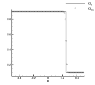
(a) $\alpha_{1}$

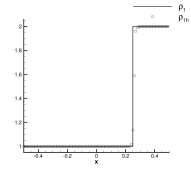
(b) $\rho_{1}$

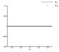
(c) $u_{1}$

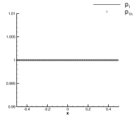
(d) $p_{1}$

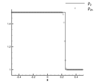
(e) $\rho_{2}$

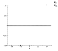
(f) $u_{2}$

(g) $p_{2}$

Figure 2: Comparison of the fourth order accurate numerical solution to the exact solution for test case RP1.

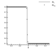
(a) $\alpha_{1}$

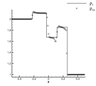
(b) $\rho_{1}$

(c) $u_{1}$

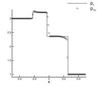
(d) $p_{1}$

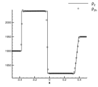
(e) $\rho_{2}$

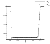
(f) $u_{2}$

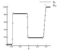
(g) $p_{2}$

Figure 3: Comparison of the fourth order accurate numerical solution to the exact solution for test case RP2.

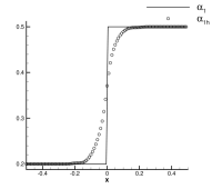
(a) $\alpha_{1}$

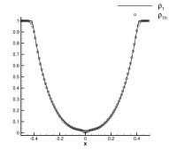
(b) $\rho_{1}$

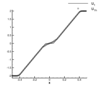
(c) $u_{1}$

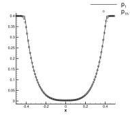
(d) $p_{1}$

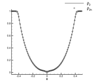
(e) $\rho_{2}$

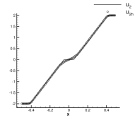
(f) $u_{2}$

(g) $p_{2}$

Figure 4: Comparison of the fourth order accurate numerical solution to the exact solution for test case RP3.

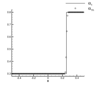
(a) $\alpha_{1}$

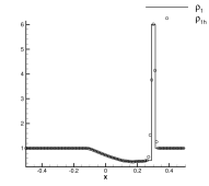
(b) $\rho_{1}$

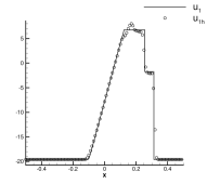
(c) $u_{1}$

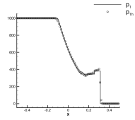
(d) $p_{1}$

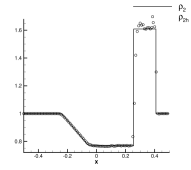
(e) $\rho_{2}$

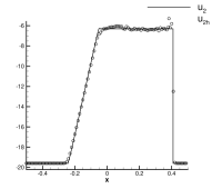
(f) $u_{2}$

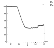
(g) $p_{2}$

Figure 5: Comparison of the fourth order accurate numerical solution to the exact solution for test case RP4.

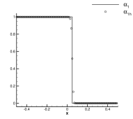
(a) $\alpha_{1}$

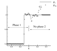
(b) $\rho_{1}$

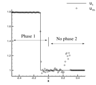
(c) $u_{1}$

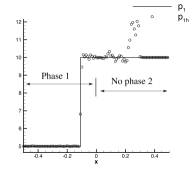
(d) $p_{1}$

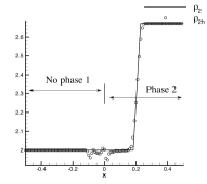
(e) $\rho_{2}$

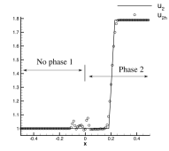
(f) $u_{2}$

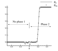
(g) $p_{2}$

Figure 6: Comparison of the fourth order accurate numerical solution to the exact solution for test case RP5.

7 Numerical tests in multiple space dimensions

The Baer-Nunziato model in multiple space dimensions reads

$$\partial_{t}{\textbf{u}}+\nabla\cdot\textbf{f}({\textbf{u}})+\textbf{c}({\textbf{u}})\nabla{\textbf{u}}=0,\quad\textbf{x}\in\mathbb{R}^{d},\,t\geqslant 0,$$ (60)

where

$${\textbf{u}}\mathrel{\mathop{\mathchar 58\relax}}=\begin{pmatrix}\alpha_{i}\\ \alpha_{i}\rho_{i}\\ \alpha_{i}\rho_{i}\textbf{v}_{i}\\ \alpha_{i}\rho_{i}E_{i}\end{pmatrix},\quad\textbf{f}({\textbf{u}})\mathrel{\mathop{\mathchar 58\relax}}=\begin{pmatrix}0\\ \alpha_{i}\rho_{i}\textbf{v}_{i}^{\top}\\ \alpha_{i}(\rho_{i}\textbf{v}_{i}\textbf{v}^{\top}_{i}+\mathrm{p}_{i}\textbf{I})\\ \alpha_{i}(\rho_{i}E_{i}+\mathrm{p}_{i})\textbf{v}_{i}^{\top}\end{pmatrix},\quad\textbf{c}({\textbf{u}})\nabla{\textbf{u}}\mathrel{\mathop{\mathchar 58\relax}}=\begin{pmatrix}\mathrm{\textbf{v}_{I}}^{\top}\\ 0\\ -\mathrm{p_{I}}\textbf{I}\\ -\mathrm{p_{I}}\mathrm{\textbf{v}_{I}}^{\top}\end{pmatrix}\nabla\alpha_{i},\quad i=1,2,$$

with $\textbf{v}_{i}=(u_{i},v_{i},w_{i})^{\top}$ the velocity vector of the $i$th phase, $\mathrm{p}_{i}=\mathrm{p}_{i}(\rho_{i},e_{i})$ given by (eq. 5) and $e_{i}=E_{i}-\tfrac{1}{2}{\bf v}_{i}\cdot{\bf v}_{i}$ the specific internal energy.

The DGSEM scheme (eq. 33) can be extended to (eq. 60). The derivation of the scheme for Cartesian meshes is introduced in A, while the numerical fluxes for the above model are presented in B. Unless stated otherwise, the time step is computed with the CFL condition in C and was seen to maintain positivity of the solution though it does not guaranty positivity of the partial internal energies.

Numerical experiments in two-space dimensions are given in the remainder of this section including tests on high-order accuracy and entropy conservation of the scheme, together with the simulation of a shock-bubble interaction problem.

7.1 Advection of density and void fraction waves

We here reproduce the test on accuracy from section 6.1 and consider the pure advection of oblique void fraction and density waves in a uniform flow in a unit square with periodic boundary conditions. The initial condition reads

$$\alpha_{1,0}({\bf x})=\frac{1}{2}+\frac{1}{4}\sin\big{(}4\pi(x+y)\big{)},\;\rho_{i,0}({\bf x})=1+\frac{1}{2}\sin\big{(}2\pi(x+y)\big{)},\;u_{i,0}({\bf x})=1,\;v_{i,0}({\bf x})=1,\;\mathrm{p}_{i,0}({\bf x})=1,\;i=1,2.$$ (61)

The EOS parameters in (eq. 5) are $\gamma_{i}=1.4$ and $\mathrm{p}_{\infty_{i}}=10$ for $i=1,2$. The obtained results are presented in Table 5. It is again observed that the expected $p+1$ order of convergence is achieved.

$p$	$h$	$\left\lVert e_{h}\right\rVert_{L^{1}(\Omega_{h})}$	$\mathcal{O}_{1}$	$\left\lVert e_{h}\right\rVert_{L^{2}(\Omega_{h})}$	$\mathcal{O}_{2}$	$\left\lVert e_{h}\right\rVert_{L^{\infty}(\Omega_{h})}$	$\mathcal{O}_{\infty}$
1	1/4	3.26E-01	-	4.19E-01	-	6.09E-01	-
	1/8	2.92E-01	0.16	3.36E-01	0.32	5.13E-01	0.25
	1/16	8.40E-02	1.80	9.41E-02	1.84	1.57E-01	1.71
	1/32	1.42E-02	2.56	1.71E-02	2.46	3.39E-02	2.21
	1/64	4.14E-03	1.78	4.91E-03	1.80	1.03E-02	1.72
2	1/4	3.96E-02	-	4.67E-02	-	8.33E-02	-
	1/8	8.75E-03	2.18	1.11E-02	2.07	4.03E-02	1.05
	1/16	1.41E-03	2.63	1.63E-03	2.78	4.57E-03	3.14
	1/32	1.19E-04	3.57	1.58E-04	3.36	4.10E-04	3.48
	1/64	1.23E-05	3.28	1.73E-05	3.19	6.26E-05	2.71
3	1/4	1.64E-02	-	1.88E-02	-	3.11E-02	-
	1/8	2.20E-03	2.90	2.70E-03	2.80	6.96E-03	2.16
	1/16	7.10E-05	4.95	8.90E-05	4.92	2.56E-04	4.60
	1/32	1.35E-06	5.71	1.79E-06	5.64	9.68E-06	4.89
	1/64	6.50E-08	4.38	8.64E-08	4.37	5.21E-07	4.22

Table 5: Test for high-order accuracy with initial condition (eq. 61): different norms of the errors on $\tfrac{1}{2}(\rho_{1}+\rho_{2})$ under grid and polynomial degree refinements and associated orders of convergence at final time $T_{max}=5$.

7.2 Entropy conservation

We also check entropy conservation by using the same procedure as in section 6.2.1 on the unit square with periodic boundary conditions. The initial condition is EC in Table 2 with zero transverse velocity, $v_{i}=0$ for $i=1,2$, and we keep the same EOS parameters. The global entropy budget, similar to (eq. 59), is displayed in Table 6 when refining the time step. Again the conservation of entropy by the space discretization is observed.

time step	$\mathcal{E}_{\Omega}(t)$	$\mathcal{O}$
$\Delta t$	7.49E-04	-
$\Delta t/2$	1.07E-04	2.81
$\Delta t/4$	1.37E-05	2.97
$\Delta t/8$	1.72E-06	2.99
$\Delta t/16$	2.15E-07	3.00
$\Delta t/32$	2.67E-08	3.01
$\Delta t/64$	3.19E-09	3.06

Table 6: Global entropy budget (eq. 59) in two space dimensions and the corresponding order of convergence $\mathcal{O}$.

7.3 Shock-bubble interaction

This numerical test involves the interaction between a shock wave and a material discontinuity. The test was introduced by Haas and Sturtevant [33] to experimentally study the interaction of a shock wave with a single discrete gaseous inhomogeneity. Later it was adopted as a numerical benchmark to validate the robustness and accuracy of various numerical schemes for compressible two-phase flows, see [52, 58, 31, 44, 39, 43, 62, 54] and references therein.

The computational domain $\Omega_{h}=[0,6.5]\times[0,1.78]$ is discretized using a Cartesian mesh with $1300\times 356$ elements. The initial condition involves a bubble of unit diameter containing a mixture of $95\%$ of helium by volume ($\alpha_{1}=0.95$) and $5\%$ of air, to exclude resonance effects (eq. 14), in a domain filled with $5\%$ of air. The center of the bubble is located at ${\bf x}=(3.5,0.89)$. A left moving shock is initially placed at the rightmost edge of the bubble, $x_{0}=4$, and then moves to the left and interacts with the bubble. The initial condition is provided in Table 7.

	$\alpha_{1}$	$\rho_{i}$	$u_{i}$	$v_{i}$	$\mathrm{p}_{i}$
Pre-shock air ($i=2$)	0.05	1.3764	-0.3336	0.0	1.1213
Helium bubble ($i=1$)	0.95	0.1819	0.0	0.0	0.7143
Post-shock air ($i=2$)	0.05	1.0	0.0	0.0	0.7143

Table 7: Physical parameters for the initial condition of the shock-bubble interaction problem.

The EOS parameters for helium and air are $\gamma_{1}=1.648$ and $\mathrm{C_{v}}_{1}=6.06$, and $\gamma_{2}=1.4$ and $\mathrm{C_{v}}_{2}=1.786$, respectively. The physical model does not involve viscous effects so to avoid oscillations of the interface we smoothen the initial condition around the material interface following [44, 38, 7]. The numerical test is performed using periodic boundary conditions at the top and bottom boundaries, and non-reflective conditions on the left and right boundaries.

Figure 7 illustrates the deformation of the He bubble as the shock passes through it. The plotted fields are those of the void fraction for phase 1, the total pressure and numerical Schlieren. It is observed that the material interface and the shock are accurately captured without excessive smearing of the contact. Note however that, for the Baer-Nunziato model, the pressure field shows the presence of a secondary shock inside the bubble (see e.g. the Schlieren at $t=62\mu$s). This secondary shock is due to the presence of air inside the bubble. Furthermore, as the shock leaves the bubble, vortices are generated on the bubble interface as a result of the Kevin-Helmoltz instability.

Figure 8 shows the space-time diagram for three characteristic points on the interface of the bubble. We compare the results obtained with the DGSEM scheme to reference data from [44]. The deformation of the bubble shows complete agreement with the reference data and indicate that the smooth initial condition does not affect the global deformation of the bubble.

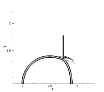
(a) $t=32\mu$s

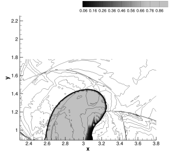
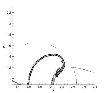
(b) $t=240\mu$s

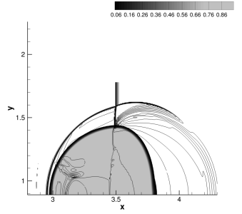
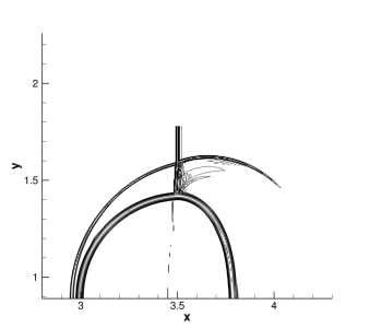
(c) $t=62\mu$s

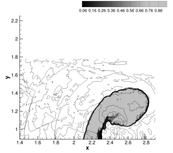
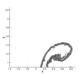
(d) $t=427\mu$s

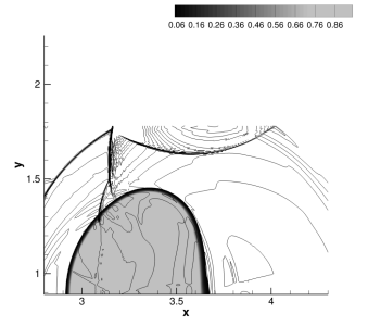
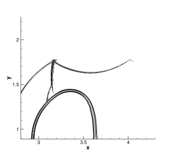
(e) $t=102\mu$s

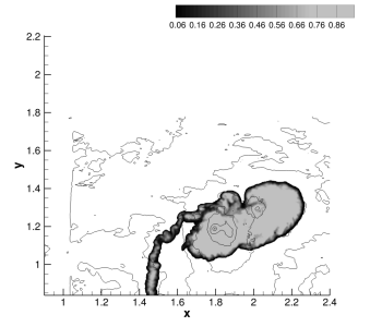
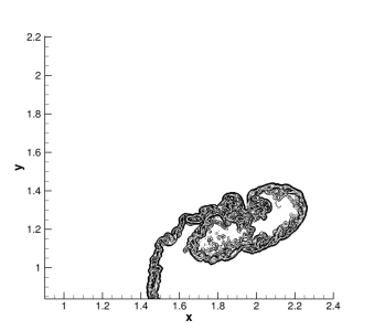
(f) $t=674\mu$s

Figure 7: The snapshots of the deformation of the He bubble due to the left traveling shock at various physical times. For each snapshot, the left plot displays contours of the void fraction $\alpha_{1}$ and of the total pressure $\mathrm{p}=\alpha_{1}\mathrm{p}_{1}+\alpha_{2}\mathrm{p}_{2}$, while the right plot shows the Schlieren $\phi=\exp(|\nabla\rho|/|\nabla\rho|_{\max})$, with $\rho=\alpha_{1}\rho_{1}+\alpha_{2}\rho_{2}$, obtained with a polynomial degree $p=3$.

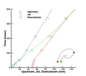
Figure 8: Space-time diagram for three characteristic points on the interface of the He bubble. The solid lines are the reference data from [44], while the symbols are the results obtained with the present DGSEM scheme and a polynomial degree $p=3$.

8 Concluding remarks

In this work, we derive a high-order entropy stable scheme for the Baer-Nunziato model [5, 57] for flows of two separated immiscible fluids in complete disequilibria with respect to the chemical, mechanical, thermal, and thermodynamic processes. Here we focus on the discretization of the convective part of the model and neglect the disequilibria source terms. The exchange of information at the interfaces of the fluids is governed through interface variables of pressure and velocity, for which we choose closure laws [17, 27] that allow the material interface to be associated to a LD field and an entropy inequality in conservative form to be derived from the model. The model is closed with stiffened gas EOS relevant for both gas and liquid phases.

The space discretization is performed by using the semi-discrete entropy stable DGSEM framework proposed in [53], which involves modifying the integration over cell elements by replacing the physical fluxes with two point entropy conservative fluxes in fluctuation form [50, 10], while employing entropy stable fluctuation fluxes at the cell interfaces. This framework is here generalized to include both conservative and nonconservative terms to allow a conservative discretization of the former ones. The entropy conservative fluxes are derived by using the condition in [10], to which we add upwind type dissipation to obtain the entropy stable fluxes. The semi-discrete scheme is high-order accurate for smooth solutions, satisfies an entropy inequality, and is kinetic energy preserving.

We use a method of lines with an explicit time integration and propose conditions on the numerical parameters that guarantee the positivity of the cell-averaged partial densities and a maximum principle on the void fraction for the fully discrete scheme coupled with a first-order forward Euler discretization. High-order integration in time is performed using strong stability-preserving explicit Runge-kutta schemes [59]. The positivity of the solution is then extended to nodal values using a posteriori limiters, inspired from [66, 67, 51].

The numerical tests involve specific test cases that validate the high-order accuracy and entropy conservation of the semi-discrete scheme in one and two space dimensions. Riemann problems are performed in one space dimension involving the development of strong shocks, contacts, near vacuum regions, and vanishing phases. The results obtained with a fourth-order scheme show that the present method captures the physically relevant solution. The intermediate states are well resolved, as well as the shocks and contacts and the computation is shown to be robust in situations close to either vacuum, or resonance. Furthermore, the application to the simulation of a shock-bubble interaction problem in two space dimensions confirm the accurate approximation of the shock and material interfaces.

Appendix A DGSEM in multiple space dimensions

We here extend the DGSEM to multiple space dimensions and restrict ourselves to Cartesian meshes. For the sake of clarity we introduce the scheme in two space dimensions, $d=2$, on uniform grids without loss of generality.

The physical domain $\Omega$ is discretized with a Cartesian grid $\Omega_{h}$ with elements $\kappa_{i,j}=[x_{i-\frac{1}{2}},x_{i+\frac{1}{2}}]\times[y_{j-\frac{1}{2}},y_{j+\frac{1}{2}}]$ with $x_{i+\frac{1}{2}}=ih_{x}$, $y_{j+\frac{1}{2}}=jh_{y}$, where $h_{x}>0$ and $h_{y}>0$ are the space steps.The Cartesian coordinate system is denoted as $(0,{\bf e_{x}},{\bf e_{y}})$. Each element $\kappa_{i,j}$ is defined through the mapping $\textbf{x}_{i,j}\mathrel{\mathop{\mathchar 58\relax}}I^{2}\ni(\xi,\eta)\mapsto{\bf x}=\textbf{x}_{i,j}(\xi,\eta)\in\kappa_{i,j}$ with $I^{2}=[-1,1]^{2}$. The function space $\mathcal{V}^{p}_{h}$ restricted onto an element $\kappa_{i,j}$ is spanned with functions defined as tensor products of one-dimensional Lagrange polynomials associated to the Gauss-Lobatto nodes (see section 3.1):

$$\phi^{kl}_{i,j}\big{(}\textbf{x}_{i,j}(\xi,\eta)\big{)}\mathrel{\mathop{\mathchar 58\relax}}=\ell_{k}(\xi)\ell_{l}(\eta),\quad 0\leqslant k,l\leqslant p,$$

which satisfy the cardinality relation $\ell_{k}(\xi_{\tilde{k}})\ell_{l}(\eta_{\tilde{l}})=\delta_{\tilde{k}k}\delta_{\tilde{l}l}$ for $0\leqslant\tilde{k},k,\tilde{l},l\leqslant p$. The approximate solution is now represented as

$${\textbf{u}}_{h}(\textbf{x},t)\mathrel{\mathop{\mathchar 58\relax}}=\sum^{p}_{k,l=0}\phi^{kl}_{i,j}(\textbf{x})\textbf{U}^{kl}_{i,j}(t)\quad\forall\textbf{x}\in\kappa_{i,j},\;t\geqslant 0.$$

The integrals over the physical elements and faces are approximated with Gauss-Lobatto quadratures:

$$\int_{\kappa_{i,j}}f(\textbf{x})dV\approx\sum^{p}_{k,l=0}\omega_{k}\omega_{l}\frac{h_{x}h_{y}}{4}f(\textbf{x}_{i,j}^{kl}),\quad\int_{e}f(\textbf{x})dS\approx\sum^{p}_{k=0}\omega_{k}\frac{|e|}{2}f(\textbf{x}_{e}^{k}),$$

where $\omega_{k}$ and $\omega_{k}\omega_{l}$ are the Gaussian weights, and $|e|$ is the length of $e$.

The semi-discrete DGSEM for the discretization of (eq. 60) then reads

$$\frac{h_{x}h_{y}}{4}\frac{d{\bf U}_{i,j}^{kl}}{dt} +\omega_{l}\frac{h_{y}}{2}\bigg{(}\sum^{p}_{m=0}\omega_{k}D_{km}\tilde{{\textbf{D}}}(\textbf{U}^{kl}_{i,j},\textbf{U}^{ml}_{i,j},{\bf e_{x}})+\delta_{kp}{\textbf{D}}^{-}(\textbf{U}^{pl}_{i,j},\textbf{U}^{0l}_{i+1,j},{\bf e_{x}})+\delta_{k0}{\textbf{D}}^{+}(\textbf{U}^{pl}_{i-1,j},\textbf{U}^{0l}_{ij},{\bf e_{x}})\bigg{)}$$

$$+\omega_{k}\frac{h_{x}}{2}\bigg{(}\sum^{p}_{m=0}\omega_{l}D_{lm}\tilde{{\textbf{D}}}(\textbf{U}^{kl}_{i,j},\textbf{U}^{km}_{i,j},{\bf e_{y}})+\delta_{lp}{\textbf{D}}^{-}(\textbf{U}^{kp}_{i,j},\textbf{U}^{k0}_{i,j+1},{\bf e_{y}})+\delta_{l0}{\textbf{D}}^{+}(\textbf{U}^{kp}_{i,j-1},\textbf{U}^{k0}_{ij},{\bf e_{y}})\bigg{)}=0,$$

with

$$\tilde{{\textbf{D}}}({\textbf{u}}^{-},{\textbf{u}}^{+},{\bf n})\mathrel{\mathop{\mathchar 58\relax}}={\textbf{D}}^{-}_{ec}({\textbf{u}}^{-},{\textbf{u}}^{+},{\bf n})-{\textbf{D}}^{+}_{ec}({\textbf{u}}^{+},{\textbf{u}}^{-},{\bf n}),$$

and the numerical fluxes are defined in B.

Appendix B Entropy conservative and entropy stable fluxes in multiple space dimensions

In multidimensional space, for solutions belonging to the phase space

$$\Omega_{\scalebox{0.8}{$\scriptscriptstyle\rm BNM$}}=\big{\{}{\textbf{u}}\in\mathbb{R}^{5+2d}\mathrel{\mathop{\mathchar 58\relax}}\,\rho_{i}>0,\,{\bf v}_{i}\in\mathbb{R}^{d},\,e_{i}>0,\,0<\alpha_{i}<1,\;i=1,2\big{\}},$$

the entropy conservative fluxes (eq. 28) are defined as follows:

$${\textbf{D}}^{\mp}_{ec}({\textbf{u}}^{-},{\textbf{u}}^{+},{\bf n})=\pm\textbf{h}({\textbf{u}}^{-},{\textbf{u}}^{+},\textbf{n})\mp\textbf{f}({\textbf{u}}^{\mp})\cdot\textbf{n}+{\textbf{d}}^{\mp}({\textbf{u}}^{-},{\textbf{u}}^{+},\textbf{n}),$$

for the system (eq. 60). They are assumed to be consistent ${\textbf{D}}^{\mp}_{ec}({\textbf{u}},{\textbf{u}},{\bf n})=0$ and are defined as follows:

$${\textbf{h}}({\textbf{u}}^{-},{\textbf{u}}^{+},\textbf{n})\mathrel{\mathop{\mathchar 58\relax}}=\begin{pmatrix}0\\ \displaystyle\hbox to0.0pt{\hskip 0.37865pt\leavevmode\hbox{\set@color$\overline{\hbox{}}$}\hss}{\footnotesize{\leavevmode\hbox{\set@color$\alpha$}}}_{i}\hat{\rho}_{i}\hskip 0.125pt\hbox to0.0pt{\leavevmode\hbox{\set@color$\textbf{v}$}\hss}{\footnotesize{\hskip-0.125pt\leavevmode\hbox{\set@color$\overline{\hbox{}}$}}}_{i}\cdot\textbf{n}\\ \displaystyle\hbox to0.0pt{\hskip 0.37865pt\leavevmode\hbox{\set@color$\overline{\hbox{}}$}\hss}{\footnotesize{\leavevmode\hbox{\set@color$\alpha$}}}_{i}\left(\hat{\rho}_{i}(\hskip 0.125pt\hbox to0.0pt{\leavevmode\hbox{\set@color$\textbf{v}$}\hss}{\footnotesize{\hskip-0.125pt\leavevmode\hbox{\set@color$\overline{\hbox{}}$}}}_{i}\cdot\textbf{n})\hskip 0.125pt\hbox to0.0pt{\leavevmode\hbox{\set@color$\textbf{v}$}\hss}{\footnotesize{\hskip-0.125pt\leavevmode\hbox{\set@color$\overline{\hbox{}}$}}}_{i}+\frac{\hbox to0.0pt{\hskip 3.84883pt\leavevmode\hbox{\set@color$\overline{\hbox{}}$}\hss}{\footnotesize{\leavevmode\hbox{\set@color$\mathrm{p}_{i}\theta_{i}$}}}}{\hskip 0.38751pt\hbox to0.0pt{\leavevmode\hbox{\set@color$\theta$}\hss}{\footnotesize{\hskip-0.38751pt\leavevmode\hbox{\set@color$\overline{\hbox{}}$}}}_{i}}{\textbf{n}}\right)\\ \hbox to0.0pt{\hskip 0.37865pt\leavevmode\hbox{\set@color$\overline{\hbox{}}$}\hss}{\footnotesize{\leavevmode\hbox{\set@color$\alpha$}}}_{i}\left(\hat{\rho}_{i}\left(\displaystyle\frac{\mathrm{C_{v}}_{i}}{\hat{\theta}_{i}}+\frac{\textbf{v}^{-}_{i}\cdot\textbf{v}^{+}_{i}}{2}\right)+\frac{\hbox to0.0pt{\hskip 1.94415pt\leavevmode\hbox{\set@color$\overline{\hbox{}}$}\hss}{\footnotesize{\leavevmode\hbox{\set@color$\mathrm{p}_{i}\theta_{i}$}}}}{\hskip 0.41354pt\hbox to0.0pt{\leavevmode\hbox{\set@color$\theta_{i}$}\hss}{\footnotesize{\hskip-0.41354pt\leavevmode\hbox{\set@color$\overline{\hbox{}}$}}}}+\mathrm{p}_{\infty,i}\right)\hskip 0.125pt\hbox to0.0pt{\leavevmode\hbox{\set@color$\textbf{v}$}\hss}{\footnotesize{\hskip-0.125pt\leavevmode\hbox{\set@color$\overline{\hbox{}}$}}}_{i}\cdot\textbf{n}\end{pmatrix}-\beta_{s}\frac{\llbracket\alpha_{i}\rrbracket}{2}\begin{pmatrix}1\\ \hat{\rho}_{i}\\ \hat{\rho}_{i}\hskip 0.125pt\hbox to0.0pt{\leavevmode\hbox{\set@color$\textbf{v}$}\hss}{\footnotesize{\hskip-0.125pt\leavevmode\hbox{\set@color$\overline{\hbox{}}$}}}_{i}\\ \displaystyle\hat{\rho}_{i}\left(\frac{\mathrm{C_{v}}_{i}}{\hat{\theta}_{i}}+\frac{\textbf{v}^{-}_{i}\cdot\textbf{v}^{+}_{i}}{2}\right)+\mathrm{p}_{\infty,i}\end{pmatrix},$$ (62)

$${\textbf{d}}^{\pm}({\textbf{u}}^{-},{\textbf{u}}^{+},{\bf n})\mathrel{\mathop{\mathchar 58\relax}}=\frac{\llbracket\alpha_{i}\rrbracket}{2}\begin{pmatrix}{\bf v}_{\mathrm{I}}^{\pm}\cdot\textbf{n}\\ 0\\ -\mathrm{p_{I}}^{\pm}{\textbf{n}}\\ -\mathrm{p_{I}}^{\pm}{\bf v}_{\mathrm{I}}^{\pm}\cdot\textbf{n}\end{pmatrix},\quad i\in\{1,2\}.$$

The entropy stable fluxes read

$${\textbf{D}}^{\pm}({\textbf{u}}^{-},{\textbf{u}}^{+},{\textbf{n}})=\textbf{D}^{\pm}_{ec}({\textbf{u}}^{-},{\textbf{u}}^{+},{\textbf{n}})\pm\textbf{D}_{\nu}({\textbf{u}}^{-},{\textbf{u}}^{+},{\textbf{n}}),$$

with

$${\textbf{D}}_{\nu}({\textbf{u}}^{-},{\textbf{u}}^{+},{\textbf{n}})=\frac{\epsilon_{\nu}}{2}\max\big{(}\rho_{\textbf{A}}({\textbf{u}}^{-},{\textbf{n}}),\rho_{\textbf{A}}({\textbf{u}}^{+},{\textbf{n}})\big{)}\begin{pmatrix}0\\ \llbracket\rho_{i}\rrbracket\\ \llbracket\rho_{i}\textbf{v}_{i}\rrbracket\\ \displaystyle\left(\frac{\mathrm{C_{v}}_{i}}{\hat{\theta}_{i}}+\frac{\textbf{v}^{-}_{i}\cdot\textbf{v}^{+}_{i}}{2}\right)\llbracket\rho_{i}\rrbracket+\hbox to0.0pt{\hskip 0.69473pt\leavevmode\hbox{\set@color$\overline{\hbox{}}$}\hss}{\footnotesize{\leavevmode\hbox{\set@color$\rho_{i}$}}}\llbracket E_{i}\rrbracket\end{pmatrix},\quad i\in\{1,2\},$$

where $\epsilon_{\nu}\geqslant 0$ and $\rho_{\textbf{A}}({\textbf{u}},{\textbf{n}})=\max_{i=1,2}(|{\bf v}_{i}\cdot{\bf n}|+c_{i})$.

Appendix C Condition for positivity of the cell-averaged solution in multiple space dimensions

The condition for positivity of the solution is based on the extension of Theorem 5.2. We introduce $\lambda_{x}=\tfrac{\Delta t}{h_{x}}$ and $\lambda_{y}=\tfrac{\Delta t}{h_{y}}$ with $\Delta t>0$ the time step. Let $\rho^{0\leqslant k,l\leqslant p,n}_{i,j}>0,1>\alpha^{0\leqslant k,l\leqslant p,n}_{i,j}>0$, then the cell-averaged partial densities and void fraction are positive, at time $t^{(n+1)}$, under the following CFL condition:

$$(\lambda_{x}+\lambda_{y})\max_{\kappa\in\Omega_{h}}\max_{{\bf u}={\bf u}_{1},{\bf u}_{2}}\max_{0\leqslant m\leqslant p}\Bigg{(} \max_{0\leqslant k\leqslant p}\frac{1}{\omega_{k}}\Bigg{(}\sum_{l=0}^{p}\omega_{l}D_{lk}\mathrm{u_{I}}_{i,j}^{lm}+\delta_{kp}\frac{\beta_{s_{i+1/2}}^{m}-\mathrm{u_{I}}^{pm}_{i,j}}{2}+\delta_{k0}\frac{\beta_{s_{i-1/2}}^{m}+\mathrm{u_{I}}^{0m}_{i,j}}{2}\Bigg{)},$$ (63)

$$\max_{0\leqslant l\leqslant p}\frac{1}{\omega_{l}}\Bigg{(}\sum_{k=0}^{p}\omega_{k}D_{kl}\mathrm{v_{I}}_{i,j}^{mk}+\delta_{lp}\frac{\beta_{s_{j+1/2}}^{m}-\mathrm{v_{I}}^{mp}_{i,j}}{2}+\delta_{l0}\frac{\beta_{s_{j-1/2}}^{m}+\mathrm{v_{I}}^{m0}_{i,j}}{2}\Bigg{)},$$

$$\frac{1}{\omega_{0}}\Big{(}\frac{(\beta_{s_{i-1/2}}^{m}-\hbox to0.0pt{\hskip 0.07605pt\leavevmode\hbox{\set@color$\overline{\hbox{}}$}\hss}{\footnotesize{\leavevmode\hbox{\set@color$u$}}}_{i-1/2}^{m})\hat{\rho}_{i-1/2}^{m}}{2\rho^{0m}_{i,j}}+\frac{\epsilon_{\nu_{i-1/2}}^{m}}{\alpha^{0m}_{i,j}}\Big{)},\frac{1}{\omega_{p}}\Big{(}\frac{(\beta_{s_{i+1/2}}^{m}+\hbox to0.0pt{\hskip 0.07605pt\leavevmode\hbox{\set@color$\overline{\hbox{}}$}\hss}{\footnotesize{\leavevmode\hbox{\set@color$u$}}}_{i+1/2}^{m})\hat{\rho}_{i+1/2}^{m}}{2\rho^{pm}_{i,j}}+\frac{\epsilon_{\nu_{i+1/2}}^{m}}{\alpha^{pm}_{i,j}}\Big{)},$$

$$\frac{1}{\omega_{0}}\Big{(}\frac{(\beta_{s_{j-1/2}}^{m}-\hskip 0.1573pt\hbox to0.0pt{\leavevmode\hbox{\set@color$v$}\hss}{\footnotesize{\hskip-0.1573pt\leavevmode\hbox{\set@color$\overline{\hbox{}}$}}}_{j-1/2}^{m})\hat{\rho}_{j-1/2}^{m}}{2\rho^{m0}_{i,j}}+\frac{\epsilon_{\nu_{j-1/2}}^{m}}{\alpha^{m0}_{i,j}}\Big{)},\frac{1}{\omega_{p}}\Big{(}\frac{(\beta_{s_{j+1/2}}^{m}+\hskip 0.1573pt\hbox to0.0pt{\leavevmode\hbox{\set@color$v$}\hss}{\footnotesize{\hskip-0.1573pt\leavevmode\hbox{\set@color$\overline{\hbox{}}$}}}_{j+1/2}^{m})\hat{\rho}_{j+1/2}^{m}}{2\rho^{mp}_{i,j}}+\frac{\epsilon_{\nu_{j+1/2}}^{m}}{\alpha^{mp}_{i,j}}\Big{)}\Bigg{)}^{(n)}<\frac{1}{2},$$

where

$$\beta_{s_{i+1/2}}^{m} =\max_{i_{p}=1,2}\big{(}|u^{pm,n}_{i_{p},i,j}|,|u^{0m,n}_{i_{p},i+1,j}|\big{)},\quad\beta_{s_{j+1/2}}^{m}=\max_{i_{p}=1,2}\big{(}|v^{mp,n}_{i_{p},i,j}|,|v^{m0,n}_{i_{p},i,j+1}|\big{)},\quad 0\leqslant m\leqslant p,$$

$$\hbox to0.0pt{\hskip 0.07605pt\leavevmode\hbox{\set@color$\overline{\hbox{}}$}\hss}{\footnotesize{\leavevmode\hbox{\set@color$u$}}}_{i+1/2}^{m} =\tfrac{u^{pm,n}_{i,j}+u^{0m,n}_{i+1,j}}{2},\quad\hskip 0.1573pt\hbox to0.0pt{\leavevmode\hbox{\set@color$v$}\hss}{\footnotesize{\hskip-0.1573pt\leavevmode\hbox{\set@color$\overline{\hbox{}}$}}}_{j+1/2}^{m}=\tfrac{v^{mp,n}_{i,j}+v^{m0,n}_{i+1,j}}{2},\quad 0\leqslant m\leqslant p,$$

$$\hat{\rho}_{i+1/2}^{m} =\tfrac{\rho^{0m,n}_{i+1,j}-\rho^{pm,n}_{i,j}}{\ln\rho^{0m,n}_{i+1,j}-\ln\rho^{pm,n}_{i,j}},\quad\hat{\rho}_{j+1/2}^{m}=\tfrac{\rho^{m0,n}_{i,j+1}-\rho^{mp,n}_{i,j}}{\ln\rho^{m0,n}_{i,j+1}-\ln\rho^{mp,n}_{i,j}},\quad 0\leqslant m\leqslant p,$$

where $u$, $v$, and $\rho$ refer either to phase ${\bf u}_{1}$, or to ${\bf u}_{2}$ in (eq. 63).

References

- [1] R. Abgrall, How to prevent pressure oscillations in multicomponent flow calculations: a quasi conservative approach, J. Comput. Phys., 125 (1996), pp. 150–160.
- [2] R. Abgrall and S. Karni, A comment on the computation of non-conservative products, J. Comput. Phys., 229 (2010), pp. 2759–2763.
- [3] A. Ambroso, C. Chalons, and P.-A. Raviart, A Godunov-type method for the seven-equation model of compressible two-phase flow, Comput. Fluids, 54 (2012), pp. 67–91.
- [4] N. Andrianov and G. Warnecke, The Riemann problem for the Baer–Nunziato two-phase flow model, J. Comput. Phys., 195 (2004), pp. 434–464.
- [5] M. Baer and J. Nunziato, A two-phase mixture theory for the deflagration-to-detonation transition (DDT) in reactive granular materials, Int. J. Multiphase Flow, 12 (1986), pp. 861–889.
- [6] C. Berthon, F. Coquel, and P. G. LeFloch, Why many theories of shock waves are necessary: kinetic relations for non-conservative systems, Proc. R. Soc. Edin. A, 142 (2012), pp. 1–37.
- [7] G. Billet, V. Giovangigli, and G. De Gassowski, Impact of volume viscosity on a shock–hydrogen-bubble interaction, Combust. Theory Model., 12 (2008), pp. 221–248.
- [8] M. Bohm, A. Winters, G. Gassner, D. Derigs, F. Hindenlang, and J. Saur, An entropy stable nodal discontinuous Galerkin method for the resistive MHD equations. Part I: Theory and numerical verification, J. Comput. Phys., (2018).
- [9] M. J. Castro, T. M. de Luna, and C. Parés, Well-balanced schemes and path-conservative numerical methods, in Handbook of Numer. Anal., vol. 18, Elsevier, 2017, pp. 131–175.
- [10] M. J. Castro, U. S. Fjordholm, S. Mishra, and C. Parés, Entropy conservative and entropy stable schemes for nonconservative hyperbolic systems, SIAM J. Numer. Anal., 51 (2013), pp. 1371–1391.
- [11] M. J. Castro, J. Gallardo, and C. Parés, High order finite volume schemes based on reconstruction of states for solving hyperbolic systems with nonconservative products. applications to shallow-water systems, Math. Comput., 75 (2006), pp. 1103–1134.
- [12] M. J. Castro, P. G. LeFloch, M. L. Muñoz-Ruiz, and C. Parés, Why many theories of shock waves are necessary: Convergence error in formally path-consistent schemes, J. Comput. Phys., 227 (2008), pp. 8107–8129.
- [13] M. J. Castro, C. Parés, G. Puppo, and G. Russo, Central schemes for nonconservative hyperbolic systems, SIAM J. Sci. Comput., 34 (2012), pp. B523–B558.
- [14] C. Chalons and F. Coquel, A new comment on the computation of non-conservative products using Roe-type path conservative schemes, J. Comput. Phys., 335 (2017), pp. 592 – 604.
- [15] P. Chandrashekar, Kinetic energy preserving and entropy stable finite volume schemes for compressible Euler and Navier-Stokes equations, Commun. Comput. Phys., 14 (2013), pp. 1252–1286.
- [16] T. Chen and C.-W. Shu, Entropy stable high order discontinuous galerkin methods with suitable quadrature rules for hyperbolic conservation laws, J. Comput. Phys., 345 (2017), pp. 427–461.
- [17] F. Coquel, T. Gallouët, J.-M. Hérard, and N. Seguin, Closure laws for a two-fluid two-pressure model, C. R. Acad. Sci. Paris, 334 (2002), pp. 927–932.
- [18] F. Coquel, J.-M. Hérard, and K. Saleh, A positive and entropy-satisfying finite volume scheme for the Baer–Nunziato model, J. Comput. Phys., 330 (2017), pp. 401–435.
- [19] G. Dal Maso, P. Le Floch, and F. Murat, Definition and weak stability of nonconservative products, J. Math. Pures Appl., 74 (1995), pp. 483–548.
- [20] D. A. Drew and S. L. Passman, Theory of multicomponent fluids, vol. 135, Springer Science & Business Media, 2006.
- [21] M. Dumbser and W. Boscheri, High-order unstructured Lagrangian one-step WENO finite volume schemes for non-conservative hyperbolic systems: applications to compressible multi-phase flows, Comput. Fluids, 86 (2013), pp. 405–432.
- [22] M. Dumbser, M. Castro, C. Parés, and E. F. Toro, ADER schemes on unstructured meshes for nonconservative hyperbolic systems: Applications to geophysical flows, Comput. Fluids, 38 (2009), pp. 1731–1748.
- [23] M. Dumbser and E. F. Toro, A simple extension of the Osher Riemann solver to non-conservative hyperbolic systems, SIAM J. Sci. Comput., 48 (2011), pp. 70–88.
- [24] T. C. Fisher and M. H. Carpenter, High-order entropy stable finite difference schemes for nonlinear conservation laws: Finite domains, J. Comput. Phys., 252 (2013), pp. 518–557.
- [25] E. Franquet and V. Perrier, Runge–Kutta discontinuous Galerkin method for the approximation of Baer and Nunziato type multiphase models, J. Comput. Phys., 231 (2012), pp. 4096–4141.
- [26] F. Fraysse, C. Redondo, G. Rubio, and E. Valero, Upwind methods for the Baer–Nunziato equations and higher-order reconstruction using artificial viscosity, J. Comput. Phys., 326 (2016), pp. 805–827.
- [27] T. Gallouët, J.-M. Hérard, and N. Seguin, Numerical modeling of two-phase flows using the two-fluid two-pressure approach, Math. Models Methods Appl. Sci., 14 (2004), pp. 663–700.
- [28] G. J. Gassner, A skew-symmetric discontinuous Galerkin spectral element discretization and its relation to SBP-SAT finite difference methods, SIAM J. Sci. Comput., 35 (2013), pp. A1233–A1253.
- [29] G. J. Gassner, A kinetic energy preserving nodal discontinuous Galerkin spectral element method, Int. J. Numer. Methods Fluids, 76 (2014), pp. 28–50.
- [30] G. J. Gassner, A. R. Winters, and D. A. Kopriva, Split form nodal discontinuous Galerkin schemes with summation-by-parts property for the compressible Euler equations, J. Comput. Phys., 327 (2016), pp. 39–66.
- [31] J. Giordano and Y. Burtschell, Richtmyer-Meshkov instability induced by shock-bubble interaction: Numerical and analytical studies with experimental validation, Phys. Fluids, 18 (2006), p. 036102.
- [32] S. Gottlieb, C.-W. Shu, and E. Tadmor, Strong stability-preserving high-order time discretization methods, SIAM review, 43 (2001), pp. 89–112.
- [33] J.-F. Haas and B. Sturtevant, Interaction of weak shock waves with cylindrical and spherical gas inhomogeneities, J. Fluid Mech., 181 (1987), pp. 41–76.
- [34] A. Harten, P. D. Lax, and B. V. Leer, On upstream differencing and Godunov-type schemes for hyperbolic conservation laws, SIAM review, 25 (1983), pp. 35–61.
- [35] A. Hiltebrand and S. Mishra, Entropy stable shock capturing space–time discontinuous Galerkin schemes for systems of conservation laws, Numer. Math., 126 (2014), pp. 103–151.
- [36] A. Hiltebrand, S. Mishra, and C. Parés, Entropy-stable space–time DG schemes for non-conservative hyperbolic systems, ESAIM: M2AN, 52 (2018), pp. 995–1022.
- [37] S. Hou and X.-D. Liu, Solutions of multi-dimensional hyperbolic systems of conservation laws by square entropy condition satisfying discontinuous Galerkin method, J. Sci. Comput., 31 (2007), pp. 127–151.
- [38] R. W. Houim and K. K. Kuo, A low-dissipation and time-accurate method for compressible multi-component flow with variable specific heat ratios, J. Comput. Phys., 230 (2011), pp. 8527–8553.
- [39] X. Y. Hu, B. Khoo, N. A. Adams, and F. Huang, A conservative interface method for compressible flows, J. Comput. Phys., 219 (2006), pp. 553–578.
- [40] F. Ismail and P. L. Roe, Affordable, entropy-consistent Euler flux functions ii: Entropy production at shocks, J. Comput. Phys., 228 (2009), pp. 5410–5436.
- [41] A. Jameson, Formulation of kinetic energy preserving conservative schemes for gas dynamics and direct numerical simulation of one-dimensional viscous compressible flow in a shock tube using entropy and kinetic energy preserving schemes, J. Sci. Comput., 34 (2008), pp. 188–208.
- [42] G. S. Jiang and C.-W. Shu, On a cell entropy inequality for discontinuous Galerkin methods, Math. Comput., 62 (1994), pp. 531–538.
- [43] E. Johnsen and T. Colonius, Implementation of WENO schemes in compressible multicomponent flow problems, J. Comput. Phys., 219 (2006), pp. 715–732.
- [44] S. Kawai and H. Terashima, A high-resolution scheme for compressible multicomponent flows with shock waves, Int. J. Numer. Methods. Fluids, 66 (2011), pp. 1207–1225.
- [45] D. A. Kopriva and G. Gassner, On the quadrature and weak form choices in collocation type discontinuous Galerkin spectral element methods, J. Sci. Comput., 44 (2010), pp. 136–155.
- [46] Y. Kuya, K. Totani, and S. Kawai, Kinetic energy and entropy preserving schemes for compressible flows by split convective forms, J. Comput. Phys., 375 (2018), pp. 823–853.
- [47] P. Lax and B. Wendroff, Systems of conservation laws, Comm. Pure Appl. Math., 13 (1960), pp. 217–237.
- [48] P. G. LeFloch and S. Mishra, Numerical methods with controlled dissipation for small-scale dependent shocks, Acta Numerica, 23 (2014), pp. 743–816.
- [49] Y. Liu, C.-W. Shu, and M. Zhang, Entropy stable high order discontinuous galerkin methods for ideal compressible MHD on structured meshes, J. Comput. Phys., 354 (2018), pp. 163–178.
- [50] C. Parés, Numerical methods for nonconservative hyperbolic systems: a theoretical framework., SIAM J. Numer. Anal., 44 (2006), pp. 300–321.
- [51] B. Perthame and C.-W. Shu, On positivity preserving finite volume schemes for euler equations, Numer. Math., 73 (1996), pp. 119–130.
- [52] J. J. Quirk and S. Karni, On the dynamics of a shock–bubble interaction, J. Fluid Mech., 318 (1996), pp. 129–163.
- [53] F. Renac, Entropy stable dgsem for nonlinear hyperbolic systems in nonconservative form with application to two-phase flows, J. Comput. Phys., 382 (2019), pp. 1–26.
- [54] F. Renac, Entropy stable, robust and high-order DGSEM for the compressible multicomponent Euler equations, submitted, (2020).
- [55] F. Renac, M. de la Llave Plata, E. Martin, J. B. Chapelier, and V. Couaillier, Aghora: A High-Order DG Solver for Turbulent Flow Simulations, Springer International Publishing, Cham, 2015, pp. 315–335.
- [56] S. Rhebergen, O. Bokhove, and J. J. van der Vegt, Discontinuous Galerkin finite element methods for hyperbolic nonconservative partial differential equations, J. Comput. Phys., 227 (2008), pp. 1887–1922.
- [57] R. Saurel and R. Abgrall, A multiphase Godunov method for compressible multifluid and multiphase flows, J. Comput. Phys., 150 (1999), pp. 425–467.
- [58] R. Saurel, S. Gavrilyuk, and F. Renaud, A multiphase model with internal degrees of freedom: application to shock–bubble interaction, J. Fluid Mech., 495 (2003), pp. 283–321.
- [59] C.-W. Shu and S. Osher, Efficient implementation of essentially non-oscillatory shock-capturing schemes, J. Comput. Phys., 77 (1988), pp. 439–471.
- [60] Z. Sun, J. A. Carrillo, and C.-W. Shu, An entropy stable high-order discontinuous Galerkin method for cross-diffusion gradient flow systems, arXiv preprint arXiv:1810.03221, (2018).
- [61] E. Tadmor, The numerical viscosity of entropy stable schemes for systems of conservation laws. I, Math. Comput., 49 (1987), pp. 91–103.
- [62] H. Terashima and G. Tryggvason, A front-tracking/ghost-fluid method for fluid interfaces in compressible flows, J. Comput. Phys., 228 (2009), pp. 4012–4037.
- [63] S. Tokareva and E. F. Toro, HLLC-type Riemann solver for the Baer–Nunziato equations of compressible two-phase flow, J. Comput. Phys., 229 (2010), pp. 3573–3604.
- [64] N. Wintermeyer, A. R. Winters, G. J. Gassner, and D. A. Kopriva, An entropy stable nodal discontinuous galerkin method for the two dimensional shallow water equations on unstructured curvilinear meshes with discontinuous bathymetry, J. Comput. Phys., 340 (2017), pp. 200–242.
- [65] A. R. Winters and G. J. Gassner, Affordable, entropy conserving and entropy stable flux functions for the ideal MHD equations, J. Comput. Phys., 304 (2016), pp. 72–108.
- [66] X. Zhang and C. Shu, On positivity-preserving high order discontinuous Galerkin schemes for compressible Euler equations on rectangular meshes, J. Comput. Phys., 229 (2010), pp. 8918–8934.
- [67] X. Zhang and C.-W. Shu, On maximum-principle-satisfying high order schemes for scalar conservation laws, J. Comput. Phys., 229 (2010), pp. 3091–3120.