The three-dimensional instabilities and destruction of the Hill’s vortex

Abstract

The Hill vortex is a three-dimensional vortex structure solution of the Euler equations. For small amplitude axisymmetric disturbances on the external surface from the linear stability analysis by Moffat & Moore (1978) emerged the formation of a tail. Successive studies confirmed this fact, and in addition observed a different shape of the tail with azimuthal small amplitude disturbances. In this paper the Navier-Stokes equations are solved at high values of the Reynolds number imposing large amplitude axisymmetric and three-dimensional disturbances on the surface of the vortex. The conclusion is that the azimuthal disturbances produce a hierarchy of structures inside the vortex maintaining the shape of the vortex. On the other hand the axisymmetric disturbances are convected in the rear side, are dumped and form an axisymmetric wave longer higher the magnitude of the surface disturbance. Simulations in a moving frame allow to extend the evolution in time leading to the conclusion that the Hill vortex is unstable and produces a wide range of energy containing scales characteristic of three-dimensional flows.

1 Introduction

The most studied mechanism by which a vortex may become unstable, concern with an inviscid instability which emerges when a vortex is strained, either by other vortices, or as in the case of a vortex ring, by other portions of the curved vortex itself. The long wave instability of a pair of counterotating longitudinal vortices, theoretically explained by Crow (1970) and reproduced in the laboratory by Leweke & Williamson (1998) is an example of the former mechanism. In presence of disturbances of greater amplitude the strain produced by one of the vortices in the dipole affects the other and vice versa producing a sinusoidal modulation along the length of the dipole that results in large-amplitude small-scale vortical structures that strongly deform the primary vortices. This is the short-wave cooperative-instability that should be generated to rapidly destroy the trailing vortices behind aircraft (Orlandi et al. (2001)). A theoretical study of the formation of azimuthal instabilities on vortex rings was given by Widnall et al. (1974). Their predictions were verified by simulations of the Navier-Stokes equations by Shariff et al. (1994). At high Reynolds number the vortex ring when a range of small disturbances at wave numbers different from the most unstable are added may reach a turbulent state. In order to reach the turbulent state the simulation should follow the ring for a long distance requiring a large computational cost. To accelerate this process it may let the ring to impinge a solid wall. Orlandi & Verzicco (1993) described this interaction that is characterised by the creation of vorticity patches on a wide range of scales leading to a rapid destruction of the initial vortex ring. Ren & Lu (2015) at higher Reynolds number reached a fully turbulent condition that was corroborated by energy spectra decaying following a characteristic $k^{-5/3}$ power law. Moreover, they found that the major contribution to the turbulent kinetic energy comes from the azimuthal component that is mainly distributed in the core region of vortex rings.

The vortex introduced by Hill (1894) differently than vortex rings is a solution of the 3D Euler equations preserving its shape while is moving with a constant velocity. The cylindrical coordinate system $(\theta,r,z)$ is the most appropriate coordinate system for its study. The azimuthal vorticity $\omega_{\theta}$ varies with $\sigma=\sqrt{r^{2}+(z-z_{0})^{2}}$ within a spherical region of radius $a$ centered at $z=z_{0}$. Outside $\omega_{\theta}=0$ the consequent sharp interface can not be reproduced numerically in the solution of the Euler equations. Several approaches to study the instability of inviscid vortices are mentioned in the introduction of Protas & Elcrat (2016), therefore are not reported in this paper. Here we are interested to solve the full set of Navier-Stokes equations at the highest possible Reynolds number. This number is chosen in such a way to reproduce and maintain for a sufficient time the interface at the surface of the vortex as sharp as possible. The previous studies were focused on the linearised response of the vortex to perturbation applied on its external surface. For instance Moffat & Moore (1978) derived a set of ordinary differential equations, through a linear perturbation theory, that allows to analyse the time evolution of axisymmetric disturbances of the surface. They found that, depending on the shape of the disturbance, a sharp spike directed into or out the vortex is localised at the rear stagnation point. The same conclusions were reached by the computations of Pozrikidis (1986) of the non-linear regime. Fukuyu et al. (1994) considered non-axisymmetric disturbances leading to results consistent with those by Moffat & Moore (1978). They concluded that spikes form, and that their number is equal to the azimuthal wave number of the perturbation. Rozi (1999) by imposing small scale disturbances reached the same conclusion on the deformation at the rear stagnation point. They also found that the oscillatory motion at the front observed in presence of polar disturbances disappears by adding azimuthal disturbances. They conclude that the Hill vortex subjected to small disturbances is unstable, and that the exponential growth of the spike by varying the azimuthal wave number remains to be clarified, as well as to study the instability at the interior of the vortex.

The present study is devoted to understanding better the obscure points before mentioned. Since any numerical method can not resolve a discontinuous vorticity field a smoothing should be used to let the initial $\omega_{\theta}$ to go to zero outside the surface. Stanaway et al. (1988) to reproduce the collision of two Hill’s vortices through pseudo-spectral methods applied the smoothing to overcome the abrupt jump between the vortical and the irrotational regions. The smoothing function, was introduced by Melander et al. (1987) in two-dimensional simulations to connect the inner to the outer values of the vorticity within a layer of thickness $\delta$. The amplitude of this layer can be varied in amplitude with radial and azimuthal wave numbers, to mimic surface disturbances.

On solving the Navier-Stokes equations, a first consideration should be done on which is the appropriate value of the Reynolds number in order to be as close as possible to an inviscid simulation. The first check of the accuracy and of the quality of the numerical method implies that by inserting large axisymmetric disturbances on the surface the vortex must remain axisymmetric in a fully three-dimensional simulation. This occurrence can be corroborated by proving that the other two vorticity components remain equal to zero. On the other hand, when a combination of axisymmetric and azimuthal disturbances are assigned the direct numerical simulation allow to understand in which region of the vortex the secondary vorticity components grow and become large enough to destroy the spherical shape of the Hill vortex. In addition it can be understood whether are generated flow structures characteristic of fully turbulent flows as those in the viscous collision of two orthogonal Lamb dipoles (Orlandi et al. (2012)). An efficient numerical method in presence of a single wave number excited should maintain the initial symmetries, and the comparison with the random wave number disturbances allows to establish whether the destruction of the Hill vortex is enhanced or not. The response of the Hill vortex to large amplitude disturbances allow to investigate whether similar conclusion of those obtained with the assumption of a linear instability analysis are reached. The further advantage of the DNS is the possibility to look at the evolution of the flow inside the vortex, to understand the mechanism transferring the disturbances in space and to look at the preferential growth of secondary vorticity in certain region. That is to study the entire process leading to the complete destruction of the main vorticity distribution characteristic of the Hill vortex.

2 Numerical scheme

In three-dimension the Navier-Stokes equations in primitive variables reduces the number of operations to advance the solution. In cylindrical coordinates, the definition of the variables $q_{\theta}=rv_{\theta},\ \ \ q_{r}=rv_{r},\ \ \ q_{z}=v_{z}$, as done by Orlandi & Fatica (1997) leads to the equation in Chapt.10 of Orlandi (2000). The discretization of the equation does not differ from that described in Verzicco & Orlandi (1996) where the variable $v_{\theta}$. was used. The quantities $q_{i}$ do not have the same physical dimensions, and this could be a matter of confusion. We wish to point out that these variables were introduced for numerical reasons. The introduction of $q_{r}$ simplifies the treatment of the singularity at $r=0$, and $q_{\theta}$ gives a better accuracy near the axis. In the present simulations an external free-slip boundary has been assumed at a distance equal to $\pi/a$, as in Orlandi & Fatica (1997) periodicity holds in $z$, with $-\pi<z<\pi$. Even if finite differences allow to cluster the grid points in regions of high gradients here an uniform grid in $r$ has been used.

The numerical scheme is described in Chapt.10 of Orlandi (2000) here the main features of the method are summarised. Viscous and advective terms are discretized by centred second order schemes. In the three-dimensional case, in the limit of $\nu\rightarrow 0$, energy is conserved by the discretized equations. The system of equations was solved by a fractional step method. In a first step a non-solenoidal velocity field $\hat{q}_{i}$ is computed, and, if the pressure gradients at the previous time step are retained, the boundary conditions for $\hat{q}_{i}$ are simplified. A scalar quantity $\Phi$ is introduced to project the non-solenoidal field onto a solenoidal one. The large band matrix associated to the elliptic equation for $\Phi$ is reduced to a tridiagonal matrix by periodic $FFTs$ in the azimuthal and in the axial directions. This procedure is very efficient for obtaining the solenoidal velocity. The updated pressure is computed from the scalar $\Phi$. A third order Runge-Kutta scheme, introduced by Wray (1987), was used to advance in time through three sub-steps. The viscous terms are treated implicitly by the Crank-Nicolson scheme. The equation are made dimensionless by taking the radius of the vortex $a$ and a reference velocity linked to the vorticity distribution given in the next section.

3 Initial conditions

The Hill vortex at $t=0$ is centered on the axis at $z=z_{0}=-0.5\pi$. The distribution of the unperturbed $\omega_{\theta}$, if $\sigma=\sqrt{r^{2}+(z-z_{0})^{2}}$, is

$$\omega_{\theta}=\lambda\sigma\left\{\begin{array}[]{ll}1{\hskip 42.67912pt}&\sigma\leq a_{i}\\ 1-f(\xi){\hskip 11.38092pt}&a_{i}\leq\sigma<a_{e}\\ 0{\hskip 42.67912pt}&a_{e}<\sigma\end{array}\right.$$ (4)

where $f(\xi)$ is the smoothing function ($f(\xi)=0$ for $\sigma=a_{i}$ and $f(\xi)=1$ for $\sigma=a_{e}$, with $a_{i}=a-\delta_{0}/2$ and $a_{e}=a+\delta_{0}/2$) defined by Melander et al. (1987), that connects the inner to the outer values of the vorticity. $\lambda$ is a constant related to the uniform stream velocity at infinity ($\lambda=-15U/2a^{2}$) of a irrotational flow past a sphere of radius $a$. The vortex therefore, if $\lambda=1$ moves with a constant velocity $U=2a^{2}/15$. The circulation of the unperturbed vortex is equal to $\Gamma_{0}=2/3$, therefore the reference circulation can be assumed equal to $\Gamma_{*}=3\Gamma_{0}/2$ and the Reynolds number is $Re=\Gamma_{*}/\nu$ with $\nu$ the kinematic viscosity.

The disturbance on the surface of the vortex is assigned by varying the thickness $\delta_{0}=a_{e}-a_{1}$ of $f(\xi)$ through azimuthal $n_{a}$ and polar $n_{p}$ wave numbers. By taking a spherical reference system ($\sigma,\phi,\theta$) located at center of the vortex the smoothing function $f(\xi)$ is applied in the narrow layer $\delta=\delta_{0}\cos(n_{p}\theta)\sin(n_{a}\phi)$.

3.1 Reynolds number effect

\psfrag{ylab}{$z_{c}-z_{5}$}\psfrag{xlab}{ $t-5$}\includegraphics[width=227.62204pt]{fig1b.eps}

\psfrag{ylab}{$z_{c}-z_{5}$}\psfrag{xlab}{ $t-5$}\psfrag{ylab}{$\omega_{\theta}$}\psfrag{xlab}{ $r$}\includegraphics[width=227.62204pt]{fig1a.eps}

a)                                                                 b)

Figure 1: Hill vortex with $\delta_{0}=0.01$ and $n_{p}=n_{a}=0$, a) time evolution of the center of the vortex, b) profile of $\omega_{\theta}$ versus $r$ at $z=z_{c}$ at $t=20$, the solid symbols indicate the values obtained at the $Re$ indicated in the legend.

As above mentioned the three-dimensional viscous simulations should be performed at a $Re$ number giving solutions not too different from the theoretical ones in the inviscid case, and that without any disturbance there is no any growth of the other two vorticity components set equal to zero at $t=0$. A coarse grid $128\times 128\times 256$ respectively in the $\theta$ $r$ and $z$ directions was used at $Re=3000$, on the other hand, at higher $Re$ numbers the grid was $192\times 384\times 768$ for the small $\delta_{0}$ and for others it was increased to $256\times 512\times 1024$. With this mesh approximately $330$ in $z$ and $160$ grid points in $r$ are used to describe the vortex at $t=0$. The small amount of viscosity helps to have an interface accurately described by the mentioned grids. A first validation of the numerical method and of the influence of the viscosity can be performed by comparing the distance travelled by the vortex with the theoretical one determined by $U=2/15$. The distance $z_{c}-z_{0}$ is evaluated by the discrete location of the maximum vorticity. Figure 1a shows that at any value of $Re$ there is a good agreement between the present one and that ($z_{c}-z_{5}=2/15(t-5)$) in the inviscid case. The inset of this figure explains why the first $5$ time units are neglected. In fact, for any $Re$ number, the oscillations on the $z_{c}$ are due to the inaccurate evaluation of the center of the vortex, and also to the small amount of vorticity shed during the motion. The small differences in figure 1a therefore are due to the reduction of circulation due to the effect of the viscosity and to the small amount of vorticity lost by the inaccurate representation of the sharp interface at the boundary of the vortex. This is emphasised in figure 1b by the very large oscillations at $Re=600000$, that disappear at $Re=3000$ and become reasonable at $Re=30000$ and $Re=60000$. In addition, this figure shows that the viscosity affects the vorticity profile not only at the edge but also in the central region. At $t=20$ the large smoothing at the edge, and the high deviation from the linear profile for $0<r<5$ indicates that the results at $Re=3000$ should be quite far from those in the inviscid case. The deviation from the $\omega_{\theta}=r$ profile near the axis does not change much going from $Re=30000$ to $Re=600000$. On the other hand, the oscillations near the edge of the vortex, those we are mainly interested, at $Re=600000$ are too large. In both regions a good compromise is obtained at $Re=60000$ that has been used in all the perturbed simulations described in the next sections.

3.2 Polar perturbations

Moffat & Moore (1978) assigned a linear disturbance combination of Legendre polynomials demonstrating that for prolate disturbances the vortex detrained an amount of vorticity proportional to the disturbance, that had a form of a spike growing in time at the rear stagnation point. The same results were obtained by Pozrikidis (1986) by large amplitude disturbances. Initially the present simulations are devoted to considering polar disturbances on the surface and to compare the evolution with that of the unperturbed vortices. The vortex perturbed with a $n_{p}=16$ wave number travels for $30$ dimensionless time units corresponding to $t^{*}=Ut/a=2.66$. In figure 2 of Pozrikidis (1986) it can be estimated that the size of the spike is approximately equal to the radius of the vortex. In figure 2 the contours of $\omega_{\theta}=0.05$ at $t=0,6,12$ and $t=20$ show the growth of the spike around the rear stagnation point. Even without polar disturbances the spike forms and grows in the rear back of the vortex (figure 2a). This fact can be understood by considering that the smoothing function $f(\xi)$ acts as a disturbance of the inviscid solution. The polar disturbance with $n_{p}=16$ barely visible on the surface at $t=0$ (black line), while the vortex travels, is advected backward along the external boundary, and in figure 2b, at $t=6$, the polar undulations are accumulated in the rear. On the other hand, at the front the surface is smooth and equal to that in figure 2a at the same time.

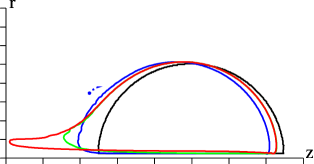
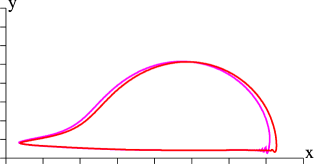
a)                                               b) \psfrag{ylab}{$z_{F}-z_{R}$}\psfrag{xlab}{ $t^{*}$}\includegraphics[width=156.49014pt]{fig2c.eps}                              c)                                               d)

Figure 2: Contour of $\omega_{\theta}=0.05$ at $t=0$ black, $t=6$ blue $t=12$ green and $t=20$ red for a) unperturbed $\delta_{0}=0.01$ ,b) perturbed $\delta_{0}=0.01$ and $n_{p}=16$, c) $\omega_{\theta}=0.05$ at $t=30$ for unperturbed (red) and perturbed (magenta), $r$ varies from $0$ to $1.5$ and $-2<z-z_{c}<1.0$; d) time evolution of the distance between the front and the rear back black $n_{p}=0$, blue $n_{p}=16$ and red dots from figure 2 Pozrikidis (1986).

The amplitude of the undulation grows in time during its translation, in fact it was small at $t=0$, and quite large at $t=6$ (blue line). Later on the perturbation as well as the size of the spike continue to grow, and the undulations are accumulated on the surface of the spike (green line). At this high Reynolds number these oscillations are not damped by the viscosity and at $t=20$ produce a spike with shape different from that without disturbances (red lines). However at $t=30$ has been noticed that these disappear in the wake and the vortices without and with polar disturbances have a similar form (figure 2c). The difference in figure 2c between the perturbed and unperturbed simulations are mainly visible at the front, in fact the vortex with polar disturbances presents oscillations greater than those in the unperturbed case. This oscillatory motion at the front was also found by Rozi (1999). In the inviscid simulations the form of the wake, after the vortex has moved for a long distance, at the rear, in the point where it is attached to the vortex, shrinks considerably. Figure 2a and figure 2b show that in the present viscous simulation this sort of pinch-off does not occur. However, the extension of the spike measured as the distance from the front of the vortex up to the end of the spike in Pozrikidis (1986) agrees well with the present unperturbed and perturbed $n_{p}=16$ results (figure 2d).

3.3 Surface with azimuthal and polar perturbations

Rozi (1999) perturbed the surface of the vortex with small amplitude azimuthal disturbances, they presented the evolution of the surface at different time in their figure 6 with $n_{a}=3$ and in figure 7 with $n_{a}=4$. The inviscid results strengthened the modulation of the spike by the azimuthal disturbance on the surface. In the present simulations disturbances with $n_{a}=1,2,4$ and $n_{a}=8$ have been added to the previous discussed axisymmetric disturbance with $n_{p}=16$. The combination of polar and azimuthal disturbance implies that we are dealing with a three-dimensional flow, therefore the simulations allow to investigate whether and how the disturbances propagate from the surface inside the vortex and in the attached spike. If the amplitude of the disturbances do not grow it may be asserted that the initial structure of the vortex is preserved even if modifications of the surface, for instance the above discussed spike, occur. On the other hand, if the disturbances grow in magnitude there is a probability that the vortex breaks in a wide range of scales. This is the typical mechanism characterising the transition from laminar to turbulent flows.

By imposing disturbances with a single wave number the initial symmetry in the azimuthal direction should be preserved. This a further satisfactory test required to validate any numerical method applied to the Navier-Stokes equation written in polar coordinates. For the simulations discussed in this section with azimuthal disturbances of amplitude $\delta_{0}=0.01$ the resolution ($192\times 384\times 768$), i in the previous section, is maintained. The DNS allow to look in detail at the effects produced by the variation of $n_{a}$ on the distribution of the vorticity components in planes normal to the streamwise motion. Before, however it is worth to looking at the global effects of the three-dimensional disturbances on the azimuthally averaged vorticity components defined as $<\omega_{j}>(r,z)=\frac{\Sigma_{i}}{N_{1}}\omega_{j}$, having also verified that $<\omega_{r}>=<\omega_{z}>=0$.

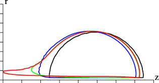
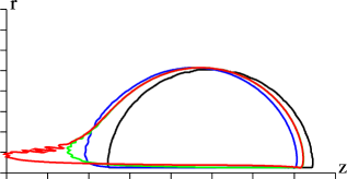
a)                                               b)                                    c)                                               d)

Figure 3: Contour of $<\omega_{\theta}>=0.05$ at $t=0$ black, $t=6$ blue $t=12$ green and $t=20$ red for $\delta_{0}=0.01$ limits as in figure 2: a) $n_{a}=1$, b) $n_{a}=2$, c) $n_{a}=4$ and d) $n_{a}=8$.

Figure 3 similarly to figure 2 shows the contours of $<\omega_{\theta}>$ at the four $n_{a}$ considered. The comparison between the contours in figure 3 an those in figure 2b , at a first glance, shows that by adding azimuthal disturbances the amplitude of the polar disturbances, while these are transported towards the rear stagnation point, is reduced. As a consequence the wake at $t=12$ (green line) does not have the large amplitude disturbances depicted in figure 2b, and the spike has a form similar to that of the unperturbed vortex in figure 2a. At the end of the simulation for $t=20$, at any value of $n_{a}$, the red lines in in figure 3 show that the amplitude of the disturbances in the spike has been largely reduced and becomes smaller lower $n_{a}$ is.

The linear and non-linear instability analysis demonstrated that spikes of different shape form at the rear stagnation point, but can not describe the distribution of the vorticity field at their interior and also, as before mentioned, inside the vortex. The DNS does not have these limitations and allows to understand better, during the evolution, the transfer of the effects of the disturbances from the surface to any region of the Hill vortex. Since a lot of emphasis in the previous studies was devoted to the spike formation, in figure 4 a zoom of the rear region of the vortex is presented at $t=20$. This is the time at which in figure 3 the red lines $<\omega_{\theta}>=0.05$ are plotted. The complex shape of the true spike can not be described by contours of $<\omega_{\theta}>$, but should be reproduced by distributions of $\omega_{\theta}$ in $y-z$ planes crossing the axis or in $x-y$ sections of interest. To distinguish the spike from the vortex in figure 4 the solid green line corresponding to $\omega_{\theta}=0.2$ has been plotted. In all cases, with the exception of the $n_{a}=8$ disturbance (figure 4e) the green lines indicate that the interior of vortex is not largely affected by the disturbances. If there is an effect, figure 4e shows that it is localised near the axis and not in the external region. The complexity of the spike can be, more deeply, investigated by contour plots of $\omega_{\theta}$ in $x-y$ planes corresponding to the blue lines in figure 4a-e. The images in figure 4f-j depict the formation of a large variety of structure directly linked to the wave number $n_{a}$. In the axisymmetric simulation with $n_{a}=0$ circular contours appear in figure 4f, that, together with figure 4a enlighten the complex shape of the spike due to the persistence, in this region, of the polar disturbances.

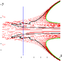
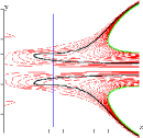
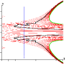
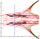
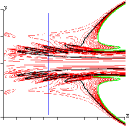
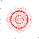
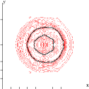
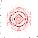
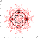
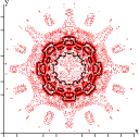
a)                     b)                     c)                     d)                     e)                   f)                     g)                     h)                     i)                     j)

Figure 4: Contour of $\omega_{\theta}$ in $z-y$ with $-2.25<z-z_{c}<-0.75$ and $-0.75<y<0.75$ in a), b), c), d), e), and $x_{y}$ with $-0.5<x<0.5$ and $-0.5<y<0.5$ in f), g), h), i), j), planes at $t=20$ to enlight shape of the spike red lines with $\Delta=0.005$, thick black $\omega_{\theta}=0.05$, thick green $\omega_{\theta}=0.2$, with $n_{p}=16$ and; a,f) $n_{a}=0$, b,g) $n_{a}=1$, c,h) $n_{a}=2$, d,i) $n_{a}=4$ and e,j) $n_{a}=8$.

A substantial smoothing of the contour $\omega_{\theta}=0.05$ appears in figure 4b, that is corroborated by the two quite circular black lines in figure 4g. However, both figures explain that the increased smoothness is also due to the choice to locate the $y-z$ plane at $\theta=\pi/2$ and $\theta=3\pi/2$. Indeed, structures are visible in figure 4g, but these are weak with respect to those forming for $n_{a}>1$. At $n_{a}=2$ four structures form at the center of the spike, that deform the inner $\omega_{\theta}=0.05$ contour pushing it towards the second one. The intensification of the azimuthal vorticity in certain regions and the decrease in others can not be ascribed to the viscous terms in the $\omega_{\theta}$ transport equation. Therefore it should be due to the balance between advection and vortex tilting and stretching. This budget is presented for the $n_{a}=4$ later on, in the spike it has been observed that the convective transport prevails on the other non-linear terms. At $n_{a}=4$ the structures are more complex and figure 4i depicts the oscillations of the black line in figure 4d. The tendency to have in the central region a more circular spike in the azimuthal direction, by increasing $n_{a}$ can be drawn by figure 4j for $n_{a}=8$. On the other hand this figure shows also that large oscillations appear at the edge of the spike. These are attached at the vortex in a complex way as figure 4e demonstrates. From these images it has been decided that the $n_{a}=4$ could be the wave number more appropriate to investigate the response of the Hill vortex to disturbances of different amplitude, described in the next section.

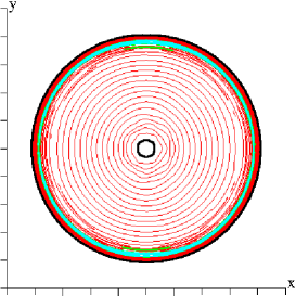
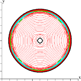
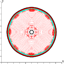
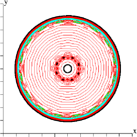
a)                                                b)                                     c)                                                d)

Figure 5: Contour of $\omega_{\theta}$ in a $x-y$ plane and $x_{y}$ with $-1.2<x<1.2$ and $-1.2<y<1.2$ at $t=20$ at $z$ corresponding to the maximum of $<\omega_{\theta}>$ for $\delta_{0}=0.01$: a) $n_{a}=1$, b) $n_{a}=2$, c) $n_{a}=4$ and d) $n_{a}=8$, red contours have an increment $\Delta=.05$ up to $\omega_{\theta}=0.95$, the black thick lines is at $\omega_{\theta}=0.05$, the green at $\omega_{\theta}=1.$ and the cyan have increments $\Delta=.05$ for $\omega_{\theta}>1.$.

The complex physics in the interior of the vortex may reveal important issues during the instability, that my lead to the destruction of the Hill vortex. From figure 3 it may be inferred that the disturbance during the motion is convected in the rear, and is not any more visible in a large part of the surface. The disturbances, at later times, are visible in the complex structures of the spike above described, whose number is strictly connected to the wave number $n_{a}$. We wish to investigate, through visualizations of $\omega_{\theta}$ in $x-y$ planes, whether structures similar to those in the spike are encountered in the central region of the vortex. Figure 5a-d indeed show these structures both near the surface and near the axis. As well as in the spike the number is strictly linked to the azimuthal wave number of the initial perturbation. The common behavior for any wave number $n_{a}$ can be drawn by looking at the time evolution of $\omega_{r}$ and $\omega_{z}$ (not shown for sake of brevity). Up to $t=8$ $\omega_{z}$ grows near the external surface, instead $\omega_{r}$ is concentrated in very thin regions near the axis. These regions grows in time while they move far from the axis. At $t=10$ the size of the $\omega_{r}$ patches are almost equal to those depicted in the central region of figure 5 and to those of $\omega_{z}$ near the surface. At $t=20$, from the saved field, any term in the transport equation of $\omega_{\theta}$ have been evaluated. The equation is

$${{\partial\omega_{\theta}}\over{\partial t}}=-\underbrace{(\frac{u_{\theta}}{r}{{\partial\omega_{\theta}}\over{\partial\theta}}+u_{r}{{\partial\omega_{\theta}}\over{\partial r}}-\frac{u_{r}\omega_{\theta}}{r}+u_{z}{{\partial\omega_{\theta}}\over{\partial z}})}_{C_{\theta}}+\underbrace{\frac{\omega_{\theta}}{r}{{\partial u_{\theta}}\over{\partial\theta}}+\omega_{r}{{\partial u_{\theta}}\over{\partial r}}-\frac{u_{\theta}\omega_{\theta}}{r}+\omega_{z}{{\partial u_{\theta}}\over{\partial z}}}_{S_{\theta}}+\underbrace{\frac{1}{Re}\nabla^{2}\omega_{\theta}}_{V_{\theta}}$$ (5)

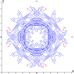
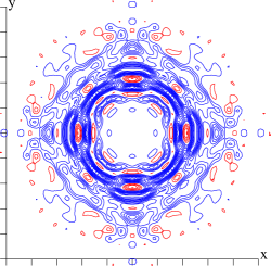
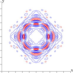
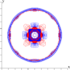
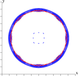
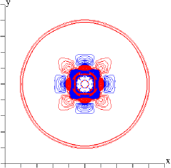
a)                                   b)                                   c)                       d)                                   e)                                   f)

Figure 6: For $n_{a}=4$ disturbance contour plots of the terms in the Eq.(5): top figures at the same $z$ location and $x,y$ limits as in figure 4 with increment $\Delta=.001$ , bottom at the same $z$ and $x,y$ limits as in figure 5 with increment $\Delta=.01$ blue negative, red positive a) and d) $C_{\theta}$, b) and e) $u_{r}{{\partial\omega_{\theta}}\over{\partial r}}-\frac{u_{r}\omega_{\theta}}{r}$ c) and f)$u_{z}{{\partial\omega_{\theta}}\over{\partial z}}$.

The large Reynolds number imply a small effect of the viscous term, then the convective $C_{\theta}$ and the stretching and tilting terms ($S_{\theta}$) should be relevant. Since, the total contribution of $S_{\theta}$ in each location is smaller than that of $C_{\theta}$, the $S_{\theta}$ distribution is not shown. Each term of $C_{\theta}$ contribute at a different rate depending on the region, and in particular, $\frac{u_{\theta}}{r}{{\partial\omega_{\theta}}\over{\partial\theta}}$ is negligible everywhere, therefore this is not presented. The entire $C_{\theta}$ contribution in figure 6a reproduces with a good approximation the $\omega_{\theta}$ contours in figure 4a, in any location is negative and this implies that the strength of the spike is reduced by convection; it becomes longer as it was found by the present results in figure 2c. Looking at each contribution to $C_{\theta}$, $u_{r}{{\partial\omega_{\theta}}\over{\partial r}}-\frac{u_{r}\omega_{\theta}}{r}$ in figure 6b prevails on $u_{z}{{\partial\omega_{\theta}}\over{\partial z}}$ in figure 6c. The latter in certain points is positive, but the opposite action of the former prevails resulting in $C_{\theta}<0$ everywhere. At the center of the vortex the figure 5 shows the accumulation and depletion of $\omega_{\theta}$ near the axis and near the external surface. These correspond to the red and blue regions of $C_{\theta}$ in figure 6d. Figure 6e shows that $u_{r}{{\partial\omega_{\theta}}\over{\partial r}}-\frac{u_{r}\omega_{\theta}}{r}$ is mainly concentrated near the external surface, instead $u_{z}{{\partial\omega_{\theta}}\over{\partial z}}$ acts near the axis, as is seen in figure 6f.

\psfrag{ylab}{$\Delta\omega_{\theta}$}\psfrag{xlab}{ $x$}\includegraphics[width=184.9429pt,clip,angle={0}]{fig7b.eps}

\psfrag{ylab}{$\Delta\omega_{\theta}$}\psfrag{xlab}{ $x$}\psfrag{ylab}{$$}\psfrag{xlab}{ $x$}\includegraphics[width=184.9429pt,clip,angle={0}]{fig7a.eps}

a)                                                       b)

Figure 7: Profiles of $\Delta\omega_{\theta}$ along $x$ at $y=0$ every $4$ time units indicated in the legend, in a) the layer in the left, in b) the layer in the center of figure 5.

From this figure it can be inferred that inside the vortex the $C_{\theta}$ generates waves transferring disturbances from the interior towards the surface. In order to demonstrate that these are true travelling waves the red and blue regions should be concentrate at a certain time in a small region, and later on should move from this to other regions. Instead if these remain fix at a certain location these could be related to insufficient resolution. Indeed it was mentioned that at $Re=60000$ small oscillation remains near the edge of the vortex due to the impossibility to describe the sharp interface. Instead of presenting at each time the distribution of $\omega_{\theta}$ in a $x-y$ plane a simple and more efficient vision can be given by the profiles, at $\theta=0$, of $\Delta\omega_{\theta}=\omega_{\theta}(x,0,t)-\omega_{\theta}(x,0,0)$. Figure 7a confirms that the numerical oscillations near the interface do not grow and do not move far from the region where are produced. On the other hand, the same plot in the central region ($0<x<0.6$) shows that at $t=4$ (green) $\omega_{\theta}$ did not change much and that at $t=8$ (blue) a small undulation starts to grow. At $t=12$ (magenta) the oscillation of reasonable amplitude is depicted and the prof that it is a true wave is given by the peaks shifted on the right with respect to those at $t=8$. The other two profiles at $t>12$ emphasise that the disturbance grow at the center and moves towards the external surface of the vortex. The amplitude of the disturbances are rather small thus it can be concluded that for small disturbances applied on the surface and, after a short translation, the vortex has a perturbed shape not too different from that at $t=0$.

3.4 Effect of the amplitude of the perturbations

In the previous section it has been observed that the azimuthal disturbances are triggering the basic state of the Hill vortex producing in certain regions an increase and in other a decrease of $\omega_{\theta}$. This should be similar to what take place in vortex rings. In this vortex the azimuthal disturbances grow in time, the circular shape is not preserved, and at a certain time the complete destruction of the vortex ring occur. This evolution is clearly described by the pictures at Page 67 of van Dyke (1982). The difference between a ring and the Hill vortex is that the former is not and the latter is a form-preserving solution of the Euler equations. A perfect Hill vortex can not be created in a laboratory, therefore numerical experiments are the only way to investigate whether the Hill behaves as a toroidal ring. From the, above discussed, results in presence of small disturbances it seems that the instability of Hill vortices give rise to a sort of wake but large part of the structure retain its initial $<\omega_{\theta}>$. In two dimensions it has been observed that the Lamb dipole (Lamb (1932)), a form preserving solution of the Euler equations, subjected to strong disturbances leaves behind a wake, proportional to the disturbance, and a new structure with the same characteristic of the original one forms. This has been investigated by Cavazza et al. (1992) by assigning different kind of disturbances, and finally getting a dipole characterised by a linear relationship between vorticity and stream function.

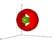
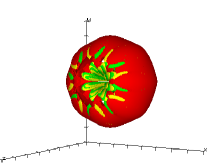
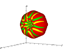
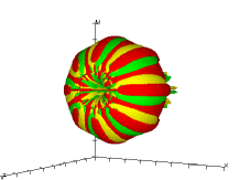
a)                                   b)                                   c)                            d)                                   e)                                   f)

Figure 8: Surface contour of $\omega_{\theta}=0.7$ (red) and $\omega_{z}=\pm 0.1$ positive yellow negative red at $t=20$ for: a) $\delta_{0}=0.01$, b)$\delta_{0}=0.03$, c) $\delta_{0}=0.06$, d) $\delta_{0}=0.09$, e) $\omega_{\theta}=0.7$ (red) and $\omega_{r}=\pm 0.1$ at $t=20$, f) $\omega_{\theta}=0.7$ (red) and $\omega_{z}=\pm 0.1$ at $t=0$

In 2D there is no vortex stretching in the vorticity transport equations. In 3D the vortex stretching and tilting terms are fundamental to go from the laminar through an instability to the turbulent regime. For small disturbances and a short evolution it has been found that the $S_{\theta}$ terms are smaller than $C_{\theta}$. By increasing the amplitude of the disturbance the transition process may be faster, this explains why large disturbances on the surface of the Hill vortex are applied and discussed in this section. At $t=0$ the contour $<\omega_{\theta}>=0.1$ for $\delta_{0}=0.09$ compared to the black line in figure 2b for $\delta_{0}=0.01$ emphasise that a very corrugated surface has been generated. This plot is not presented because the average in $\theta$ reduces the vision of the complexity of the surface, that instead is appreciated by a $\omega_{\theta}=0.7$ contour in figure 10f. It is important to recall that this value is located at a distance from the centre where the $\omega_{\theta}$ sharply goes to zero. To understand the large modifications of the vorticity components while the vortex evolves from $t=0$ up to $t=20$ the surfaces of $\omega_{z}=\pm 0.1$ are superimposed to that of $\omega_{\theta}$ in figure 8f. The effects of the polar and azimuthal disturbances are depicted by small patches of $\omega_{z}$ in the regions of high curvature of $\omega_{\theta}$. The visualizations at $t=20$ allow to understand the dependence of the secondary vorticity on the amplitude of the disturbance, namely are shown for $\delta_{0}=0.01$ in figure 8a, for $\delta_{0}=0.03$ in figure 8b, for $\delta_{0}=0.06$ in figure 8c and for $\delta_{0}=0.09$ in figure 8d. At $t=20$ the polar disturbances are barely visible on the red surface of $\omega_{\theta}=0.7$, these have been convected in the rear side forming the long spike region with a corrugation more complex higher the amplitude of the disturbance. The azimuthal disturbances cause the formation of secondary vorticity components near the axis and near the surface of the vortex. Those near the axis propagate towards the surface, and as can be inferred in figure 8, depending on their magnitude are convected around the front stagnation point and remain close to the external surface of the vortex. In this region the secondary vorticity contributes to the deformation of the surface of the vortex with an amplitude of the azimuthal waviness greater than that at $t=0$. By comparing figure 8d and figure 8e it is rather difficult to establish which component of the two secondary vorticity components prevail to deform $\omega_{\theta}$.

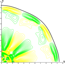
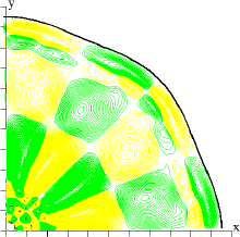
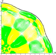
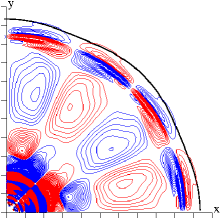
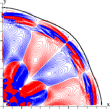
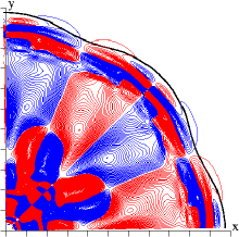
a)                                        b)                                        c)                                       d)                                        e)                                        f)

Figure 9: Surface contour, in one quarter of the domain, of $\omega_{\theta}=0.05$ (black) together with: top $\omega_{z}$ positive red negative blue, bottom $\omega_{r}$ positive green negative yellow at $t=20$ at $z=z_{c}$, with increments $\Delta=.01$ a), d) $\delta_{0}=0.03$, b), e) $\delta_{0}=0.06$, c), f) $\delta_{0}=0.09$.

To see in more detail the connection between the secondary vorticity fields near the axis and near the surface of the Hill vortex, one quarter of the box in a $x-y$ plane at the $z$ location of maximum $<\omega_{\theta}>$ has been considered. Indeed the figure 9 shows the strong connection between the small cylindrical patches at the axis, and the ribbon like structure near the surfaces. Differently than in figure 8 the black line is at a value $\omega_{\theta}=0.05$, that depicts better the deformation of the surface of the vortex for any kind of disturbance assigned. The shape of the secondary vorticity patches near the surface does not depend much on the amplitude of the disturbances. However, at high $\delta_{0}$ small patches of $\omega_{z}$ are responsible of the increase of the deformation of the surface. The patches at an intermediate distance are less intense than those near the axis and therefore the undulations of $\omega_{\theta}$ are smaller than those near the axis , and near the surface. The common features drawn by figure 9 is that the two vorticity components, at this time, are almost equal in the region around the axis, and that by increasing $\delta_{0}$ $\omega_{z}$ affects in a large measure the deformation of external vortex surface.

These simulations, performed in a fixed reference frame, are evolving for $20$ time units, to prevent that the vortex, exiting from the domain, reenters encountering part of the spike. In this lapse of time it has been noticed that the deformation of the surface increase up to $t=6$ and later on does not change up to $t=20$. From this observation it can be concluded that strong disturbances applied to the Hill vortex produce secondary vorticity components ($\omega_{r}$ and $\omega_{z}$) at its interior that grows in amplitude and move towards the external surface. However, the main vortex continues to travel remaining compact without breaking in small scales typical of turbulent flows. This conclusion is questionable since it is based on simulations evolving for a relative short time.

3.5 Frame moving simulations

\psfrag{ylab}{$Q_{i}$}\psfrag{xlab}{ $$}\includegraphics[width=184.9429pt,clip,angle={0}]{fig10a.eps}

\psfrag{ylab}{$Q_{i}$}\psfrag{xlab}{ $$}\psfrag{ylab}{$$}\psfrag{xlab}{ $$}\includegraphics[width=184.9429pt,clip,angle={0}]{fig10c.eps}

a)                                                         b) \psfrag{ylab}{$Q_{i}$}\psfrag{xlab}{ $$}\psfrag{ylab}{$$}\psfrag{xlab}{ $$}\psfrag{ylab}{$\Omega_{i}$}\psfrag{xlab}{ $t$}\includegraphics[width=184.9429pt,clip,angle={0}]{fig10b.eps} \psfrag{ylab}{$Q_{i}$}\psfrag{xlab}{ $$}\psfrag{ylab}{$$}\psfrag{xlab}{ $$}\psfrag{ylab}{$\Omega_{i}$}\psfrag{xlab}{ $t$}\psfrag{ylab}{$$}\psfrag{xlab}{ $t$}\includegraphics[width=184.9429pt,clip,angle={0}]{fig10d.eps}                           c)                                                         d)

Figure 10: Time evolution for $n_{a}=4$ of the velocity $Q_{i}$ for, a) $\delta_{0}=0.01$, b) $\delta_{0}=0.03$ and vorticity $\Omega_{i}$, c) $\delta_{0}=0.01$, d) $\delta_{0}=0.03$; red azimuthal, green radial and blue axial components, lines fixed open symbols moving frame.

To analyse the space evolution of the Hill vortex for long time the computational domain in the streamwise direction should be long enough do not let the vortex to leave the computational box. For instance to travel for $t=100$, that is five time longer than in the previous sections, a greater computational effort is necessary. A more productive way, by using the same length in $z$, consists on solving the Navier-Stokes equations in a reference frame moving with the theoretical velocity $U=-2/15$. The aim of a long evolution is to verify whether the secondary motion becomes strong enough not only to deform the external surface but also to destroy the large scale structure, giving rise to small scales propagating everywhere, that is to produce a fully turbulent flows. The $n_{a}=4$ disturbances have been simulated for $\delta_{0}=0.01$ and $\delta_{0}=0.03$ amplitudes. The former is devoted to investigate whether, for small disturbances, a stop on the growth of the strength of the secondary vorticity components may occur. The latter one produces a faster growth and symmetry breaking. The two cases allow to see whether an universal behaviour can be established. The results of space and time developing simulations should have similar trends. The eventual small differences can be detected by looking at the time evolution of the velocity and vorticity mean square in the whole domain. If $\overline{u_{i}}=<u_{i}>$ and $\overline{\omega_{i}}=<\omega_{i}>$ the mean square are defined as $Q_{i}=\frac{\Sigma_{i}\Sigma_{j}\Sigma_{k}}{N_{1}N_{2}N_{3}}(u_{i}-\overline{u_{i}})^{2}$, $\Omega_{i}=\frac{\Sigma_{i}\Sigma_{j}\Sigma_{k}}{N_{1}N_{2}N_{3}}(\omega_{i}-\overline{\omega_{i}})^{2}$. Figure 10 indeed shows the rather good agreement of the time evolution in the different frame of reference. It is worth to remind that without azimuthal disturbances the mean square are zero. In addition the evolution of $Q_{i}$ (figure 10a and figure 10b) and of $\Omega_{i}$ (figure 10c and figure 10d) demonstrate that, in the first $20$ time units, for low ($\delta_{0}=0.01$) and high ($\delta_{0}=0.03$) amplitude, the evolution of each component has similar trend. However the scale of the coordinates evinces that for $\delta_{0}=0.03$ values almost ten times higher than those for $\delta_{0}=0.01$, implying an eventual scaling with the corresponding values at $t=0$ that are proportional to the amplitude of the disturbance.

\psfrag{ylab}{$K/k_{0}$}\psfrag{xlab}{ $t$}\includegraphics[width=184.9429pt,clip,angle={0}]{fig11a.eps}

\psfrag{ylab}{$K/k_{0}$}\psfrag{xlab}{ $t$}\psfrag{ylab}{$\chi/\chi_{0}$}\psfrag{xlab}{ $t$}\includegraphics[width=184.9429pt,clip,angle={0}]{fig11b.eps}

a)                                                         b)

Figure 11: Time evolution of a) turbulent kinetic energy b) enstrophy scaled by the corresponding values at $t=0$ purple $n_{a}=4$: symbols $\delta_{0}=0.03$, lines $\delta_{0}=0.01$; black random: symbols $\delta_{0}=0.09$,lines $\delta_{0}=0.01$; inset in a) mean square velocity components scaled by $Q_{z}(t=0)$, red $Q_{\theta}$, green $Q_{r}$, blue $Q_{z}$ left $n_{a}=4$ right random the same colours and symbols for b).

The aim of the DNS is to investigate whether the Hill vortex, while is travelling for a long distance, maintains a shape similar to the initial one or instead is disrupted. In addition, it was noticed that, in a short interval of time, the azimuthal symmetry is preserved, implying that, the small round-off errors are not amplified by the growth of secondary vorticity. We wish to point out that, on purpose, single precision has been used to verify for how long the symmetry is preserved. To enhance the destruction of the Hill vortex large amplitude disturbances ($\delta_{0}=0.09$ and $\delta_{0}=0.03$) with a random distribution of azimuthal wave numbers have been introduced at $t=0$. The profiles of the total turbulent kinetic energy $K=\Sigma Q_{i}$ and the enstrophy $\chi=\Sigma\Omega_{i}$ versus time, in figure 11a and figure 11b, give a first impression of the influence of the disturbance on a long time evolution. To investigate the dependence on the amplitude and on the number of the number $n_{a}$ of waves excited, $K$ and $\chi$ have been scaled with their values at $t=0$ ($K_{0}$ and $\chi_{0}$). The figures show that an independence on the amplitude of the disturbance does exist, in fact, in both the figures 11 the profiles of the lines (small amplitude) and of the symbols (large amplitude) are almost coincident. On the other hand, the trend of the random wave number disturbances differs from that for $n_{a}=4$. Similarity and differences can be appreciated also for each mean square component, as it is shown in the insets of figure 11. When a single wave number is excited the initial radial and axial velocity mean square components remain constant for few time units, while the azimuthal components grows exponentially. Later on all three $Q_{i}$ components grow up to $t=60$ (figure 11a) for both amplitudes, as it is enlightened by the coincidence of the purple line and symbols. For $t>60$ the two curves diverge. Flow visualizations in orthogonal planes to the $z$ axis allow to understand the reasons of this separation. For random disturbances the time history is independent on $\delta_{0}$. The initial decrease of $K$ can be ascribed to the transfer of energy among scales due to the different energy level for each wave number at $t=0$. Figure 11b shows for $\chi/\chi_{0}$ a trend similar to that of $K/K_{0}$, with a drop in the first time units greater than that for $K/K_{0}$. In addition for a single wave number excitation the trends of each component of $\chi/\chi_{0}$ differ from those with disturbances at random wave number. In the former case at $t=0$ the amount of $\Omega_{z}$ is rather small, through a fast growth it reaches the level of the others, and all three continue to grow. The growth for $t>30$ implies an enhancement of the vorticity components in well localised regions as it is corroborated by visualizations. The inset relative to the random disturbances has still a constant evolution in the first few time units with a greater $\Omega_{z}$ than that for $n_{a}=4$. The interesting result is that during the fast growth for $t>30$ all three reach values $O(1)$, while for $n_{a}=4$ a level $O(100)$ is reached. For $t>55$ $K/K_{0}$, in the case of $n_{a}=4$, show a different trend for $\delta_{0}=0.01$ (lines) and for $\delta_{0}=0.03$ (symbols) due to the symmetry persistence for the former, implying vorticity components very intense in localised small regions. On the other hand, for the $\delta_{0}=0.03$ the symmetry is lost at $t\approx 55$ and the growth of $K/K_{0}$ reduces and becomes closer to that for random disturbances.

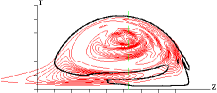
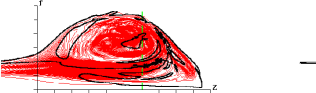
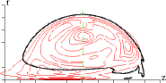
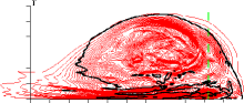
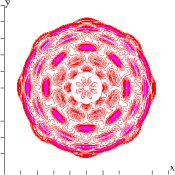
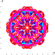
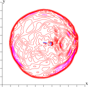
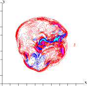
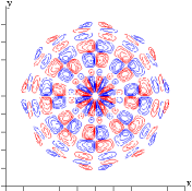
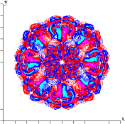
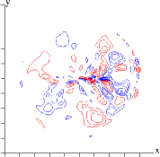
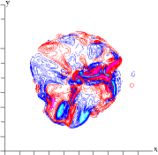
a)                           b)                           c)                           d)                      e)                           f)                           g)                           h)                      i)                           j)                           k)                           l)

Figure 12: Contours at $t=60$ of $\Sigma<u_{i}^{2}>$ (red $\Delta=.00005$) superimposed to $<\omega_{\theta}>=0.1$ black, for $-1.75<z-z_{c}<0.75$ and $0<r<1.2$: in a) $n_{a}=4,\delta_{0}=0.01$, b) $n_{a}=4,\delta_{0}=0.03$ , c) random $\delta_{0}=0.03$, d) random $\delta_{0}=0.09$; the green lines correspond to the location where the $\omega_{\theta}$ and $\omega_{r}$ contours ($-1.2<x<1.2$ ,$-1.2<y<1.2$) in e,i) as a), f,j) as b), g,k) as c) and h,l) as d) ; $\Delta=0.1$ red up to $\omega_{\theta}<1$, magenta $\omega_{\theta}>1.$, black $\omega_{\theta}=1$; $\Delta=-0.1$ blue for $\omega_{\theta}<0$, cyan for $\omega_{\theta}<-1$.

To understand better the above discussion on the time behaviour of $K$ and $\chi$ that are linked to the generation of a hierarchy of vortical structures is worth looking to the vorticity field, directly connected to the flow structures. In the top panels of figure 12 the contours of $<\omega_{\theta}>=0.1$ (black line) demonstrate that, the Hill vortex strongly perturbed with $n_{a}=4$ does not survive for a long time. In fact its characteristic shape at $t=60$ is destroyed in the inner region. This modification is more visible in figure 12b than in figure 12a. In correspondence to the large undulation of $<\omega_{\theta}>=0.1$, at a distance $r=0.2$ from the axis the fluctuating kinetic energy (the red contours) is large (figure 12a) and increases in figure 12b. The increase for $\delta_{0}=0.03$ of the velocity fluctuations produces a large deformation of $<\omega_{\theta}>$ in the interior of the vortex and in a greater measure near the front. To understand the flow structures at the interior of the vortex visualizations of the vorticity components in $x-y$ planes at the streamwise location of the maximum of $<\omega_{\theta}>$ may help. The magenta patches in figure 12e indicate regions with $\omega_{\theta}>1$, implying that the circular distribution of $\omega_{\theta}$ at $t=0$ and of the similar one at $t=20$ (figure 5a) is destroyed at $t=60$. This excess of vorticity is generated by the convective and stretching terms in Eq.(5). It has been observed, that also at $t=60$ $C_{\theta}$ prevails on $S_{\theta}$. For $\delta_{0}=0.01$ there is a reduction of the distance between the contour lines of $<\omega_{\theta}>$ in a $r-z$ plane, from $r=0$ up to the center of the vortex. The thickness of these layers is close to that in figure 12e. On the other hand, from the center to the external surface of the vortex the separation of the contours is close to that at $t=0$. For $n_{a}=4$ and $\delta_{0}=0.03$ even the regions near the surface present intensification in certain layers, and, in particular, near the front. This intensification can be understood by the $\omega_{\theta}$ visualization in figure 12f that enlight the formation of $\omega_{\theta}<0$ (blue lines) in certain regions close to other with $\omega_{\theta}<-1$ (cyan lines). Close to these patches there are other location with $\omega_{\theta}>1$. This condition with high vorticity gradients is very unstable. High gradients of all the vorticity components are produced as it is shown by the contours of $\omega_{r}$ in figure 12j. The figure of $\omega_{z}$ (not shown), similar to that of $\omega_{r}$ and of $\omega_{\theta}$, demonstrate that inside the vortex the secondary motion is comparable to the primary one. In these two figures it can be appreciated that the symmetry is no longer good as that for $\delta_{0}=0.01$. Later on the vorticity field is similar to that produced by random disturbances. The difference is that for $t>60$ and for $n_{a}=4$ in figure 11 the values of $K$ and $\chi$ are greater than those for random disturbances, and as a consequence the initial structure of the vortex is no longer recognisable. By random disturbances with amplitude $\delta_{0}=0.03$ the growth of secondary vorticity is reduced (figure 11) and the vorticity field is not concentrated in localised structures (figure 12g and figure 12k). The low level of $K$ in figure 11a is corroborated by the reduced number of contours in figure 12c and that of $\chi$ in figure 11b by their reduction in figure 12g and figure 12k. Figure 12c shows, through the contour of $<\omega_{\theta}>=0.1$, an external boundary without a wake and with a shape similar to that at $t=0$. However the convoluted contours of $\omega_{\theta}$ at the interior (figure 12g) are very different from the circular one at $t=0$. By random disturbances with $\delta_{0}=0.09$ the corresponding figures, figure 12d,figure 12h and figure 12l demonstrate that at the interior is rather difficult to recognise any structure typical of the Hill vortex.

4 Conclusions

Direct numerical simulations of the Navier-Stokes equations have been performed to investigate whether the results, obtained by simplified equations, on the instability of Hill vortices are reproduced by the real conditions with a small amount of viscosity. Indeed, it has been observed that by imposing polar disturbances on the surfaces a tail on the rear of the vortex forms. At high Reynolds number the elongation of the spike agrees with that predicted by the simplified Euler equations. During the evolution the polar disturbances are convected in the wake and large part of the vortex surface has a shape similar to the initial one. The two convective terms in the transport equation of $\omega_{\theta}$ are mainly localised near the surface, with that due to $u_{r}$ greater than that due to $u_{z}$. In the interior of the vortex the convective terms are zero implying that the initial vorticity does not change. From these axisymmetric simulations it may be inferred that the Hill vortex behaves as the Lamb dipole in two-dimensions, that is, both shed an amount vorticity in a wake and, with exception of a thin layer near the boundary the vorticity distribution in the central region do not change. By adding to the polar azimuthal disturbances on the surfaces we are in presence of three-dimensional flows, that is characterised by the growth of a secondary motion. Even the three-dimensional disturbances are convected far from the surfaces and accordingly the structure of the spike in the rear is modified. The DNS allows to follow the growth of the secondary motion through visualizations of the vorticity field at the interior of the vortex. The disturbances on the surface induce, as it is expected, a weak secondary vorticity nearby, that does not largely increase in time. On the other hand, a strong secondary vorticity field is generated near the axis. These act as travelling waves growing in amplitude and moving towards the surface. By increasing the amplitude of the disturbance the evolution is faster, but it has been observed that for Hill vortices travelling for a short distance the vortex is not destroyed, that is does not create a hierarchy of large and small scale structures typical of turbulent flows. The transition from ordered to disordered structures is due to the action of the several terms in the vorticity transport equations. The evaluation of all the non-linear terms in the transport equation of the primary azimuthal vorticity has shown that the convective terms prevail on the vortex stretching and tilting. The effect of the latter increases with the amplitude of the disturbance.

The conclusion drawn by short time simulation have a relative validity, to be more convincing should be based on simulations lasting for a long time. These are inefficient, from computational aspects in a fixed reference frame. The simulations were repeated in a reference frame moving with the theoretical translational speed of the Hill vortex. In these circumstances it has been found that the vortex perturbed by three-dimensional disturbances at a fixed and at several wave numbers randomly chosen leads to situation that at later time give rise to the complete destruction of the vortex. At the very large Reynolds number here chosen to be as much as possible close to the Euler equations, the growth of the secondary vorticity components is high and the kinetic energy associated with them is not dissipated. The velocity components in certain small regions become very large and the numerical stability restrictions on the $\Delta t$, due to the explicit treatment of the non-linear terms, limit the time of the simulations. A first estimate of a Taylor microscale Reynolds number give values order $200$ and to see how far we are from a turbulent flows spectra in the homogeneous direction should be evaluated. This will investigated in the near future at low Reynolds numbers.

5 Acknowledgments

This work was inspired by a discussion with Keith Moffat during his visit in Roma approximately 10 years ago. The authors wish to thank Sergio Pirozzoli and George Carnevale for the fruitful discussions. We acknowledge that some of the results reported in this paper have been achieved using the PRACE Research Infrastructure resource GALILEO based at CINECA, Casalecchio di Reno, Italy.

References

- Cavazza et al. (1992) Cavazza, P., van, G.J.F. Heijst & Orlandi, P. 1992 The stability of vortex dipoles. Proceedings of the 11th Australasian Fluid Mech. Conf., Hobart, Australia p. 67.
- Crow (1970) Crow, S.C. 1970 Stability theory for a pair of trailing vortices. AIAA J. 8, 2172–2179.
- van Dyke (1982) van Dyke, M. 1982 An album of fluid motion. The Parabolic Press, Satnford Ca.
- Fukuyu et al. (1994) Fukuyu, A., Ruzi, T. & Kanai, A. 1994 The response of hill’s vortex to a small three dimensional disturbance. J. Phys. Soc. Japan 63,, 510–527.
- Hill (1894) Hill, M.J.M. 1894 On a spherical vortex. Phil. Trans. R. Soc. Lond. A 185, 213–245.
- Lamb (1932) Lamb, H. 1932 Hydrodynamics. Cambridge University Press.
- Leweke & Williamson (1998) Leweke, T. & Williamson, C.H.K. 1998 Cooperative elliptic instability of a vortex pair. J. Fluid Mech. 360, 85–119.
- Melander et al. (1987) Melander, M. V., McWilliams, J.C. & Zabusky, N.J. 1987 Axisymmetrization and vorticity gradient intensification of an isolated two-dimensional vortex through filamentation. J.Fluid Mech. pp. 137–159.
- Moffat & Moore (1978) Moffat, H.K. & Moore, D.W. 1978 The response of hill’s spherical vortex to a small axisymmetric disturbance. J. Fluid Mech. 87, 749–760.
- Orlandi (2000) Orlandi, P. 2000 Fluid fow phenomena: a numerical toolkit. Kluwer.
- Orlandi et al. (2001) Orlandi, P., Carnevale, G. F., Lele, S.K & Shariff, K. 2001 Thermal perturbation of trailing vortices. Eur. J. Mech. B - Fluids 20, 511–524.
- Orlandi & Fatica (1997) Orlandi, P. & Fatica, M. 1997 Direct simulations of a turbulent pipe rotating along the axis. J. Fluid Mech. 343, 43–72.
- Orlandi et al. (2012) Orlandi, P., Pirozzoli, S. & Carnevale, G.F. 2012 Vortex events in euler and navierstokes simulations with smooth initial conditions. J. Fluid Mech. 690, 288–320.
- Orlandi & Verzicco (1993) Orlandi, P. & Verzicco, R. 1993 Vortex ring impinging on a wall: axisymmetric and three-dimensional simulations. J. Fluid Mech 256, 615–645.
- Pozrikidis (1986) Pozrikidis, C. 1986 The nonlinear instability of hill’s vortex. J. Fluid Mech. 168, 337–367.
- Protas & Elcrat (2016) Protas, B. & Elcrat, A. 2016 Linear stability of hill’s vortex to axisymmetric perturbations. J. Fluid Mech 799, 579–60.
- Ren & Lu (2015) Ren, Heng & Lu, Xi-Yun 2015 Dynamics and instability of a vortex ring impinging on a wall. Commun. Comput. Phys. 18, 1122–1146.
- Rozi (1999) Rozi, T. 1999 Evolution of the surface of hill’s vortex subjected to a small three-dimensional disturbance for the cases of m = 0, 2, 3 and 4. J. Phys. Soc. Japan 68, 2940.
- Shariff et al. (1994) Shariff, K., Verzicco, R. & Orlandi, P. 1994 A numerical study of three-dimensional vortex ring instabilities: viscous corrections and early non-linear stage. J. Fluid Mech. 279, 351–374.
- Stanaway et al. (1988) Stanaway, S., Shariff, K. & Hussain, F. 1988 Head-on collision of viscous vortex rings. Proceedings of CTR summer school 1988 .
- Verzicco & Orlandi (1996) Verzicco, R. & Orlandi, P. 1996 A finite difference scheme for direct simulation in cylindrical coordinates. J. Comp. Phys. 123, 402–414.
- Widnall et al. (1974) Widnall, S.E., Bliss, D.B. & Tsai, C.-Y. 1974 The instability of short waves on a vortex ring. J. Fluid Mech. 66, 35–47.
- Wray (1987) Wray, A.A 1987 Very low storage time-advancement schemes. Internal Report, NASA Ames Research Center, Moffett Field, California .