Revealing the Phase Diagram of Kitaev Materials by Machine Learning:
Cooperation and Competition between Spin Liquids

Abstract

Kitaev materials are promising materials for hosting quantum spin liquids and investigating the interplay of topological and symmetry-breaking phases. We use an unsupervised and interpretable machine-learning method, the tensorial-kernel support vector machine, to study the honeycomb Kitaev-$\Gamma$ model in a magnetic field. Our machine learns the global classical phase diagram and the associated analytical order parameters, including several distinct spin liquids, two exotic $S_{3}$ magnets, and two modulated $S_{3}\times Z_{3}$ magnets. We find that the extension of Kitaev spin liquids and a field-induced suppression of magnetic order already occur in the large-$S$ limit, implying that critical parts of the physics of Kitaev materials can be understood at the classical level. Moreover, the two $S_{3}\times Z_{3}$ orders are induced by competition between Kitaev and $\Gamma$ spin liquids and feature a different type of spin-lattice entangled modulation, which requires a matrix description instead of scalar phase factors. Our work provides a direct instance of a machine detecting new phases and paves the way towards the development of automated tools to explore unsolved problems in many-body physics.

I Introduction

Kitaev materials have attracted immense attention in the search for quantum Kitaev spin liquids (KSLs) Kitaev (2006). These materials feature highly anisotropic magnetic interactions, a necessary ingredient to realize the Kitaev model, and are found in Mott insulators with strong spin-orbit coupling Jackeli and Khaliullin (2009); Chaloupka et al. (2010); Takagi et al. (2019); Winter et al. (2017a). Experimental signatures of the half-quantized thermal Hall effect, a key characteristic of spin-$1/2$ KSLs, in $\alpha$-$\mathrm{RuCl}_{3}$ Kasahara et al. (2018); Yokoi et al. (2020), and the absence of noticeable magnetic orders in ${\rm H_{3}LiIr_{2}O_{6}}$ Kitagawa et al. (2018) and ${\rm Cu_{2}IrO_{3}}$ Takahashi et al. (2019) demonstrate that these materials are considered among the most prominent candidates for hosting spin liquids. Theoretical studies have put forward an even greater variety of spin liquids and other exotic states Song et al. (2016); Kimchi and You (2011); Singh et al. (2012); Price and Perkins (2012); Li et al. (2015); Sears et al. (2015); Janssen et al. (2016, 2017); Jiang et al. (2019); Chern et al. (2020); Gordon et al. (2019); Wang et al. (2019); Lee et al. (2020); Gohlke et al. (2018, 2020); Osorio Iregui et al. (2014); Gohlke et al. (2017); Motome and Nasu (2020); Zhu et al. (2018); Hickey and Trebst (2019); Hickey et al. (2020); Zhu et al. (2020); Don (2020); Berke et al. (2020); Khait et al. (2020); Rousochatzakis et al. (2015) and generalized the family of Kitaev materials to high-spin systems Stavropoulos et al. (2019); Xu et al. (2020). Three-dimensional hyper- and stripy-honeycomb materials are also synthesized in iridates $\beta$-, $\gamma$-${\rm Li}_{2}{\rm IrO}_{3}$ and are and under active investigation Takagi et al. (2019); Modic et al. (2014); Takayama et al. (2015); Biffin et al. (2014); Ruiz et al. . Nevertheless, this enormous progress goes hand in hand with many open questions. The role of non-Kitaev interactions, which generically exist in real materials, is yet to be understood. The microscopic model of prime candidate compounds including $\alpha$-$\mathrm{RuCl}_{3}$ and the nature of their low-temperature phases remain under debate Kim et al. (2015); Kim and Kee (2016); Winter et al. (2016); Yadav et al. (2016); Ran et al. (2017); Hou et al. (2017); Winter et al. (2017b); Eichstaedt et al. (2019); Sears et al. (2020); Banerjee et al. (2017, 2016); Koitzsch et al. (2017); Majumder et al. (2015); Johnson et al. (2015); Cao et al. (2016); Lampen-Kelley et al. (2018a); Balz et al. (2019); Gass et al. (2020); Wang et al. (2017); Banerjee et al. (2018); Wolter et al. (2017); Lampen-Kelley et al. (2018b); Laurell and Okamoto (2020); Maksimov and Chernyshev (2020); Bachus et al. (2020). Moreover, conceptual understanding beyond the exactly solvable Kitaev limit largely relies on mean-field and spin-wave methods Rau et al. (2014, 2016); Chaloupka and Khaliullin (2015); Rusnačko et al. (2019); Janssen and Vojta (2019); Okamoto (2013), as different numerical calculations of the same model Hamiltonian predict phase diagrams that are qualitatively in conflict with each other Jiang et al. (2019); Wang et al. (2019); Gordon et al. (2019); Lee et al. (2020); Chern et al. (2020); Gohlke et al. (2018, 2020).

A data-driven approach such as machine learning may open an alternate route to research in Kitaev materials. In recent years, its potential in physics has begun to be realized Carleo et al. (2019); Carrasquilla (2020). Successful applications include representing quantum wave functions Carleo and Troyer (2017), learning order parameters Ponte and Melko (2017); Wang (2016), classifying phases Carrasquilla and Melko (2017); van Nieuwenburg et al. (2017), designing algorithms Liao et al. (2019); Liu et al. (2017), analyzing experiments Nussinov et al. (2016); Zhang et al. (2019) and optimizing material searches Schmidt et al. (2019). Most of these advances are focused on algorithmic developments and resolving known problems. Instead, it remains very rare that such techniques are applied to a hard, unsolved problem in physics and provide new insights.

In this article, we employ our recently developed tensorial kernel support vector machine (TK-SVM) Greitemann et al. (2019a); Liu et al. (2019); Greitemann et al. (2019b) to learn the global phase diagram of the honeycomb Kitaev-$\Gamma$ model under a $[111]$ field, which remains unsettled even in the (semi-)classical large-$S$ case. The symmetric off-diagonal $\Gamma$ term is a typical non-Kitaev exchange present in real compounds and can originate from the direct overlap of $d$ orbitals and intermediate $d$-$p$ hopping Rau et al. (2014); Winter et al. (2017b). In particular, in $\alpha$-$\mathrm{RuCl}_{3}$ this exchange is believed to be comparable to the Kitaev interaction Ran et al. (2017); Kim and Kee (2016); Yadav et al. (2016); Winter et al. (2016); Wang et al. (2017). Furthermore, it leads to macroscopic degeneracies and classical spin liquids Rousochatzakis and Perkins (2017).

We determine the global classical phase diagram of the $K$-$\Gamma$-$h$ model in a completely unsupervised fashion. The strong interpretability of TK-SVM further allows us to achieve an analytical characterization of all phases. We hence provide a direct instance of a machine identifying new phases of matter in strongly-correlated condensed matter physics and show that the competition and cooperation between Kitaev and $\Gamma$ spin liquids are key in understanding the emergence of orders in the $K$-$\Gamma$ model. We summarize our main findings below.

First, KSLs can survive non-Kitaev interactions in the large-$S$ limit. The classical phase diagram shows remarkable similarities to its quantum counterpart in the subregion intensively investigated for spin-$1/2$ systems, including a field-induced suppression of magnetic order. Second, the explicit emergent local constraints for classical $\Gamma$ spin liquids ($\Gamma$SLs) are found, and their local transformations are formulated. Third, cooperation and competition between Kitaev and $\Gamma$ constraints lead to two $S_{3}$ orders and two $S_{3}\times Z_{3}$ orders. The latter features a different spin-lattice entangled modulation and may be realized by materials governed by strong Kitaev and $\Gamma$ interactions.

This article is organized as follows. In Section II we define the $K$-$\Gamma$-$h$ Hamiltonian and explain the essential ingredients of TK-SVM. Section III is devoted to an overview of the machine-learned phase diagram. Section IV discusses the emergent local constraints of classical Kitaev and $\Gamma$ spin liquids and their local $Z_{2}$ symmetries. The exotic $S_{3}$ and $S_{3}\times Z_{3}$ orders are elaborated in Section V. We conclude with an outlook in Section VI.

II Model and method

We subject the honeycomb Kitaev-$\Gamma$ model in a uniform $[111]$ field to the analysis of TK-SVM. The spins will be treated as classical $O(3)$ vectors to achieve a large system size which is important to capture competing orders induced by the $\Gamma$ interaction.

Hamiltonian. The $K$-$\Gamma$-$h$ Hamiltonian is defined as

$$H=\sum_{\langle ij\rangle_{\gamma}}\big{[}KS_{i}^{\gamma}S_{j}^{\gamma}+\Gamma(S_{i}^{\alpha}S_{j}^{\beta}+S_{i}^{\beta}S_{j}^{\alpha})\big{]}-\sum_{i}\vec{h}\cdot\vec{S}_{i},$$ (1)

where $K$ and $\Gamma$ denote the strength of Kitaev and off-diagonal interactions, respectively; $\gamma\in\{x,y,z\}$ labels the three different nearest-neighbor (NN) bonds $\langle ij\rangle_{\gamma}$; $\alpha,\beta,\gamma$ are mutually orthogonal; and $\vec{h}=h(1\ 1\ 1)/\sqrt{3}$. We parametrize the interactions as $K=\sin{\theta}$, $\Gamma=\cos{\theta}$, with $\theta\in[0,2\pi)$. The region $\theta\geq 3\pi/2$ corresponds to parameters of $4d$/$5d$ transition metals with ferromagnetic (FM) $K$ Takagi et al. (2019), while $\theta\in[\pi/2,\pi)$ relates to $4f$-electron based systems with anti-ferromagnetic (AFM) $K$ Jang et al. (2019).

The Hamiltonian given by Eq. (1) features a global $C_{6}^{R}C_{3}^{S}$ symmetry which acts simultaneously on the real and spin space, where $C_{6}^{R}$ rotates the six spins on a hexagon (anti-)clockwise, and $C_{3}^{S}$ (anti-)cyclically permutates $\{S^{x},S^{y},S^{z}\}$. In the absence of magnetic fields, the Hamiltonian is also symmetric under a sublattice transformation by sending $K\rightarrow-K$, $\Gamma\rightarrow-\Gamma$, and meanwhile $S_{i}\rightarrow-S_{i}$ for either of the honeycomb sublattices. This sublattice symmetry indicates equivalence between the $K$-$\Gamma$ model of FM and AFM Kitaev interaction, which is respected by the $h=0$ phase diagram shown in Figure 1 (a) and the associated order parameters.

Machine learning. The TK-SVM is defined by the decision function

$$d(\mathbf{x})=\sum_{\mu\nu}C_{\mu\nu}\phi_{\mu}(\mathbf{x})\phi_{\nu}(\mathbf{x})-\rho.$$ (2)

Here, $\mathbf{x}=\{S_{i}^{x},S_{i}^{y},S_{i}^{z}|i=1,2,\dots,N\}$ denotes a spin configuration of $N$ spins, which is the only required input. No prior knowledge of the phase diagram is required.

$\bm{\phi}(\mathbf{x})$ denotes a feature vector mapping $\mathbf{x}$ to an auxiliary feature space. When orders are detected, they are encoded in the coefficient matrix $\mathbb{C}=\{C_{\mu\nu}\}$. The first term in $d(\mathbf{x})$ captures both the form and the magnitude of orders in the system, regardless of whether they are unconventional magnets, hidden nematics Greitemann et al. (2019a); Liu et al. (2019) or classical spin liquids Greitemann et al. (2019b). The extraction of analytical order parameters is straightforward in virtue of the strong interpretability of SVM (see Appendix A for details).

The second term $\rho$ in the decision function is a bias parameter and reflects an order-disorder hierarchy between two sample sets. It detects whether samples in one training set are more ordered or disordered than those in the other set, hence allows one to infer if two states belong to the same phase Liu et al. (2019); Greitemann et al. (2019b). This property of the $\rho$ parameter leads to a graph analysis. By treating points in the physical parameter space as vertices and assigning an edge to any two vertices, one can create a graph with the edge weights determined by $\rho$. Computing the phase diagram is then realized by an unsupervised graph partitioning (see Appendix B).

The concrete application of TK-SVM consists of several steps. First, we collect samples from the parameter space of interest. For the $K$-$\Gamma$-$h$ model, large-scale parallel-tempering Monte Carlo simulations Hukushima and Nemoto (1996); Landau and Binder (2005) are utilized to generate those configurations, with system sizes up to $N=10,\!368$ spins ($72\times 72$ honeycomb unit cells). As major parts of the phase diagram are unknown, we distribute the phase points (almost) uniformly in the $\theta$-$h$ space. In total, $M=1,\!250$ distinct $(\theta,h)$-points at low temperature $T=10^{-3}\sqrt{K^{2}+\Gamma^{2}}$ are collected; each has $500$ sufficiently uncorrelated samples. Then, we perform a SVM multi-classification on the sampled data. From the obtained $\rho$’s, we build a graph of $M$ vertices and $M(M-1)/2$ edges and partition it by Fiedler’s theory of spectral clustering Fiedler (1973, 1975). The outcome is the so-called Fiedler vector reflecting clustering of the graph, which plays the role of the phase diagram [see Figure 1 (c)]. In the next step, based on the learned phase diagram, we collect more samples (typically a few thousands) for each phase and perform a separate multiclassification. The goal here is to learn the $C_{\mu\nu}$ matrices of high quality in order to extract analytical quantities. The dimension of this reduced classification problem depends on the number of phases (subgraphs). Finally, we measure the learned quantities to validate that they are indeed the correct order parameters.

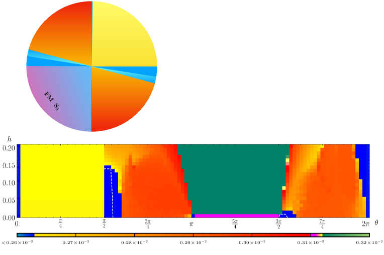
Figure 1: Machine-learned phase diagram for the honeycomb $K$-$\Gamma$ model in a $[111]$ magnetic field, with $K=\sin\theta,\Gamma=\cos\theta$ and at temperature $T=10^{-3}\sqrt{K^{2}+\Gamma^{2}}$. (a) Circular representation of the $h=0$ phase diagram as a function of angle $\theta$. Classical $\Gamma$ ($\Gamma$SLs) and Kitaev (KSLs) spin liquids reside in the limits $\theta\in\{0,\frac{\pi}{2},\pi,\frac{3\pi}{2}\}$ [$(K,\Gamma)=(0,\pm 1),(\pm 1,0)$]. These special limits divide the phase diagram into two frustrated ($K\Gamma<0$) and two unfrustrated ($K\Gamma>0$) regions, labeled by “$-$” and “$+$’, respectively. While $\Gamma$SLs exist only in the two large $\Gamma$ limits, KSLs extend into the frustrated regions, until $|\Gamma/K|_{1}\sim 0.16$ ($\theta\sim 0.551\pi,1.551\pi$). From $|\Gamma/K|_{2}\sim 0.27$ ($\theta\sim 0.584\pi,1.584\pi$), two modulated $S_{3}\times Z_{3}$ orders will be stabilized owing to competition between a KSL and a $\Gamma$SL. These orders have a highly exquisite magnetic structure featuring spin-lattice entangled modulation. In the windows between KSLs and the modulated $S_{3}\times Z_{3}$ orders, there are two non-Kitaev correlated paramagnets (CPs). The two unfrustrated regions respectively host a ferromagnetic (FM) and an antiferromagnetic (AFM) $S_{3}$ order, induced by cooperation between KSLs and $\Gamma$SLs. The $h=0$ phase diagram is symmetric under $\theta\rightarrow\theta+\pi$ and a sublattice transformation (see Section II). (b) Magnetic cells of the $S_{3}$ and modulated $S_{3}\times Z_{3}$ orders. The shaded sites show a magnetic cell for the FM and AFM $S_{3}$ order, comprised of six spins. The modulated $S_{3}\times Z_{3}$ orders consist of three distinct $S_{3}$ sectors (labeled by $A,B,C$) and in total eighteen sublattices (Section V). (c) Finite $h$ phase diagram. The FM $S_{3}$ and the KSL ($\Gamma$SL) for $K=-1$ ($\Gamma=-1$) will be fully polarized (FP) once the $[111]$ field is applied. However, an antiferromagnetic $\Gamma$ extends the FM KSL to a small, but finite, $h\sim 0.01$. AFM $\Gamma$SL and AFM KSL are robust against external fields. The former persists until $h\geq 0.2$, while the latter is non-trivially polarized from $h\sim 0.14$ with global $U(1)$-symmetric correlations [$U(1)_{g}$]. In the frustrated regions and intermediate fields, there are areas of different partially-polarized correlated paramagnets (${\rm CP_{h}}$s). In particular, in the sector of $K<0,\Gamma>0$, the ${\rm CP_{hK^{-}}}$ and ${\rm CP_{h\Gamma^{+}}}$ regimes erode the modulated $(S_{3}\times Z_{3})_{2}$ phase, as field-induced suppression of magnetic order takes hold. Each pixel in the phase diagram represents a $(\theta,h)$ point and is color-coded by the corresponding Fiedler vector entry. The sharp jumps in color coincide with the well-separated peaks in the distribution of Fiedler vector entries, while gentle gradients are indicative of crossovers; cf. Appendix B. Dashed lines separate a spin liquid from a correlated paramagnet, based on susceptibility of the associated ground state constraint (GSC). The Fiedler vector and the GSCs are computed from rank-$1$ and rank-$2$ TK-SVM, respectively. See the text and Appendix B, Appendix C for details.

III Global view of the phase diagram

The $K$-$\Gamma$-$h$ model shows a rich phase diagram, including a variety of classical spin liquids and exotic magnetic orders. In the vicinity of the ferromagnetic Kitaev limit with $\Gamma\gtrsim 0$ (i.e. $\theta\gtrsim\frac{3\pi}{2}$), which has been intensively studied for spin-$1/2$ systems, the classical phase diagram shares a number of important features with the quantum counterpart. We will focus here on the topology of the machine-learned phase diagram. The specific properties of each phase are analyzed in subsequent sections.

We first discuss the phase diagram at $h=0$, depicted in Figure 1 (a). In the absence of external fields the Hamiltonian Eq. (1) has four limits at $(K,\Gamma)=(\pm 1,0)$ and $(0,\pm 1)$, corresponding to two classical KSLs and two $\Gamma$SLs. These particular limits divide the $K$-$\Gamma$ phase diagram into four regions. When both the Kitaev and $\Gamma$ interactions are ferromagnetic or antiferromagnetic, the system is unfrustrated, while when they are of different sign, the system stays highly frustrated.

In the two unfrustrated $K\Gamma>0$ regions, when $K$ and $\Gamma$ are both finite, the system immediately changes from a spin liquid to a magnetic order, which is sometimes described as a $120^{\circ}$ state Rau et al. (2014); Chaloupka and Khaliullin (2015). The explicit order parameter of the two phases corresponds to the symmetric group $S_{3}$, hence we refer to them as the FM $S_{3}$ and AFM $S_{3}$ phase, respectively, to distinguish them from other types of $120^{\circ}$ states. As we shall see in Section V, these two orders can be understood as the result of cooperation between the Kitaev and $\Gamma$ spin liquids.

The physics is profoundly different in the frustrated regions. The two KSLs can extend to a finite value of $\Gamma$ for $K\Gamma<0$. There has been mounting evidence suggesting that quantum KSLs survive in some non-Kitaev interactions Kasahara et al. (2018); Yokoi et al. (2020); Gohlke et al. (2018, 2020); Lee et al. (2020); Wang et al. (2019); Gordon et al. (2019); Osorio Iregui et al. (2014); Gohlke et al. (2017). It is quite remarkable that such an extension already manifests itself in the classical large-$S$ limit. Using the corresponding ground state constraint (GSC), we estimate $|\Gamma/K|\sim 0.16$ (see Appendix C). This large extension may find its origin in the large extensive ground-state degeneracy (exGSD) of classical KSLs.

By contrast, the two classical $\Gamma$SLs are found to only exist in the limit $\Gamma=\pm 1$, as in these cases the exGSD is much smaller (Cf. Section IV).

The majority of the frustrated regions are occupied by two exotic orders. In the ferromagnetic $K$ sector, it has been recently proposed to accommodate incommensurate orders or disordered states by numerical studies based on small system sizes Jiang et al. (2019); Gordon et al. (2019); Chern et al. (2020). However, by learning the explicit order parameter (Section V), our machine reveals that the order there, as well as its counterpart on the antiferromagnetic $K$ sector, have a more intriguing structure. They possess threefolds of the magnetic structure discussed for the FM and AFM $S_{3}$ phase, leading to eighteen sublattices. The three $S_{3}$ sectors mutually cancel via a novel modulation, and we henceforth refer to them as modulated $S_{3}\times Z_{3}$ phase. We also find out that competition between a Kitaev and a $\Gamma$ spin liquid induces these orders.

Between each modulated $S_{3}\times Z_{3}$ phase and the corresponding KSL, there is a window of another correlated disordered region. It may be understood as a crossover between the two phases, as we are considering $O(3)$ spins at two dimensions and finite temperature. We refer to such regions as correlated paramagnets (CP), which however may shrink in size in case the phase transitions get sharper.

When the $[111]$ magnetic field is turned on, the fate of each phase strongly depends on the sign of its interactions, as is shown in Figure 1 (c). Those featuring only ferromagnetic interactions, including the FM $S_{3}$ phase, the FM Kitaev and $\Gamma$ spin liquids, immediately polarize. However, the phases with one or both antiferromagnetic interactions are robust against finite $h$. Specifically, the AFM KSL persists up to $h\sim 0.14$. And before trivial polarization occurs at much stronger fields, there exists an intermediate region, dubbed $U(1)_{g}$, where the magnetic field induces two different correlations with a global $U(1)$ symmetry (Section IV). Interestingly, this region appears to coincide with a gapless spin liquid phase recently proposed for quantum spin-$1/2$ and spin-$1$ systems Motome and Nasu (2020); Zhu et al. (2018); Hickey and Trebst (2019); Hickey et al. (2020); Zhu et al. (2020).

The frustrated $K\Gamma<0$ regions are again richest in physics. The FM KSL extends to a small, but finite, field $h\sim 0.01$ thanks to an antiferromagnetic $\Gamma$, while the AFM KSL extends over a much greater area. At intermediate $h$, there are disordered regions separating a $S_{3}\times Z_{3}$ phase from a spin liquid or a trivially polarized state. We refer to them as partially-polarized correlated paramagnets (${\rm CP_{h}}$s) to distinguish them from the parent spin liquid. In particular, the ${\rm CP_{hK^{-}}}$ and ${\rm CP_{h\Gamma^{+}}}$ regimes erode the modulated $(S_{3}\times Z_{3})_{2}$ phase (see Appendix D). It is worth mentioning that a field-induced unconventional paramagnet has also recently been proposed for quantum spin-$1/2$ in the ${\rm CP_{hK^{-}}}$ region Lee et al. (2020); Gohlke et al. (2020). These common features indicate that some critical properties of Kitaev materials, for those where Kitaev and $\Gamma$ interactions play a significant role, may already be understood at the classical level.

Before delving deeper into each phase, we comment on the distinctions between the graph partitioning in TK-SVM and traditional approaches of computing phase diagrams. In learning the finite-$h$ phase diagram Figure 1(c), we did not use particular order parameters, nor any form of supervision. Instead, $M(M-1)/2=780,\!625$ distinct decision functions are implicitly utilized; each serves as a classifier between two $(\theta,h)$ points (see Appendix B). Moreover, all phases are identified at once, rather than individually scanning each phase boundaries. These make TK-SVM an especially efficient framework to explore phase diagrams with complex topology and unknown order parameters.

IV Emergent Local constraints

A common feature of classical spin liquids is the existence of a non-trivial GSC which is an emergent local quantity that defines the ground-state manifold and controls low-lying excitations. A system can be considered as a classical spin liquid if it breaks no orientation symmetry, and meanwhile its GSC has a local symmetry. We now discuss the GSCs learned by TK-SVM for the classical Kitaev and $\Gamma$ spin liquids.

Our machine learns a distinct constraint for each spin liquid in the phase diagram Figure 1. These constraints can be expressed in terms of quadratic correlations on a hexagon. We classify six types of such correlations at $h=0$ and another two field-induced correlations for the AFM KSL, as tabulated in Table 1.

		Symmetry
	Correlations	Global	Local
	$G_{1}=\sum\limits_{\langle ij\rangle\in\varhexagon}S_{i}^{\gamma}S_{j}^{\gamma}$	$C_{6}^{R}C_{3}^{S}$	$Z_{2}$
	$G_{2}=\sum\limits_{\langle ij\rangle\in\varhexagon}\sum\limits_{\alpha\beta}|\varepsilon_{\alpha\beta\gamma}|S_{i}^{\alpha}S_{j}^{\beta}$	$C_{6}^{R}C_{3}^{S}$	$Z_{2}$
	$G_{3}=\sum\limits_{[ij]\in\varhexagon}S_{i}^{\gamma_{2}}S_{j}^{\gamma_{1}}$	$C_{6}^{R}C_{3}^{S}$	$Z_{2}$
	$G_{4}=\sum\limits_{[ij]\in\varhexagon}|\varepsilon_{\alpha\gamma_{1}\gamma_{2}}|(S^{\gamma_{1}}_{i}S_{j}^{\alpha}+S_{i}^{\alpha}S_{j}^{\gamma_{2}})$	$C_{6}^{R}C_{3}^{S}$
	$G_{5}=\sum\limits_{(ij)\in\varhexagon}S_{i}^{c}S_{j}^{c}$	$C_{6}^{R}C_{3}^{S}$	$Z_{2}$
	$G_{6}=\sum\limits_{(ij)\in\varhexagon}\sum\limits_{ab}|\varepsilon_{abc}|S_{i}^{a}S_{j}^{b}$	$C_{6}^{R}C_{3}^{S}$
	$G_{1}^{h}=\sum\limits_{\langle ij\rangle\in\varhexagon}\sum\limits_{\alpha\beta}S_{i}^{\alpha}S_{j}^{\beta}$	$U(1)$
	$G_{2}^{h}=\sum\limits_{(ij)\in\varhexagon}\sum\limits_{ab}S_{i}^{a}S_{j}^{b}$	$U(1)$

Table 1: Quadratic correlations classified by rank-$2$ TK-SVM. $G_{\rm KSL}=\frac{1}{2}\langle G_{1}\rangle_{\varhexagon}=\pm 1$ and $\langle G_{k\neq 1}\rangle_{\varhexagon}=0$ define the grounds states of FM and AFM KSLs, respectively. $G_{\rm\Gamma SL}=\frac{1}{7}\langle G_{2}\pm G_{3}+G5\rangle_{\varhexagon}=\pm 1$ and vanishing $G_{1},G_{4},G_{6}$ define the ground states of FM and AFM $\Gamma$SLs. For the two $S_{3}$ orders, all $G_{k}$ contribute with an equal weight. No stable ground-state constraints are found in the modulated $S_{3}\times Z_{3}$ phases and those correlated paramagnetic regions. All $G_{k}$ preserve the global $C^{R}_{6}C^{S}_{3}$ symmetry of the $K$-$\Gamma$-$h$ Hamiltonian Eq. (1). $G_{1}$ ($G_{2},G_{3},G_{5}$) is locally $Z_{2}$ invariant on a bond (hexagon). $G^{h}_{1},G^{h}_{2}$ are field-induced correlations for the AFM Kitaev model with a global $U(1)$ symmetry. See texts for details and Figure 2 for an illustration of the convention.

For KSLs, we reproduce the GSCs previously obtained by a Jordan-Wigner construction Baskaran et al. (2008),

$$G_{\rm KSL}=\frac{1}{2}\langle G_{1}\rangle_{\varhexagon}=\pm 1,\quad\langle G_{k\neq 1}\rangle_{\varhexagon}=0,$$ (3)

where $``\pm"$ corresponds to the FM and AFM interaction, respectively (the same convention used below); $\langle\dots\rangle_{\varhexagon}$ denotes the thermal average over hexagons. As discussed in Refs. Baskaran et al., 2008; Sela et al., 2014, these constraints impose degenerate dimer coverings on a honeycomb lattice, which are precisely the ground states of classical KSLs.

In case of classical $\Gamma$SLs, our machine identifies two constraints,

$$G_{\rm\Gamma SL} =\frac{1}{7}\langle G_{2}\pm G_{3}+G_{5}\rangle_{\varhexagon}=\pm 1,$$

$$\langle G_{1}\rangle_{\varhexagon} =\langle G_{4}\rangle_{\varhexagon}=\langle G_{6}\rangle_{\varhexagon}=0,$$ (4)

which directly differentiate between the FM and AFM case, and satisfying them will naturally lead to the ground-state flux pattern $W\sim\{1,0,0\}$ for every three hexagon plaquettes Rousochatzakis and Perkins (2017); Saha et al. (2019), where $W=S_{1}^{x}S_{2}^{z}S_{3}^{y}S_{4}^{x}S_{5}^{z}S_{6}^{y}$.

Aside from manifesting ground state configurations, knowing the explicit GSC will make clear the symmetry properties and the extensive degeneracy of a spin liquid. The above Kitaev and $\Gamma$ constraints preserve the global $C^{R}_{6}C^{S}_{3}$ symmetry of the Hamiltonian Eq. (1), and more importantly, possess a different local $Z_{2}$ symmetry, representing distinct classical $Z_{2}$ spin liquids.

The Kitaev constraints Eq. (3) are invariant by locally flipping the $\gamma$ component of a NN bond $\langle ij\rangle_{\gamma}$,

$$S_{i}^{\gamma}\rightarrow-S_{i}^{\gamma},\ S_{j}^{\gamma}\rightarrow-S_{j}^{\gamma},\ i,j\in\langle ij\rangle_{\gamma}\in G_{1}.$$ (5)

For a given dimer covering configuration, this will give rise to $(2^{3})^{1/3}$ redundant degrees of freedom on each hexagon. Together with the $1.381^{N/2}$ dimer coverings on a honeycomb lattice Wu (2006); Baxter (1970); Kasteleyn (1963), it enumerates $1.662^{N}$ extensively degenerate ground states Baskaran et al. (2008), resulting in a residual entropy $\frac{S}{N}\approx 0.508$ at zero temperature.

The local invariance of the $\Gamma$SL constraints Eq. (IV) takes a different form, defined on a hexagon,

$$S_{i}^{\alpha}\rightarrow-S_{i}^{\alpha},\ \ S_{j}^{\beta}\rightarrow-S_{j}^{\beta},\ \forall\langle ij\rangle_{\alpha,\beta\perp\gamma}\in G_{2},$$

$$S_{i}^{\gamma_{2}}\rightarrow-S_{i}^{\gamma_{2}},\ S_{j}^{\gamma_{1}}\rightarrow-S_{j}^{\gamma_{1}},\ \forall[ij]_{\gamma_{1}\gamma_{2}}\in G_{3},$$

$$S_{i}^{c}\rightarrow-S_{i}^{c},\ S_{j}^{c}\rightarrow-S_{j}^{c},\ \forall(ij)_{c\parallel\gamma}\in G_{5}.$$ (6)

Here, $\alpha,\beta$ are the components normal to $\gamma$; “$[.]$” denotes the second nearest-neighbor bonds with $\gamma_{1},\gamma_{2}$ corresponding to the two connecting NN bonds; “$(.)$” denotes the third nearest-neighbor bonds, and $c$ equals the $\gamma$ on a parallel NN bond; as depicted in Figure 2. This symmetry is considerably involved but also evident once the explicit GSC is identified.

The corresponding exGSD can again be counted by the local redundancy on a hexagon, giving $2^{N/6}\approx 1.122^{N}$ with a residual entropy $\frac{S}{N}\approx 0.115$. This degeneracy is exponentially less than that of KSLs. As a result, $\Gamma$SLs are more prone to fluctuations (see Figure 1 and 4).

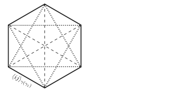
Figure 2: Convention of the quadratic correlations in Table 1. $\langle.\rangle$, $[.]$ and $(.)$ denote the first, second and third nearest-neighbor (NN) bonds, respectively. $\gamma=x,y,z$ label the type of a NN bond. $\gamma_{1},\gamma_{2}$ correspond to the two connecting NN bonds. $c=\gamma$ is determined by the parallel NN bond. $\alpha,\beta,\gamma$ ($a,b,c$) are mutually orthogonal. $C^{R}_{6}$ is a symmetry that rotates the six spins on a hexagon (anti-)clockwise. $C_{3}^{S}$ denote (anti-)cyclic permutations of the three spin components.

Furthermore, in addition to the constraints for ground states, in the $U(1)_{g}$ region in the phase diagram Figure 1 (c), we identify two field-induced quadratic correlations. The two correlations, denoted as $G^{h}_{1}$ and $G^{h}_{2}$ in Table 1, are invariant under global rotations about the direction of the $\vec{h}_{\rm 111}$ fields. From general symmetry principle, a continuous global symmetry will naturally support gapless modes. Hence, aside from being different local observables in the classical AFM Kitaev model, they may also shine light on the nature of the corresponding gapless quantum spin liquid Motome and Nasu (2020); Zhu et al. (2018); Hickey and Trebst (2019); Hickey et al. (2020); Zhu et al. (2020).

Note that the GSCs and other quadratic correlations learned by TK-SVM are not limited to classical spins. Their formalism holds for general spin-$S$ and can be directly measured in the quantum $K$-$\Gamma$ model. Comparing to other quantities (such as plaquette fluxes, Wilson/Polyakov loops, and spin structure factors), which may exhibit similar behaviors in different spin liquids, GSCs can be made unique to a ground-state manifold and hence may be more distinctive. Moreover, their violation provides a natural way to measure the breakdown of a spin liquid, which is what we use to estimate the extension of KSLs (see Appendix C).

V Cooperative and competitive constraint-induced ordering

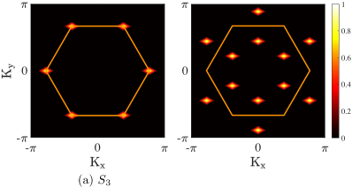
Figure 3: Static spin-structure factors (SSFs), $S(\vec{K})=\big{\langle}\frac{1}{N}\sum_{ij}\vec{S}_{i}\cdot\vec{S}_{j}\,e^{i\vec{K}\cdot(\vec{r}_{i}-\vec{r}_{j})}\big{\rangle}$, where $\vec{r}_{i}$ is the position of a spin at site $i$, and $\langle.\rangle$ denotes the ensemble average. The two $S_{3}$ orders develop magnetic Bragg peaks at the $\mathbf{K}$ points of the honeycomb Brillouin zone (orange hexagon). The two $S_{3}\times Z_{3}$ orders show Bragg peaks at $\frac{2}{3}\mathbf{M}$ points, owing to the larger magnetic cell. The length of nearest-neighbor bonds of the honeycomb lattice is set to unity.

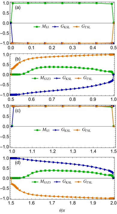
Figure 4: Measurements of the $S_{3}$ and modulated $S_{3}\times Z_{3}$ magnetizations (green), and characteristic Kitaev (blue) and $\Gamma$ (orange) correlations, with $K=\sin\theta$, $\Gamma=\cos\theta$, $h=0$, $T=0.001$. $M=\big{\langle}|\frac{1}{N_{\rm cell}}\sum_{\rm cell}\overrightarrow{M}|\big{\rangle}$ measures the magnitude of the respective magnetization, where $\overrightarrow{M}$ denotes the ordering moments in one magnetic cell, $\frac{1}{N_{\rm cell}}\sum_{\rm cell}(.)$ and $\langle.\rangle$ indicate the lattice and ensemble average, respectively. At the Kitaev ($\theta=\frac{\pi}{2},\frac{3\pi}{2}$) and $\Gamma$ ($\theta=0,\pi$) limits, either $G_{\rm KSL}=\pm 1$ or $G_{\rm\Gamma SL}=\pm 1$, satisfying the corresponding ground-state constraint. In the unfrustrated regions, $K\Gamma>0$, Kitaev and $\Gamma$ correlations behave in an equal footing as $G_{\rm KSL}=G_{\rm\Gamma SL}=\pm 1$, and cooperatively induce the AFM (a) or FM (c) $S_{3}$ order. In the frustrated regions, $K\Gamma<0$ [(b), (d)], $G_{\rm KSL}$ and $G_{\rm\Gamma SL}$ develop towards opposite directions. Though the system stays disordered near the Kitaev limits, from $|\Gamma/K|\sim 0.27$ up to the large $\Gamma$ limits, the $S_{3}\times Z_{3}$ orders are established owing to the competition between $G_{\rm KSL}$ and $G_{\rm\Gamma SL}$.

$\mathbf{S_{3}}$
$T_{1}$ $\left(\begin{array}[]{*{3}{@{}C{\mycolwd}@{}}}\displaystyle 1$\@add@centering&0$\@add@centering&0$\@add@centering\\ 0$\@add@centering&1$\@add@centering&0$\@add@centering\\ 0$\@add@centering&0$\@add@centering&1$\@add@centering\end{array}\right)$	$T_{2}=$ $\left(\begin{array}[]{*{3}{@{}C{\mycolwd}@{}}}\displaystyle 0$\@add@centering&1$\@add@centering&0$\@add@centering\\ 1$\@add@centering&0$\@add@centering&0$\@add@centering\\ 0$\@add@centering&0$\@add@centering&1$\@add@centering\end{array}\right)$	$T_{3}$ $\left(\begin{array}[]{*{3}{@{}C{\mycolwd}@{}}}\displaystyle 0$\@add@centering&0$\@add@centering&1$\@add@centering\\ 1$\@add@centering&0$\@add@centering&0$\@add@centering\\ 0$\@add@centering&1$\@add@centering&0$\@add@centering\end{array}\right)$	$T_{4}=$ $\left(\begin{array}[]{*{3}{@{}C{\mycolwd}@{}}}\displaystyle 0$\@add@centering&0$\@add@centering&1$\@add@centering\\ 0$\@add@centering&1$\@add@centering&0$\@add@centering\\ 1$\@add@centering&0$\@add@centering&0$\@add@centering\end{array}\right)$	$T_{5}$ $\left(\begin{array}[]{*{3}{@{}C{\mycolwd}@{}}}\displaystyle 0$\@add@centering&1$\@add@centering&0$\@add@centering\\ 0$\@add@centering&0$\@add@centering&1$\@add@centering\\ 1$\@add@centering&0$\@add@centering&0$\@add@centering\end{array}\right)$	$T_{6}=$ $\left(\begin{array}[]{*{3}{@{}C{\mycolwd}@{}}}\displaystyle 1$\@add@centering&0$\@add@centering&0$\@add@centering\\ 0$\@add@centering&0$\@add@centering&1$\@add@centering\\ 0$\@add@centering&1$\@add@centering&0$\@add@centering\end{array}\right)$
$\mathbf{Mod\ S_{3}\times Z_{3}}$
$T_{1}^{A}$ $\left(\begin{array}[]{*{3}{@{}C{\mycolwd}@{}}}\displaystyle 1$\@add@centering&0$\@add@centering&0$\@add@centering\\ 0$\@add@centering&1$\@add@centering&0$\@add@centering\\ 0$\@add@centering&0$\@add@centering&1$\@add@centering\end{array}\right)$	$T_{2}^{A}=$ $\left(\begin{array}[]{*{3}{@{}C{\mycolwd}@{}}}\displaystyle 0$\@add@centering&1$\@add@centering&0$\@add@centering\\ 1$\@add@centering&0$\@add@centering&0$\@add@centering\\ 0$\@add@centering&0$\@add@centering&-a$\@add@centering\end{array}\right)$	$T_{3}^{A}$ $\left(\begin{array}[]{*{3}{@{}C{\mycolwd}@{}}}\displaystyle 0$\@add@centering&0$\@add@centering&1$\@add@centering\\ -1/2$\@add@centering&0$\@add@centering&0$\@add@centering\\ 0$\@add@centering&-1/2$\@add@centering&0$\@add@centering\end{array}\right)$	$T_{4}^{A}=$ $\left(\begin{array}[]{*{3}{@{}C{\mycolwd}@{}}}\displaystyle 0$\@add@centering&0$\@add@centering&-a$\@add@centering\\ 0$\@add@centering&a-1$\@add@centering&0$\@add@centering\\ -a$\@add@centering&0$\@add@centering&0$\@add@centering\end{array}\right)$	$T_{5}^{A}$ $\left(\begin{array}[]{*{3}{@{}C{\mycolwd}@{}}}\displaystyle 0$\@add@centering&-1/2$\@add@centering&0$\@add@centering\\ 0$\@add@centering&0$\@add@centering&-1/2$\@add@centering\\ 1$\@add@centering&0$\@add@centering&0$\@add@centering\end{array}\right)$	$T_{6}^{A}=$ $\left(\begin{array}[]{*{3}{@{}C{\mycolwd}@{}}}\displaystyle 1$\@add@centering&0$\@add@centering&0$\@add@centering\\ 0$\@add@centering&0$\@add@centering&a-1$\@add@centering\\ 0$\@add@centering&a-1$\@add@centering&0$\@add@centering\end{array}\right)$
$T_{1}^{B}$ $\left(\begin{array}[]{*{3}{@{}C{\mycolwd}@{}}}\displaystyle-1/2$\@add@centering&0$\@add@centering&0$\@add@centering\\ 0$\@add@centering&-1/2$\@add@centering&0$\@add@centering\\ 0$\@add@centering&0$\@add@centering&-1/2$\@add@centering\end{array}\right)$	$T_{2}^{B}=$ $\left(\begin{array}[]{*{3}{@{}C{\mycolwd}@{}}}\displaystyle 0$\@add@centering&a-1$\@add@centering&0$\@add@centering\\ a-1$\@add@centering&0$\@add@centering&0$\@add@centering\\ 0$\@add@centering&0$\@add@centering&1$\@add@centering\end{array}\right)$	$T_{3}^{B}$ $\left(\begin{array}[]{*{3}{@{}C{\mycolwd}@{}}}\displaystyle 0$\@add@centering&0$\@add@centering&-1/2$\@add@centering\\ -1/2$\@add@centering&0$\@add@centering&0$\@add@centering\\ 0$\@add@centering&1$\@add@centering&0$\@add@centering\end{array}\right)$	$T_{4}^{B}=$ $\left(\begin{array}[]{*{3}{@{}C{\mycolwd}@{}}}\displaystyle 0$\@add@centering&0$\@add@centering&1$\@add@centering\\ 0$\@add@centering&-a$\@add@centering&0$\@add@centering\\ 1$\@add@centering&0$\@add@centering&0$\@add@centering\end{array}\right)$	$T_{5}^{B}$ $\left(\begin{array}[]{*{3}{@{}C{\mycolwd}@{}}}\displaystyle 0$\@add@centering&1$\@add@centering&0$\@add@centering\\ 0$\@add@centering&0$\@add@centering&-1/2$\@add@centering\\ -1/2$\@add@centering&0$\@add@centering&0$\@add@centering\end{array}\right)$	$T_{6}^{B}=$ $\left(\begin{array}[]{*{3}{@{}C{\mycolwd}@{}}}\displaystyle a-1$\@add@centering&0$\@add@centering&0$\@add@centering\\ 0$\@add@centering&0$\@add@centering&-a$\@add@centering\\ 0$\@add@centering&-a$\@add@centering&0$\@add@centering\end{array}\right)$
$T_{1}^{C}$ $\left(\begin{array}[]{*{3}{@{}C{\mycolwd}@{}}}\displaystyle-1/2$\@add@centering&0$\@add@centering&0$\@add@centering\\ 0$\@add@centering&-1/2$\@add@centering&0$\@add@centering\\ 0$\@add@centering&0$\@add@centering&-1/2$\@add@centering\end{array}\right)$	$T_{2}^{C}=$ $\left(\begin{array}[]{*{3}{@{}C{\mycolwd}@{}}}\displaystyle 0$\@add@centering&-a$\@add@centering&0$\@add@centering\\ -a$\@add@centering&0$\@add@centering&0$\@add@centering\\ 0$\@add@centering&0$\@add@centering&a-1$\@add@centering\end{array}\right)$	$T_{3}^{C}$ $\left(\begin{array}[]{*{3}{@{}C{\mycolwd}@{}}}\displaystyle 0$\@add@centering&0$\@add@centering&-1/2$\@add@centering\\ 1$\@add@centering&0$\@add@centering&0$\@add@centering\\ 0$\@add@centering&-1/2$\@add@centering&0$\@add@centering\end{array}\right)$	$T_{4}^{C}=$ $\left(\begin{array}[]{*{3}{@{}C{\mycolwd}@{}}}\displaystyle 0$\@add@centering&0$\@add@centering&a-1$\@add@centering\\ 0$\@add@centering&1$\@add@centering&0$\@add@centering\\ a-1$\@add@centering&0$\@add@centering&0$\@add@centering\end{array}\right)$	$T_{5}^{C}$ $\left(\begin{array}[]{*{3}{@{}C{\mycolwd}@{}}}\displaystyle 0$\@add@centering&-1/2$\@add@centering&0$\@add@centering\\ 0$\@add@centering&0$\@add@centering&1$\@add@centering\\ -1/2$\@add@centering&0$\@add@centering&0$\@add@centering\end{array}\right)$	$T_{6}^{C}=$ $\left(\begin{array}[]{*{3}{@{}C{\mycolwd}@{}}}\displaystyle-a$\@add@centering&0$\@add@centering&0$\@add@centering\\ 0$\@add@centering&0$\@add@centering&1$\@add@centering\\ 0$\@add@centering&1$\@add@centering&0$\@add@centering\end{array}\right)$

Table 2: Ordering matrices in the $S_{3}$ and modulated $S_{3}\times Z_{3}$ magnetizations. “$+$” (“$-$”) corresponds to the FM (AFM) $S_{3}$ order and the modulated $(S_{3}\times Z_{3})_{1(2)}$ order. $a\in[0,1]$ is $|\Gamma/K|$ dependent. The $S_{3}$ matrices form the symmetric group $S_{3}$. The $S_{3}\times Z_{3}$ matrices consist of three distinct $S_{3}$ sectors, featuring a spin-lattice entangled modulation $T^{A}_{k}+T^{B}_{k}+T^{C}_{k}=0$. A global sign difference is in $T_{k}$ with $k=2,4,6$, reflecting the sublattice symmetry of the Hamiltonian Eq. (1) in zero field.

A standard protocol to devise spin liquids is to introduce competing orders. In contrast to this familiar scenario, the emergence of the $S_{3}$ and the modulated $S_{3}\times Z_{3}$ orders are caused here by cooperation and competition between two spin liquids.

Unfrustrated $S_{3}$ orders. We first discuss the two $S_{3}$ phases in the unfrustrated regions $K\Gamma>0$. The discussion will also facilitate the understanding of the more exotic $S_{3}\times Z_{3}$ phases.

From the learned $C_{\mu\nu}$ matrices (see Appendix A), we identify that both $S_{3}$ orders have six magnetic sublattices with an order parameter

$$\overrightarrow{M}_{S_{3}}=\frac{1}{6}\sum_{k=1}^{6}T_{k}\vec{S}_{k},$$ (7)

where $T_{k}$ are ordering matrices, given in Table V, and the FM and AFM $S_{3}$ order differ by a global sign in $T_{2}$, $T_{4}$, and $T_{6}$. The six ordering matrices form the symmetric group $S_{3}$. Its cyclic subgroup, $C_{3}:=\{T_{1},T_{3},T_{5}\}$, are three-fold rotations about the $[111]$ direction in spin space, while $T_{2},T_{4}$ and $T_{6}$ correspond to reflection planes $(110),(011),(101)$, respectively. These matrices also reproduce the dual transformations that uncover the hidden $O(3)$ points residing at $K=\Gamma$ in the unfrustrated regions of the $K$-$\Gamma$ model Chaloupka and Khaliullin (2015).

The two $S_{3}$ orders feature the same static spin-structure factor (SSF). Both develop magnetic Bragg peaks at the K points of the honeycomb Brillouin zone (Figure 3), as the well-known $\sqrt{3}\times\sqrt{3}$ order. This highlights the importance of knowing explicit order parameters, as different phases may display identical features in momentum space.

Furthermore, we identify the other two GSCs,

$$G_{S_{3}}=\frac{1}{15}\langle\pm G_{1}\pm G_{2}+G_{3}+G_{4}\pm G_{5}\pm G_{6}\rangle_{\varhexagon}=1,$$ (8)

which equally comprise $G_{\rm KSL}$ and $G_{\rm\Gamma SL}$ in Eqs. (3)-(IV), with additional $G_{4}$ and $G_{6}$ terms owing to the normalization $|\vec{S}|=1$.

As we measure in Figure 4 (a), (c), in the spin-liquid limits $\theta\in\{0,\frac{\pi}{2},\pi,\frac{3\pi}{2}\}$, Kitaev and $\Gamma$ GSCs satisfy, as $G_{\rm KSL}=\pm 1$ or $G_{\rm\Gamma SL}=\pm 1$ with other correlations vanishing. However, when both $K$ and $\Gamma$ interactions are present and of the same sign, the two characteristic correlations $G_{\rm KSL}$ and $G_{\rm\Gamma SL}$ will lock together. This eliminates the local symmetries of Kitaev and $\Gamma$ spin liquids and gives way to the $S_{3}$ orders.

It is worth noting that the two $S_{3}$ phases also represent rare instances where magnetic states possess non-trivial GSCs, which normally exist in cases of classical spin liquids and multipolar orders Greitemann et al. (2019b).

Mod $S_{3}\times Z_{3}$ phases. The modulated $S_{3}\times Z_{3}$ orders can be measured by the order parameter

$$\overrightarrow{M}_{S_{3}\times Z_{3}}=\frac{1}{18}\sum_{\alpha}^{\scalebox{0.5}{A,B,C}}\sum_{k=1}^{6}T_{k}^{\alpha}\vec{S}_{k}^{\alpha},$$ (9)

where $T_{k}^{\alpha}$ are eighteen ordering matrices given in Table V, and $\alpha=A,B,C$ distinguish three different $S_{3}$ sectors as illustrated in Figure 1 (b). The $(S_{3}\times Z_{3})_{1}$ and $(S_{3}\times Z_{3})_{2}$ order differ by a global sign for all even $k$’s.

These orders exhibit a delicate spin-lattice entangled modulation,

$$T^{A}_{k}+T^{B}_{k}+T^{C}_{k}=0.$$ (10)

In concrete terms, $T^{\alpha}_{3,5}$ remain three-fold rotations along the $[111]$ direction, but there is an additional $\cos(2\pi/3)$ factor entering some, but not all, spin components. The location of this factor, as shown in Table V, alternates among the three $S_{3}$ sectors, to achieve the cancellation in Eq. (10). Furthermore, mirror reflections, $T^{\alpha}_{k}$ with even $k$’s are decorated by a factor $a\in[0,1]$, in such a way that a cancellation with the mirror of the same type occurs, as $(a-1)+(-a)+(1)=0$. The value of $a$, which TK-SVM also identifies, strongly depends on the relative strength $|\Gamma/K|$, while the reflection planes remain locked on $(110),(011),(101)$.

This modulation is very different from those in multiple-$\mathbf{q}$ orders and spin-density-wave (SDW) orders where phase factors universally act on all spin components. Moreover, since this modulation does not preserve spin length, the $S_{3}\times Z_{3}$ magnetization will not saturate to unity, but to a reduced value $M\lesssim\frac{2}{3}$, reflecting an intrinsic frustration.

The SSF of the two $S_{3}\times Z_{3}$ phases is shown in Figure 3 (b). The large magnetic cell leads to a reduced Brillouin zone. The SSF pattern nevertheless only partially reveals properties of the ordering and does not show information of the spin-lattice entangled modulation in Eq. (10), again underlining the significance of analytical order parameters.

To better understand the nature of the modulated $S_{3}\times Z_{3}$ orders, we show their magnetization along with the $G_{\rm KSL}$ and $G_{\rm\Gamma SL}$ correlations in Figure 4 (b) and (d). To exclude the $|K/\Gamma|$-dependence in the order parameter, we defined an alternative magnetization by including only odd $k$’s in Eq. (9), $\overrightarrow{M}^{\prime}_{S_{3}\times Z_{3}}=\frac{1}{9}\sum_{\alpha}^{\scalebox{0.5}{A,B,C}}\sum_{k}^{\scalebox{0.6}{1,3,5}}T_{k}^{\alpha}\vec{S}_{k}^{\alpha}$. Clearly, in the frustrated regions, the characteristic Kitaev and $\Gamma$ correlations develop toward opposite directions. Near the Kitaev limits, $\theta=\frac{\pi}{2},\frac{3\pi}{2}$, $G_{\rm KSL}$ dominates; the system stays disordered, either in an extended KSL phase or a CP region. When $G_{\rm\Gamma SL}$ is sufficiently strong to compete with $G_{\rm KSL}$, at $|\Gamma/K|\sim 0.27$, an $S_{3}\times Z_{3}$ order emerges from the two conflicting quadratic correlations, and expands till the large $\Gamma$ limits owing to the small exGSD of a $\Gamma$SL.

Because of the relevance to the spin-liquid candidate $\alpha$-$\mathrm{RuCl}_{3}$, (a part of) the parameter regime with FM $K$ and intermediate AFM $\Gamma$ has attracted much attention, as the $\Gamma$ term in this material is found to be comparable to the Kitaev interaction Ran et al. (2017); Kim and Kee (2016); Yadav et al. (2016); Winter et al. (2016). On the one hand, exact diagonalization (ED) of small systems Gordon et al. (2019), infinite density matrix renormalization group [(i)DMRG] simulations on narrow cylinders Gordon et al. (2019); Jiang et al. (2019); Gohlke et al. (2020), classical Luttinger-Tisza Rau et al. (2014), and cluster mean-field Rusnačko et al. (2019) analyses observed there a disordered phase or incommensurate order. On the other hand, classical simulated-annealing calculations for small system sizes Chern et al. (2020) and simple-update infinite projected-entangled-pair state (iPEPS) simulations Lee et al. (2020) reported magnetic states with enlarged unit cells but of unknown nature. Our results are compatible with the latter observations. The magnetic Bragg peaks (located at the $\frac{2}{3}{\bf M}$ points) of the $(S_{3}\times Z_{3})_{2}$ phase are consistent with the SSFs reported in Ref. Chern et al. (2020). However, our machine identifies the order parameter and the correlations underlying the phase.

The fate of the modulated $S_{3}\times Z_{3}$ order in quantum $K$-$\Gamma$ models, for the case of spin-$1/2$ as well as higher $S$ values, is open and left for future studies. It is however not uncommon that, when a system establishes a robust magnetic order in the classical large-$S$ limit, this order can persist in the quantum cases with a reduced ordering moment due to quantum fluctuations. Such examples are known for various spin-liquid candidates, see for instance Refs. Zheng et al. (2006); White and Chernyshev (2007); Li et al. (2018).

The firmness of the $S_{3}\times Z_{3}$ orders can be demonstrated in several ways. In Figure 4 (b) and (d), we confirm their stability by varying $\theta=\arctan(K/\Gamma)$ over the entire frustrated region. Moreover, the global phase diagram Figure 1 (c) shows that they are robust against finite fields. This is further verified in Appendix D where we show a direct Monte Carlo measurement of the $(S_{3}\times Z_{3})_{2}$ order and its suppression in intermediate fields. In addition, the stability of this order against thermal fluctuations, inevitable for real systems, is also established in Appendix D. Interestingly, the melting involves two stages and gives rise to an intermediate paramagnetic regime found for temperatures significantly below the Neel temperature.

From the machine learning point of view, the two modulated $S_{3}\times Z_{3}$ orders provide a hallmark of a machine-learning algorithm identifying different, complicated phases. Furthermore, the identification of the spin-liquid constraints also gives insight into their origin, by which the emergence of magnetic orders in the $K$-$\Gamma$ model can be consistently explained.

VI Conclusions

Machine learning techniques are emerging as promising tools in various disciplines of physics Carleo et al. (2019). However, results going beyond the state of the art are required before they will disrupt current procedures. By subjecting the honeycomb $K$-$\Gamma$-$h$ model to the analysis of our unsupervised and interpretable TK-SVM method, we have shown that machine learning can indeed handle highly complicated problems in frustrated magnets and reveal unknown physics.

We found that the classical phase diagram of the $K$-$\Gamma$ model in an $[111]$ field is exceptionally rich (see Figure 1), hosting several unconventional symmetry-breaking phases and a plethora of disordered states at very low temperature. The phase diagram clearly shows the finite extent of the KSLs, an intermediate disordered phase at the AFM Kitaev limit, and a field-induced suppression of magnetic orders, which were previously only reported for quantum systems. These common features strongly suggest that certain aspects of the Kitaev materials can already be understood from a semi-quantitative classical picture and also call for a systematic investigation of larger spin models in order to find potential higher-$S$ spin liquids.

Two phases, the modulated $S_{3}\times Z_{3}$ magnets, with a previously unknown type of modulation were identified. On the one hand, these states represent a concrete instance of machine learning successfully discovering novel phases. Their structure is sufficiently complicated, but it is picked up without difficulty by TK-SVM. On the other hand, they also imply that the competition between Kitaev and non-Kitaev exchanges can significantly enrich the physics and lead to more unconventional phases than expected.

We discovered the GSCs of the classical $\Gamma$SLs and reproduced the ones of the KSLs. Not only did these constraints enhance our understanding of the $\Gamma$SLs, they also put the emergence of the complicated orders in the $K$-$\Gamma$ model in a unifying picture. The two unfrustrated $S_{3}$ magnets emerge when the characteristic Kitaev and $\Gamma$ correlations cooperatively eliminate the macroscopic degeneracy of each other. By contrast, the two modulated $S_{3}\times Z_{3}$ magnets can be understood as the consequence of the competition between the KSL and $\Gamma$SL. This mechanism may be viewed as an alternative protocol for devising exotic phases.

Our work may stimulate future applications of machine learning in Kitaev materials and beyond. The study of Kitaev materials is motivated by realizing the Kitaev model Jackeli and Khaliullin (2009); Chaloupka et al. (2010). In real systems, non-Kitaev interactions are ubiquitously present and cannot be treated as perturbations. In the case of $\alpha$-$\mathrm{RuCl}_{3}$, aside from the dominating Kitaev and $\Gamma$ exchanges, the Heisenberg $J_{1}$, $J_{3}$, and, possibly, the off-diagonal $\Gamma^{\prime}$ term also play a role Laurell and Okamoto (2020); Maksimov and Chernyshev (2020). Temperature and external fields add further dimensions to the physical parameter space Kasahara et al. (2018); Banerjee et al. (2017); Bachus et al. (2020). Similar complications are also encountered in other candidate compounds such as ${\rm A}_{2}{\rm IrO}_{3}$ ($\rm{A}={\rm Na,K}$) Yadav et al. (2018, 2019) and the three-dimensional hyper- and stripy-honeycomb materials $\beta$-, $\gamma$-${\rm Li}_{2}{\rm IrO}_{3}$ Modic et al. (2014); Takayama et al. (2015); Biffin et al. (2014). While these additional terms besides the Kitaev exchange can enrich the underlying physics, they also dramatically complicate the analysis. Machine learning is designed to discover complex structures in high-dimensional data. In the framework of TK-SVM, partitioning a phase diagram can be formulated as a two-dimensional Laplacian matrix Fiedler (1973, 1975), independent of the number of physical parameters. This ability permits an efficient scanning over complex, multi-dimensional phase diagrams. The nature of each phase will also be uncovered in virtue of the machine’s interpretability. TK-SVM may hence speed up our understanding of competing interactions in a multi-dimensional parameter space, which can in turn facilitate the experimental search and theoretical development for exotic phases.

Open source and data availability

The TK-SVM library has been made openly available with documentation and examples Greitemann et al. . The data used in this work are available upon request.

Appendix A Setting up of TK-SVM

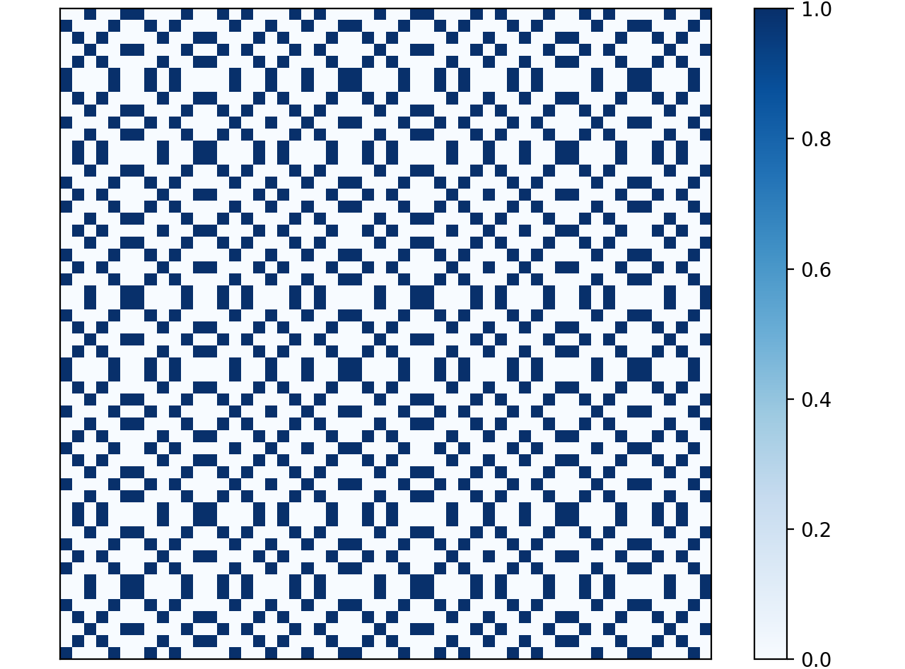
(a) FM $S_{3}$

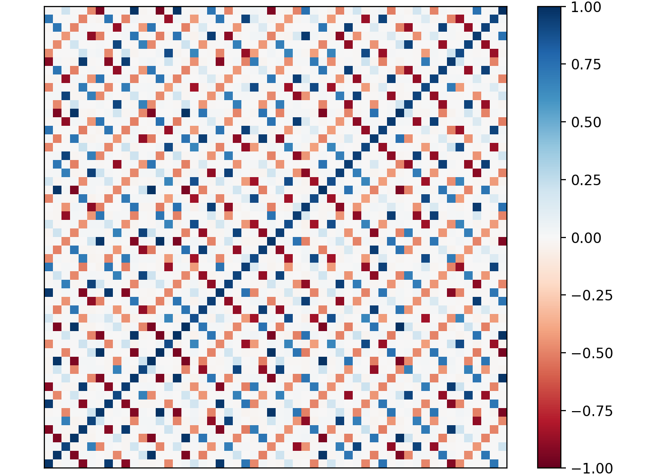
(b) mod $(S_{3}\times Z_{3})_{2}$

Figure 5: Visualization of the $C_{\mu\nu}$ matrix of the FM $S_{3}$ and the mod $(S_{3}\times Z_{3})_{2}$ phase. Each pixel corresponds to an entry of $C_{\mu\nu}$. Non-vanishing entries identify the relevant components of $\phi_{\mu}$ entering the order parameter. Here results of a $18$-spin cluster are shown for demonstration, while much larger clusters are used for the phase diagram Figure 1. The $S_{3}$ order is represented multiple times as its magnetic cell has six sublattices.

The TK-SVM method has been introduced in our previous work Greitemann et al. (2019a); Liu et al. (2019); Greitemann et al. (2019b). Here we review its essential ingredients for completeness.

For a sample $\mathbf{x}=\{S_{i}^{a}|i=1,2,...,N;a=x,y,z\}$, the feature vector $\bm{\phi}=\{\phi_{\mu}\}$ maps $\mathbf{x}$ to degree-$n$ monomials

$$\phi_{\mu}=\langle S_{\alpha_{1}}^{a_{1}}S_{\alpha_{2}}^{a_{2}}\dots S_{\alpha_{n}}^{a_{n}}\rangle_{\rm cl},$$ (11)

where $\langle\cdots\rangle_{\rm cl}$ represents a lattice average up to a cluster of $r$ spins; $\alpha_{1},\dots,\alpha_{n}$ label spins in the cluster; $\mu=\{\alpha_{1},a_{1};\dots,\alpha_{n},a_{n}\}$ are collective indices.

TK-SVM constructs from $\phi_{\mu}$ a tensorial feature space ($\bm{\phi}$-space) to host potential orders Greitemann et al. (2019a); Liu et al. (2019). The capacity of the $\bm{\phi}$-space depends on the degree ($n$) of monomials and the size ($r$) of the cluster. As the minimal $n$ and $r$ are unknown parameters, in practice, we choose large clusters according to the Bravais lattice and $n\in~{}[1,6]$, where $n=1$ detects magnetic orders and $n>1$ probes multipolar orders and emergent local constraints. In learning the phase diagram Figure 1, we constructed $\bm{\phi}$-spaces using clusters up to $288$ spins ($12\times 12$ honeycomb unit-cells) at rank-$1$ and clusters up to $18$ spins at rank-$2$, much beyond the needed capacity. We also confirmed the results are consistent when varying the size and shape of clusters and found ranks $n\geq 3$ to be irrelevant.

The coefficient matrix $\mathbbm{C}=\{C_{\mu\nu}\}$ measures correlations of $\phi_{\mu}$, defined as

$$C_{\mu\nu}=\sum_{k}\lambda_{k}\phi_{\mu}(\mathbf{x}^{(k)})\phi_{\nu}(\mathbf{x}^{(k)}),$$ (12)

where the Lagrange multiplier $\lambda_{k}$ denotes the weight of the $k$-th sample and is solved in the underlying SVM optimization problem Greitemann et al. (2019a); Liu et al. (2019). Its non-vanishing entries identify the relevant basis tensors of the $\bm{\phi}$-space, and their interpretation leads to order parameters.

In Figure 5, we show the $C_{\mu\nu}$ matrix of the FM $S_{3}$ and the mod $(S_{3}\times Z_{3})_{2}$ phase for example. The corresponding order parameters are given in Eqs. (7) and (9) and are measured in Figure 4 in the main text.

Appendix B Details of Graph Partitioning

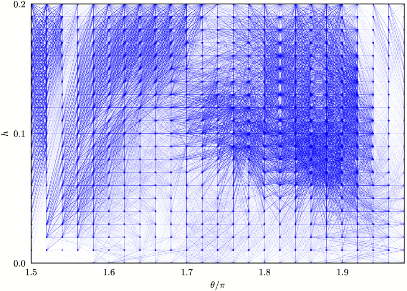
Figure 6: The $\theta\in[\frac{3\pi}{2},2\pi)$ sector of the graph is shown for visualization. Each vertex labels a $(\theta,h)$ point, following a uniform distribution $\Delta\theta=0.02\pi$, $\Delta h=0.01$. The edges connecting two vertices are determined by $\rho$ in the corresponding decision function and the weight function Eq. (14). Edge weights are weakened to reduce visual density. The entire graph contains $M=1,\!250$ vertices with $\theta\in[0,2\pi)$ and $M(M-1)/2=780,\!625$ edges, whose partition gives the phase diagram Figure 1 (c).

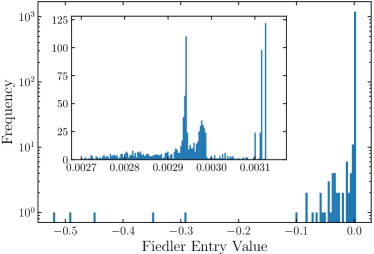
Figure 7: Histogram of Fiedler vector entries. Each entry corresponds to a vertex of the graph, namely, a $(\theta,h)$ point. Their values are color-coded by the phase diagram Figure 1 (c). A logarithmic scale is used in the main panel as the histogram is spanning several orders. The inner panel uses a linear scale and shows a zoom-in view of the bulk of the distribution. From left to right, the five profound peaks in the inner panel correspond to the two $S_{3}\times Z_{3}$ phases, the FM $S_{3}$, the AFM $S_{3}$ phase and the full polarized phase, respectively. Flat regions correspond to correlated paramagnets and indicate wide crossovers to neighboring phases.

Not all $C_{\mu\nu}$ matrices need to be interpreted. In the graph partitioning, where the goal is to learn the topology of the phase diagram, it suffices to analyze the bias parameter $\rho$. When ${\rm A,B}$ are two phase points where spin configurations are generated, the bias parameter $\rho_{\rm AB}$ in the corresponding binary classification problem behaves as

$$|\rho_{\rm AB}|\begin{cases}\gg 1&\textup{${\rm A,B}$ in the same phase},\\ \lesssim 1&\textup{${\rm A,B}$ in different phases}.\end{cases}$$ (13)

Thus, as demonstrated in our previous work, $\rho$ can detect phase transitions and crossovers Liu et al. (2019); Greitemann et al. (2019b). (Though the sign of $\rho_{\rm AB}$ also has physical meaning and can reveal which phase is in the (dis-)ordered side, the absolute value is sufficient for the graph partitioning; see Ref. Greitemann et al., 2019b for details.)

The graph partitioning in TK-SVM is a systematic application of the $\rho$ criteria Eq. (13). The graph is built from $M=1,\!250$ vertices, each corresponding to a point $(\theta,h)$, and $M(M-1)/2$ connecting edges; as exemplified in Figure 6. The weight of an edge is defined by $\rho$ in the SVM classification between the two endpoints, with a Lorentzian weighting function

$$w(\rho) =1-\frac{\rho_{c}^{2}}{(|\rho|-1)^{2}+\rho_{c}^{2}}\in[0,1].$$ (14)

Here $\rho_{c}$ sets a characteristic scale for “$\gg 1$” in Eq. (13), as a larger $\rho_{c}$ tends to suppress weight of the edges. The choice of $\rho_{c}$ is not critical since points in the same phase are always more connected than those from different phases. In computing the phase diagram Figure 1, $\rho_{c}=1000$ is applied, but we also verified that the results are robust when $\rho_{c}$ is changed over an interval ranging from a small $\rho_{c}=10$ to a large $\rho_{c}=10^{4}$, where all edge weights are almost eliminated.

A graph with $10^{6}$ edges is considered a small problem in graph theory and may be partitioned with different methods. We have applied Fiedler’s theory of spectral clustering Fiedler (1973, 1975). The result is a so-called Fiedler vector of the dimensionality $M$, corresponding to the $M$ vertices. Strongly connected vertices, namely those in the same phase, share equal or very close Fiedler-entry values, while those in different phases have substantially different Fiedler entries. In this sense, the Fiedler vector can act as a phase diagram.

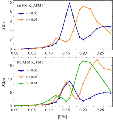
Figure 8: Susceptibility for the characteristic Kitaev correlation $G_{\rm KSL}$ as function of $|\Gamma/K|$, in the vicinity of the FM (a) and AFM (b) Kitaev limit with $K\Gamma\leq 0$. The first peak of $\chi_{\rm G_{KSL}}$ in a fixed $h$ identifies the crossover from a classical KSL to a non-Kitaev correlated paramagnet. At $h=0$, the KSLs survive until $|\Gamma/K|\sim 0.16$. When magnetic fields are applied, the peak moves consistently towards a smaller value of $|\Gamma/K|$ with its width broadening. The wide bumps at lager $|\Gamma/K|$ signal the second crossover to a modulated $S_{3}\times Z_{3}$ phase, for which the optimal quantity is the $S_{3}\times Z_{3}$ magnetization.

Note that, the two-dimensional representation of the graph shown in Figure 6 is only for visualization. Regardless of the dimension of a physical parameter space, a graph can always be formulated by a Laplacian matrix, and its partitioning gives a vectorial quantity, i.e., the Fiedler vector Fiedler (1973, 1975); Liu et al. (2019).

Figure 7 shows the histogram of the Fiedler entries for the phase diagram Figure 1 (c), which clearly exhibit a multinodal structure. Each peak corresponds to a distinct phase, and the wide bumps are indicative of crossover regions or phase boundaries.

Figure 9: Field dependence of the magnetization per spin parallel ($m_{\parallel}$) and perpendicular ($m_{\perp}$) to the $[111]$ field, and the normalized $U(1)_{g}$-symmetric correlations, $G^{h}_{1}$ and $G^{h}_{2}$, at the AFM Kitaev limit $(K,\Gamma)=(1,0)$. The spins are mostly paramagnetic under weak and intermediate fields. Bumps in $dG^{h}/dh$ may imply prominent changes in the system.

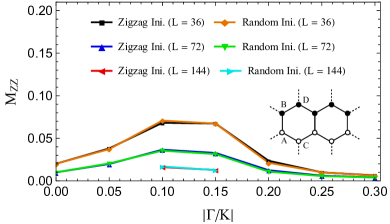
Figure 10: Monte Carlo measurement of the zigzag order in the region of FM $K$ and small AFM $\Gamma$ at $h=0$, where the magnetization $M_{\rm ZZ}=\big{\langle}\big{|}\frac{1}{N_{\rm cell}}\sum_{\rm cell}\big{(}\vec{S}_{A}-\vec{S}_{B}+\vec{S}_{C}-\vec{S}_{D}\big{)}\big{|}\big{\rangle}$, and $A,B,C,D$ label the four sub-lattices. Simulations initiated with perfect zigzag states are compared with random initializations. The zigzag order appears to be unstable in all cases. The small residual moments are a finite-size effect and decrease significantly with increasing system sizes.

Appendix C Extension of Classical KSLs

Since a GSC, $G$, characterizes a classical spin liquid, we can accordingly define a susceptibility to measure how sharp it is defined,

$$\chi_{\rm G}=\frac{V}{T}\left(\langle G^{2}\rangle-\langle G\rangle^{2}\right),$$ (15)

where $\langle\dots\rangle$ is the ensemble average, and $V$ denotes the volume of the system. Such a susceptibility was first introduced in Ref. Greitemann et al. (2019b), and we showed with various examples its high sensitivity to the breakdown of an associated classical spin liquid.

To estimate the extension of classical KSLs, we define the susceptibility $\chi_{\rm G_{KSL}}$. It is shown in Figure 8 as a function of the competing $\Gamma$ interaction. At a fixed $h$, $\chi_{\rm G_{KSL}}$ develops two peaks/bumps, reflecting the violation of the GSC. The sharper peak at a smaller $|\Gamma/K|$ is responsible for the crossover between a KSL and a non-Kitaev correlated paramagnet. The broad bump at a larger $|\Gamma/K|$ signals the second crossover to a modulated $S_{3}\times Z_{3}$ phase. (The optimal measure to this second crossover is the $S_{3}\times Z_{3}$ order parameter instead of $\chi_{\rm G_{KSL}}$. However, the location of the bump qualitatively agrees with the results based on the $S_{3}\times Z_{3}$ magnetization, see Figure 4 for example.)

In order to examine the effects of magnetic fields on the AFM KSL, we measure the field-dependence of the two $U(1)_{g}$-symmetric correlations, $G^{h}_{1}$ and $G^{h}_{2}$, and the magnetization per spin parallel ($m_{\parallel}$) and perpendicular ($m_{\perp}$) to the $[111]$ field, as is shown in Figure 9. Under weak and intermediate fields, most of the spins respond paramagnetically, as $m_{\parallel}$ is small and $m_{\perp}$ vanishes. While $G^{h}_{1}$ and $G^{h}_{2}$ smoothly increase with the external field, the bumps in their derivative may imply prominent changes in the system, which are used to estimate the extent of the AFM KSL. The regime with intermediate field is marked as a $U(1)_{g}$ region in order to distinguish it from a polarized state. In the main text (see Sections III and IV), we discussed that this regime coincides with a gapless spin liquid proposed for quantum spin-$1/2$ and spin-$1$ AFM Kitaev models Motome and Nasu (2020); Zhu et al. (2018); Hickey and Trebst (2019); Hickey et al. (2020); Zhu et al. (2020). A similar segmentation in the finite-$h$ phase diagram is observed in the quantum case Zhu et al. (2018, 2020).

The behavior of $\chi_{\rm G_{KSL}}$, $G^{h}_{1}$, and $G^{h}_{2}$ are used to estimate the boundary (indicated by the dashed lines in Figure 1 (c)) between the KSLs and other correlated paramagnets, supplementing the graph partitioning. This is needed because, in the graph partitioning shown in Figure 1, we only employed a rank-$1$ TK-SVM which is designed for detecting the presence and absence of magnetic order. To classify different spin liquids, we use rank-$2$ TK-SVM to identify their GSCs. In principle, we could also have performed a separate graph partitioning with rank-$2$ TK-SVM. But, given the rank-$1$ results, most of the phase diagram has already been fully classified this way and there are only few locations left worth examining at higher rank.

In Figure 10 we evaluate the zigzag magnetization in the extended KSL and CP region with FM $K$ and AFM $\Gamma$. The zigzag order has been considered as a $\Gamma$-induced competing order to a KSL. However, it can be shown that it is unstable at low temperature and experiences strong finite-size effects. This is also consistent with the picture that, in order to stabilize the zigzag-like order found in $\alpha$-$\mathrm{RuCl}_{3}$ Banerjee et al. (2017); Ran et al. (2017), other terms, such as the first and third nearest-neighbor Heisenberg $J_{1}$, $J_{3}$ interactions Gohlke et al. (2018); Gass et al. (2020); Jiang et al. (2019) or the off-diagonal $\Gamma^{\prime}$ term Gordon et al. (2019); Lee et al. (2020); Gohlke et al. (2020); Chern et al. (2020), are needed.

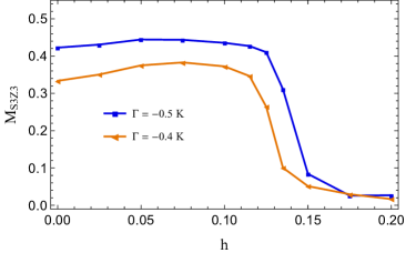
Figure 11: Monte Carlo measurement of the $(S_{3}\times Z_{3})_{2}$ magnetization as a function of the $[111]$ field, in the region of FM $K$ and intermediate AFM $\Gamma$. The $(S_{3}\times Z_{3})_{2}$ magnetization extends over a finite region of external field and is subsequently suppressed to a small but finite value, see Figure 1(c).

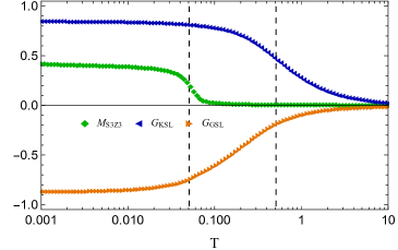
Figure 12: Temperature dependence of the $(S_{3}\times Z_{3})_{2}$ order and the corresponding Kitaev and $\Gamma$ correlations for $h=0$, $\Gamma=-0.5$, and $K>0$. The system exhibits a two-step melting, dividing the temperature range into three regimes. In the low-temperature regime, the $(S_{3}\times Z_{3})_{2}$ order is established along with strong $G_{\rm KSL}$ and $G_{\rm\Gamma SL}$. The intermediate regime is a correlated paramagnet, where the competing Kitaev and $\Gamma$ correlations are already noticeable but not strong enough to stabilize magnetic order. A trivial paramagnet is found for high temperatures. The dashed lines mark the location of crossovers.

Appendix D Field and temperature dependence of the modulated $(S_{3}\times Z_{3})_{2}$ order

The machine-learned global phase diagram Figure 1 (c) shows that the modulated $S_{3}\times Z_{3}$ orders extend over a finite region of a $[111]$ field. In particular, in the parameter regime relevant for $\alpha$-$\mathrm{RuCl}_{3}$, namely a FM $K$ and an intermediate AFM $\Gamma$, the $(S_{3}\times Z_{3})_{2}$ order experiences a field-induced suppression. This is further confirmed in Figure 11 by direct measurement of the $S_{3}\times Z_{3}$ magnetization. After suppressing the order, the system enters a partially-polarized frustrated regime, owing to the competition between the external field and the Kitaev and $\Gamma$ interactions. A similar classical regime was discussed in Ref. Gohlke et al. (2020) and was considered as the parent phase of two quantum nematic paramagnets in the spin-$1/2$ $K$-$\Gamma$ model Gohlke et al. (2020); Lee et al. (2020).

In Figure 12, we evaluate the temperature dependence of the $(S_{3}\times Z_{3})_{2}$ magnetization and the corresponding Kitaev and $\Gamma$ correlations. The system exhibits two crossovers when increasing temperature. Order is established in the low-temperature regime with strong $G_{\rm KSL}$ and $G_{\rm\Gamma SL}$. Its melting is followed by an intermediate regime where the Kitaev and $\Gamma$ correlations already develop but are not yet strong enough to stabilize magnetic order. This is consistent with the scenario discussed in Section V that the $S_{3}\times Z_{3}$ order can be understood from the competition between the two quadratic correlations. This intermediate regime also extends until nearly one order below the Neel temperature which is set by the interaction strength, and may hence be viewed as a finite-temperature correlated paramagnet.

While a two-step melting is often observed for spin liquids, including the quantum KSL Motome and Nasu (2020); Nasu et al. (2017) and the classical $\Gamma$SL Saha et al. (2019), as well as for spin nematics, such as the multipolar orders in the Kagome Zhitomirsky (2008) and pyrochlore Taillefumier et al. (2017) anti-ferromagnets, such a phenomenon is quite unusual for a magnetically ordered system. We leave for future studies to find out what type of excitations are responsible for the two crossovers, and whether such a two-step melting can also be present when other interactions that can exist in real materials are included.

The $(S_{3}\times Z_{3})_{1}$ phase has the same temperature dependence because of the sub-lattice symmetry of the $K$-$\Gamma$ model at zero field. However, the sign of $G_{\rm KSL}$ and $G_{\rm\Gamma SL}$ is swapped as in the case of Figure 4 (b) and (d).

References

- Kitaev (2006) Alexei Kitaev, “Anyons in an exactly solved model and beyond,” Ann. Phys. (N. Y.) 321, 2–111 (2006), january Special Issue.
- Jackeli and Khaliullin (2009) G. Jackeli and G. Khaliullin, “Mott Insulators in the Strong Spin-Orbit Coupling Limit: From Heisenberg to a Quantum Compass and Kitaev Models,” Phys. Rev. Lett. 102, 017205 (2009).
- Chaloupka et al. (2010) J. Chaloupka, George Jackeli, and Giniyat Khaliullin, “Kitaev-Heisenberg Model on a Honeycomb Lattice: Possible Exotic Phases in Iridium Oxides ,” Phys. Rev. Lett. 105, 027204 (2010).
- Takagi et al. (2019) Hidenori Takagi, Tomohiro Takayama, George Jackeli, Giniyat Khaliullin, and Stephen E. Nagler, “Concept and realization of Kitaev quantum spin liquids,” Nat. Rev. Phys. 1, 264–280 (2019).
- Winter et al. (2017a) Stephen M Winter, Alexander A Tsirlin, Maria Daghofer, Jeroen van den Brink, Yogesh Singh, Philipp Gegenwart, and Roser Valentí, “Models and materials for generalized Kitaev magnetism,” Journal of Physics: Condensed Matter 29, 493002 (2017a).
- Kasahara et al. (2018) Y. Kasahara, T. Ohnishi, Y. Mizukami, O. Tanaka, Sixiao Ma, K. Sugii, N. Kurita, H. Tanaka, J. Nasu, Y. Motome, T. Shibauchi, and Y. Matsuda, “Majorana quantization and half-integer thermal quantum hall effect in a Kitaev spin liquid,” Nature 559, 227–231 (2018).
- Yokoi et al. (2020) T Yokoi, S Ma, Y Kasahara, S Kasahara, T Shibauchi, N Kurita, H Tanaka, J Nasu, Y Motome, C Hickey, S. Trebst, and Y. Matsuda, “Half-integer quantized anomalous thermal Hall effect in the Kitaev material ,” arXiv preprint arXiv:2001.01899 (2020).
- Kitagawa et al. (2018) K. Kitagawa, T. Takayama, Y. Matsumoto, A. Kato, R. Takano, Y. Kishimoto, S. Bette, R. Dinnebier, G. Jackeli, and H. Takagi, “A spin–orbital-entangled quantum liquid on a honeycomb lattice,” Nature 554, 341–345 (2018).
- Takahashi et al. (2019) Sean K. Takahashi, Jiaming Wang, Alexandre Arsenault, Takashi Imai, Mykola Abramchuk, Fazel Tafti, and Philip M. Singer, “Spin Excitations of a Proximate Kitaev Quantum Spin Liquid Realized in ,” Phys. Rev. X 9, 031047 (2019).
- Song et al. (2016) Xue-Yang Song, Yi-Zhuang You, and Leon Balents, “Low-energy spin dynamics of the honeycomb spin liquid beyond the Kitaev limit,” Phys. Rev. Lett. 117, 037209 (2016).
- Kimchi and You (2011) Itamar Kimchi and Yi-Zhuang You, “Kitaev-Heisenberg-- model for the iridates IrO3,” Phys. Rev. B 84, 180407 (2011).
- Singh et al. (2012) Yogesh Singh, S. Manni, J. Reuther, T. Berlijn, R. Thomale, W. Ku, S. Trebst, and P. Gegenwart, “Relevance of the Heisenberg-Kitaev Model for the Honeycomb Lattice Iridates ,” Phys. Rev. Lett. 108, 127203 (2012).
- Price and Perkins (2012) Craig C. Price and Natalia B. Perkins, “Critical properties of the Kitaev-Heisenberg model,” Phys. Rev. Lett. 109, 187201 (2012).
- Li et al. (2015) Kai Li, Shun-Li Yu, and Jian-Xin Li, “Global phase diagram, possible chiral spin liquid, and topological superconductivity in the triangular Kitaev–Heisenberg model,” New Journal of Physics 17, 043032 (2015).
- Sears et al. (2015) J. A. Sears, M. Songvilay, K. W. Plumb, J. P. Clancy, Y. Qiu, Y. Zhao, D. Parshall, and Young-June Kim, “Magnetic order in : A honeycomb-lattice quantum magnet with strong spin-orbit coupling,” Phys. Rev. B 91, 144420 (2015).
- Janssen et al. (2016) Lukas Janssen, Eric C. Andrade, and Matthias Vojta, “Honeycomb-lattice Heisenberg-Kitaev model in a magnetic field: Spin canting, metamagnetism, and vortex crystals,” Phys. Rev. Lett. 117, 277202 (2016).
- Janssen et al. (2017) Lukas Janssen, Eric C. Andrade, and Matthias Vojta, “Magnetization processes of zigzag states on the honeycomb lattice: Identifying spin models for and ,” Phys. Rev. B 96, 064430 (2017).
- Jiang et al. (2019) Yi-Fan Jiang, Thomas P. Devereaux, and Hong-Chen Jiang, “Field-induced quantum spin liquid in the Kitaev-Heisenberg model and its relation to ,” Phys. Rev. B 100, 165123 (2019).
- Chern et al. (2020) Li Ern Chern, Ryui Kaneko, Hyun-Yong Lee, and Yong Baek Kim, “Magnetic field induced competing phases in spin-orbital entangled Kitaev magnets,” Phys. Rev. Research 2, 013014 (2020).
- Gordon et al. (2019) Jacob S. Gordon, Andrei Catuneanu, Erik S. Sørensen, and Hae-Young Kee, “Theory of the field-revealed Kitaev spin liquid,” Nature Communications 10, 2470 (2019).
- Wang et al. (2019) Jiucai Wang, B. Normand, and Zheng-Xin Liu, “One Proximate Kitaev Spin Liquid in the Model on the Honeycomb Lattice,” Phys. Rev. Lett. 123, 197201 (2019).
- Lee et al. (2020) Hyun-Yong Lee, Ryui Kaneko, Li Ern Chern, Tsuyoshi Okubo, Youhei Yamaji, Naoki Kawashima, and Yong Baek Kim, “Magnetic field induced quantum phases in a tensor network study of Kitaev magnets,” Nature Communications 11, 1639 (2020).
- Gohlke et al. (2018) Matthias Gohlke, Gideon Wachtel, Youhei Yamaji, Frank Pollmann, and Yong Baek Kim, “Quantum spin liquid signatures in Kitaev-like frustrated magnets,” Phys. Rev. B 97, 075126 (2018).
- Gohlke et al. (2020) Matthias Gohlke, Li Ern Chern, Hae-Young Kee, and Yong Baek Kim, “Emergence of a nematic paramagnet via quantum order-by-disorder and pseudo-goldstone modes in Kitaev magnets,” arXiv preprint arXiv:2003.11876 (2020).
- Osorio Iregui et al. (2014) Juan Osorio Iregui, Philippe Corboz, and Matthias Troyer, “Probing the stability of the spin-liquid phases in the Kitaev-Heisenberg model using tensor network algorithms,” Phys. Rev. B 90, 195102 (2014).
- Gohlke et al. (2017) Matthias Gohlke, Ruben Verresen, Roderich Moessner, and Frank Pollmann, “Dynamics of the Kitaev-Heisenberg model,” Phys. Rev. Lett. 119, 157203 (2017).
- Motome and Nasu (2020) Yukitoshi Motome and Joji Nasu, “Hunting majorana fermions in Kitaev magnets,” Journal of the Physical Society of Japan 89, 012002 (2020).
- Zhu et al. (2018) Zheng Zhu, Itamar Kimchi, D. N. Sheng, and Liang Fu, “Robust non-abelian spin liquid and a possible intermediate phase in the antiferromagnetic Kitaev model with magnetic field,” Phys. Rev. B 97, 241110 (2018).
- Hickey and Trebst (2019) Ciarán Hickey and Simon Trebst, “Emergence of a field-driven U(1) spin liquid in the Kitaev honeycomb model,” Nature Communications 10, 530 (2019).
- Hickey et al. (2020) Ciarán Hickey, Christoph Berke, Panagiotis Peter Stavropoulos, Hae-Young Kee, and Simon Trebst, “Field-driven gapless spin liquid in the spin-1 Kitaev honeycomb model,” Phys. Rev. Research 2, 023361 (2020).
- Zhu et al. (2020) Zheng Zhu, Zheng-Yu Weng, and D. N. Sheng, “Magnetic field induced spin liquids in Kitaev honeycomb model,” Phys. Rev. Research 2, 022047 (2020).
- Don (2020) “Spin-1 Kitaev-Heisenberg model on a honeycomb lattice, author = Dong, Xiao-Yu and Sheng, D. N.” Phys. Rev. B 102, 121102 (2020).
- Berke et al. (2020) Christoph Berke, Simon Trebst, and Ciarán Hickey, “Field stability of Majorana spin liquids in antiferromagnetic Kitaev models,” Phys. Rev. B 101, 214442 (2020).
- Khait et al. (2020) Ilia Khait, P Peter Stavropoulos, Hae-Young Kee, and Yong Baek Kim, “Characterizing spin-one Kitaev quantum spin liquids,” arXiv preprint arXiv:2001.06000 (2020).
- Rousochatzakis et al. (2015) Ioannis Rousochatzakis, Johannes Reuther, Ronny Thomale, Stephan Rachel, and N. B. Perkins, “Phase Diagram and Quantum Order by Disorder in the Kitaev Honeycomb Magnet,” Phys. Rev. X 5, 041035 (2015).
- Stavropoulos et al. (2019) P. Peter Stavropoulos, D. Pereira, and Hae-Young Kee, “Microscopic mechanism for a higher-spin Kitaev model,” Phys. Rev. Lett. 123, 037203 (2019).
- Xu et al. (2020) Changsong Xu, Junsheng Feng, Mitsuaki Kawamura, Youhei Yamaji, Yousra Nahas, Sergei Prokhorenko, Yang Qi, Hongjun Xiang, and L. Bellaiche, “Possible Kitaev Quantum Spin Liquid State in 2D Materials with ,” Phys. Rev. Lett. 124, 087205 (2020).
- Modic et al. (2014) K. A. Modic, Tess E. Smidt, Itamar Kimchi, Nicholas P. Breznay, Alun Biffin, Sungkyun Choi, Roger D. Johnson, Radu Coldea, Pilanda Watkins-Curry, Gregory T. McCandless, Julia Y. Chan, Felipe Gandara, Z. Islam, Ashvin Vishwanath, Arkady Shekhter, Ross D. McDonald, and James G. Analytis, “Realization of a three-dimensional spin–anisotropic harmonic honeycomb iridate,” Nature Communications 5, 4203 (2014).
- Takayama et al. (2015) T. Takayama, A. Kato, R. Dinnebier, J. Nuss, H. Kono, L. S. I. Veiga, G. Fabbris, D. Haskel, and H. Takagi, “Hyperhoneycomb Iridate as a Platform for Kitaev Magnetism,” Phys. Rev. Lett. 114, 077202 (2015).
- Biffin et al. (2014) A. Biffin, R. D. Johnson, I. Kimchi, R. Morris, A. Bombardi, J. G. Analytis, A. Vishwanath, and R. Coldea, “Noncoplanar and Counterrotating Incommensurate Magnetic Order Stabilized by Kitaev Interactions in ,” Phys. Rev. Lett. 113, 197201 (2014).
- (41) Alejandro Ruiz, Alex Frano, Nicholas P. Breznay, Itamar Kimchi, Toni Helm, Iain Oswald, Julia Y. Chan, R. J. Birgeneau, Zahirul Islam, and James G. Analytis, “Correlated states in driven by applied magnetic fields,” Nature Communications , 961.
- Kim et al. (2015) Heung-Sik Kim, Vijay Shankar V., Andrei Catuneanu, and Hae-Young Kee, “Kitaev magnetism in honeycomb with intermediate spin-orbit coupling,” Phys. Rev. B 91, 241110 (2015).
- Kim and Kee (2016) Heung-Sik Kim and Hae-Young Kee, “Crystal structure and magnetism in : An ab initio study,” Phys. Rev. B 93, 155143 (2016).
- Winter et al. (2016) Stephen M. Winter, Ying Li, Harald O. Jeschke, and Roser Valentí, “Challenges in design of Kitaev materials: Magnetic interactions from competing energy scales,” Phys. Rev. B 93, 214431 (2016).
- Yadav et al. (2016) Ravi Yadav, Nikolay A. Bogdanov, Vamshi M. Katukuri, Satoshi Nishimoto, Jeroen van den Brink, and Liviu Hozoi, “Kitaev exchange and field-induced quantum spin-liquid states in honeycomb ,” Scientific Reports 6, 37925 (2016).
- Ran et al. (2017) Kejing Ran, Jinghui Wang, Wei Wang, Zhao-Yang Dong, Xiao Ren, Song Bao, Shichao Li, Zhen Ma, Yuan Gan, Youtian Zhang, J. T. Park, Guochu Deng, S. Danilkin, Shun-Li Yu, Jian-Xin Li, and Jinsheng Wen, “Spin-Wave Excitations Evidencing the Kitaev Interaction in Single Crystalline ,” Phys. Rev. Lett. 118, 107203 (2017).
- Hou et al. (2017) Y. S. Hou, H. J. Xiang, and X. G. Gong, “Unveiling magnetic interactions of ruthenium trichloride via constraining direction of orbital moments: Potential routes to realize a quantum spin liquid,” Phys. Rev. B 96, 054410 (2017).
- Winter et al. (2017b) Stephen M. Winter, Kira Riedl, Pavel A. Maksimov, Alexander L. Chernyshev, Andreas Honecker, and Roser Valentí, “Breakdown of magnons in a strongly spin-orbital coupled magnet,” Nature Communications 8, 1152 (2017b).
- Eichstaedt et al. (2019) Casey Eichstaedt, Yi Zhang, Pontus Laurell, Satoshi Okamoto, Adolfo G. Eguiluz, and Tom Berlijn, “Deriving models for the Kitaev spin-liquid candidate material from first principles,” Phys. Rev. B 100, 075110 (2019).
- Sears et al. (2020) Jennifer A. Sears, Li Ern Chern, Subin Kim, Pablo J. Bereciartua, Sonia Francoual, Yong Baek Kim, and Young-June Kim, “Ferromagnetic Kitaev interaction and the origin of large magnetic anisotropy in ,” Nature Physics (2020), 10.1038/s41567-020-0874-0.
- Banerjee et al. (2017) Arnab Banerjee, Jiaqiang Yan, Johannes Knolle, Craig A. Bridges, Matthew B. Stone, Mark D. Lumsden, David G. Mandrus, David A. Tennant, Roderich Moessner, and Stephen E. Nagler, “Neutron scattering in the proximate quantum spin liquid ,” Science 356, 1055–1059 (2017).
- Banerjee et al. (2016) A. Banerjee, C. A. Bridges, J. Q. Yan, A. A. Aczel, L. Li, M. B. Stone, G. E. Granroth, M. D. Lumsden, Y. Yiu, J. Knolle, S. Bhattacharjee, D. L. Kovrizhin, R. Moessner, D. A. Tennant, D. G. Mandrus, and S. E. Nagler, “Proximate Kitaev quantum spin liquid behaviour in a honeycomb magnet,” Nat. Mater. 15, 733–740 (2016).
- Koitzsch et al. (2017) A. Koitzsch, C. Habenicht, E. Müller, M. Knupfer, B. Büchner, S. Kretschmer, M. Richter, J. van den Brink, F. Börrnert, D. Nowak, A. Isaeva, and Th. Doert, “Nearest-neighbor Kitaev exchange blocked by charge order in electron-doped ,” Phys. Rev. Materials 1, 052001 (2017).
- Majumder et al. (2015) M. Majumder, M. Schmidt, H. Rosner, A. A. Tsirlin, H. Yasuoka, and M. Baenitz, “Anisotropic magnetism in the honeycomb system: Susceptibility, specific heat, and zero-field NMR,” Phys. Rev. B 91, 180401 (2015).
- Johnson et al. (2015) R. D. Johnson, S. C. Williams, A. A. Haghighirad, J. Singleton, V. Zapf, P. Manuel, I. I. Mazin, Y. Li, H. O. Jeschke, R. Valentí, and R. Coldea, “Monoclinic crystal structure of and the zigzag antiferromagnetic ground state,” Phys. Rev. B 92, 235119 (2015).
- Cao et al. (2016) H. B. Cao, A. Banerjee, J.-Q. Yan, C. A. Bridges, M. D. Lumsden, D. G. Mandrus, D. A. Tennant, B. C. Chakoumakos, and S. E. Nagler, “Low-temperature crystal and magnetic structure of ,” Phys. Rev. B 93, 134423 (2016).
- Lampen-Kelley et al. (2018a) P Lampen-Kelley, L Janssen, EC Andrade, S Rachel, J-Q Yan, C Balz, DG Mandrus, SE Nagler, and M Vojta, “Field-induced intermediate phase in : Non-coplanar order, phase diagram, and proximate spin liquid,” arXiv preprint arXiv:1807.06192 (2018a).
- Balz et al. (2019) Christian Balz, Paula Lampen-Kelley, Arnab Banerjee, Jiaqiang Yan, Zhilun Lu, Xinzhe Hu, Swapnil M. Yadav, Yasu Takano, Yaohua Liu, D. Alan Tennant, Mark D. Lumsden, David Mandrus, and Stephen E. Nagler, “Finite field regime for a quantum spin liquid in ,” Phys. Rev. B 100, 060405 (2019).
- Gass et al. (2020) S. Gass, P. M. Cônsoli, V. Kocsis, L. T. Corredor, P. Lampen-Kelley, D. G. Mandrus, S. E. Nagler, L. Janssen, M. Vojta, B. Büchner, and A. U. B. Wolter, “Field-induced transitions in the Kitaev material probed by thermal expansion and magnetostriction,” Phys. Rev. B 101, 245158 (2020).
- Wang et al. (2017) Wei Wang, Zhao-Yang Dong, Shun-Li Yu, and Jian-Xin Li, “Theoretical investigation of magnetic dynamics in ,” Phys. Rev. B 96, 115103 (2017).
- Banerjee et al. (2018) Arnab Banerjee, Paula Lampen-Kelley, Johannes Knolle, Christian Balz, Adam Anthony Aczel, Barry Winn, Yaohua Liu, Daniel Pajerowski, Jiaqiang Yan, Craig A. Bridges, Andrei T. Savici, Bryan C. Chakoumakos, Mark D. Lumsden, David Alan Tennant, Roderich Moessner, David G. Mandrus, and Stephen E. Nagler, “Excitations in the field-induced quantum spin liquid state of ,” npj Quantum Materials 3, 8 (2018).
- Wolter et al. (2017) A. U. B. Wolter, L. T. Corredor, L. Janssen, K. Nenkov, S. Schönecker, S.-H. Do, K.-Y. Choi, R. Albrecht, J. Hunger, T. Doert, M. Vojta, and B. Büchner, “Field-induced quantum criticality in the Kitaev system ,” Phys. Rev. B 96, 041405(R) (2017).
- Lampen-Kelley et al. (2018b) P. Lampen-Kelley, S. Rachel, J. Reuther, J.-Q. Yan, A. Banerjee, C. A. Bridges, H. B. Cao, S. E. Nagler, and D. Mandrus, “Anisotropic susceptibilities in the honeycomb Kitaev system ,” Phys. Rev. B 98, 100403 (2018b).
- Laurell and Okamoto (2020) Pontus Laurell and Satoshi Okamoto, “Dynamical and thermal magnetic properties of the Kitaev spin liquid candidate ,” npj Quantum Materials 5, 2 (2020).
- Maksimov and Chernyshev (2020) P. A. Maksimov and A. L. Chernyshev, “Rethinking ,” Phys. Rev. Research 2, 033011 (2020).
- Bachus et al. (2020) S. Bachus, D. A. S. Kaib, Y. Tokiwa, A. Jesche, V. Tsurkan, A. Loidl, S. M. Winter, A. A. Tsirlin, R. Valentí, and P. Gegenwart, “Thermodynamic perspective on field-induced behavior of ,” Phys. Rev. Lett. 125, 097203 (2020).
- Rau et al. (2014) Jeffrey G. Rau, Eric Kin-Ho Lee, and Hae-Young Kee, “Generic spin model for the honeycomb iridates beyond the Kitaev limit,” Phys. Rev. Lett. 112, 077204 (2014).
- Rau et al. (2016) Jeffrey G. Rau, Eric Kin-Ho Lee, and Hae-Young Kee, “Spin-orbit physics giving rise to novel phases in correlated systems: Iridates and related materials,” Annual Review of Condensed Matter Physics 7, 195–221 (2016).
- Chaloupka and Khaliullin (2015) J. Chaloupka and G. Khaliullin, “Hidden symmetries of the extended Kitaev-Heisenberg model: Implications for the honeycomb-lattice iridates ,” Phys. Rev. B 92, 024413 (2015).
- Rusnačko et al. (2019) J. Rusnačko, D. Gotfryd, and J. Chaloupka, “Kitaev-like honeycomb magnets: Global phase behavior and emergent effective models,” Phys. Rev. B 99, 064425 (2019).
- Janssen and Vojta (2019) Lukas Janssen and Matthias Vojta, “Heisenberg-Kitaev physics in magnetic fields,” J. Phys.: Condens. Matter 31, 423002 (2019).
- Okamoto (2013) Satoshi Okamoto, “Global phase diagram of a doped Kitaev-Heisenberg model,” Phys. Rev. B 87, 064508 (2013).
- Carleo et al. (2019) Giuseppe Carleo, Ignacio Cirac, Kyle Cranmer, Laurent Daudet, Maria Schuld, Naftali Tishby, Leslie Vogt-Maranto, and Lenka Zdeborová, “Machine learning and the physical sciences,” Rev. Mod. Phys. 91, 045002 (2019).
- Carrasquilla (2020) Juan Carrasquilla, “Machine learning for quantum matter,” Advances in Physics: X 5, 1797528 (2020).
- Carleo and Troyer (2017) Giuseppe Carleo and Matthias Troyer, “Solving the quantum many-body problem with artificial neural networks,” Science 355, 602–606 (2017).
- Ponte and Melko (2017) Pedro Ponte and Roger G. Melko, “Kernel methods for interpretable machine learning of order parameters,” Phys. Rev. B 96, 205146 (2017).
- Wang (2016) Lei Wang, “Discovering phase transitions with unsupervised learning,” Phys. Rev. B 94, 195105 (2016).
- Carrasquilla and Melko (2017) Juan Carrasquilla and Roger G. Melko, “Machine learning phases of matter,” Nat. Phys. 13, 431–434 (2017).
- van Nieuwenburg et al. (2017) Evert P. L. van Nieuwenburg, Ye-Hua Liu, and Sebastian D. Huber, “Learning phase transitions by confusion,” Nat. Phys. 13, 435–439 (2017).
- Liao et al. (2019) Hai-Jun Liao, Jin-Guo Liu, Lei Wang, and Tao Xiang, “Differentiable programming tensor networks,” Phys. Rev. X 9, 031041 (2019).
- Liu et al. (2017) Junwei Liu, Yang Qi, Zi Yang Meng, and Liang Fu, “Self-learning monte carlo method,” Phys. Rev. B 95, 041101 (2017).
- Nussinov et al. (2016) Z. Nussinov, P. Ronhovde, Dandan Hu, S. Chakrabarty, Bo Sun, Nicholas A. Mauro, and Kisor K. Sahu, “Inference of hidden structures in complex physical systems by multi-scale clustering,” in Information Science for Materials Discovery and Design, edited by Turab Lookman, Francis J. Alexander, and Krishna Rajan (Springer International Publishing, Cham, 2016) pp. 115–138.
- Zhang et al. (2019) Yi Zhang, A. Mesaros, K. Fujita, S. D. Edkins, M. H. Hamidian, K. Ch’ng, H. Eisaki, S. Uchida, J. C. Séamus Davis, Ehsan Khatami, and Eun-Ah Kim, “Machine learning in electronic-quantum-matter imaging experiments,” Nature 570, 484–490 (2019).
- Schmidt et al. (2019) Jonathan Schmidt, Mário R. G. Marques, Silvana Botti, and Miguel A. L. Marques, “Recent advances and applications of machine learning in solid-state materials science,” npj Computational Materials 5, 83 (2019).
- Greitemann et al. (2019a) Jonas Greitemann, Ke Liu, and Lode Pollet, “Probing hidden spin order with interpretable machine learning,” Phys. Rev. B 99, 060404(R) (2019a).
- Liu et al. (2019) Ke Liu, Jonas Greitemann, and Lode Pollet, “Learning multiple order parameters with interpretable machines,” Phys. Rev. B 99, 104410 (2019).
- Greitemann et al. (2019b) Jonas Greitemann, Ke Liu, Ludovic D. C. Jaubert, Han Yan, Nic Shannon, and Lode Pollet, “Identification of emergent constraints and hidden order in frustrated magnets using tensorial kernel methods of machine learning,” Phys. Rev. B 100, 174408 (2019b).
- Rousochatzakis and Perkins (2017) Ioannis Rousochatzakis and Natalia B. Perkins, “Classical spin liquid instability driven by off-diagonal exchange in strong spin-orbit magnets,” Phys. Rev. Lett. 118, 147204 (2017).
- Jang et al. (2019) Seong-Hoon Jang, Ryoya Sano, Yasuyuki Kato, and Yukitoshi Motome, “Antiferromagnetic Kitaev interaction in -electron based honeycomb magnets,” Phys. Rev. B 99, 241106 (2019).
- Hukushima and Nemoto (1996) Koji Hukushima and Koji Nemoto, “Exchange monte carlo method and application to spin glass simulations,” Journal of the Physical Society of Japan 65, 1604–1608 (1996).
- Landau and Binder (2005) David Landau and Kurt Binder, A Guide to Monte Carlo Simulations in Statistical Physics (Cambridge University Press, New York, 2005).
- Fiedler (1973) Miroslav Fiedler, “Algebraic connectivity of graphs,” Czechoslovak Mathematical Journal 23, 298–305 (1973).
- Fiedler (1975) Miroslav Fiedler, “A property of eigenvectors of nonnegative symmetric matrices and its application to graph theory,” Czechoslovak Mathematical Journal 25, 619–633 (1975).
- Baskaran et al. (2008) G. Baskaran, Diptiman Sen, and R. Shankar, “Spin- Kitaev model: Classical ground states, order from disorder, and exact correlation functions,” Phys. Rev. B 78, 115116 (2008).
- Sela et al. (2014) Eran Sela, Hong-Chen Jiang, Max H. Gerlach, and Simon Trebst, “Order-by-disorder and spin-orbital liquids in a distorted Heisenberg-Kitaev model,” Phys. Rev. B 90, 035113 (2014).
- Saha et al. (2019) Preetha Saha, Zhijie Fan, Depei Zhang, and Gia-Wei Chern, “Hidden plaquette order in a classical spin liquid stabilized by strong off-diagonal exchange,” Phys. Rev. Lett. 122, 257204 (2019).
- Wu (2006) F. Y. Wu, “Dimers on two-dimensional lattices,” International Journal of Modern Physics B 20, 5357–5371 (2006).
- Baxter (1970) R. J. Baxter, “Colorings of a hexagonal lattice,” Journal of Mathematical Physics 11, 784–789 (1970).
- Kasteleyn (1963) P. W. Kasteleyn, “Dimer statistics and phase transitions,” Journal of Mathematical Physics 4, 287–293 (1963).
- Zheng et al. (2006) Weihong Zheng, John O. Fjærestad, Rajiv R. P. Singh, Ross H. McKenzie, and Radu Coldea, “Excitation spectra of the spin- triangular-lattice heisenberg antiferromagnet,” Phys. Rev. B 74, 224420 (2006).
- White and Chernyshev (2007) Steven R. White and A. L. Chernyshev, “Neél order in square and triangular lattice heisenberg models,” Phys. Rev. Lett. 99, 127004 (2007).
- Li et al. (2018) Yao-Dong Li, Yao Shen, Yuesheng Li, Jun Zhao, and Gang Chen, “Effect of spin-orbit coupling on the effective-spin correlation in ,” Phys. Rev. B 97, 125105 (2018).
- Yadav et al. (2018) Ravi Yadav, Stephan Rachel, Liviu Hozoi, Jeroen van den Brink, and George Jackeli, “Strain- and pressure-tuned magnetic interactions in honeycomb kitaev materials,” Phys. Rev. B 98, 121107 (2018).
- Yadav et al. (2019) Ravi Yadav, Satoshi Nishimoto, Manuel Richter, Jeroen van den Brink, and Rajyavardhan Ray, “Large off-diagonal exchange couplings and spin liquid states in -symmetric iridates,” Phys. Rev. B 100, 144422 (2019).
- (105) Jonas Greitemann, Ke Liu, and Lode Pollet, tensorial-kernel SVM library, https://gitlab.physik.uni-muenchen.de/tk-svm/tksvm-op.
- Schölkopf et al. (2000) Bernhard Schölkopf, Alex J Smola, Robert C Williamson, and Peter L Bartlett, “New support vector algorithms,” Neural Comput. 12, 1207–1245 (2000).
- Chang and Lin (2001) Chih-Chung Chang and Chih-Jen Lin, “Training v-support vector classifiers: theory and algorithms,” Neural Comput. 13, 2119–2147 (2001).
- Chang and Lin (2011) Chih-Chung Chang and Chih-Jen Lin, “Libsvm: A library for support vector machines,” ACM Trans. Intell. Syst. Technol. 2, 27:1–27:27 (2011).
- Gaenko et al. (2017) A. Gaenko, A.E. Antipov, G. Carcassi, T. Chen, X. Chen, Q. Dong, L. Gamper, J. Gukelberger, R. Igarashi, S. Iskakov, M. Könz, J.P.F. LeBlanc, R. Levy, P.N. Ma, J.E. Paki, H. Shinaoka, S. Todo, M. Troyer, and E. Gull, “Updated core libraries of the ALPS project,” Comput. Phys. Commun. 213, 235–251 (2017).
- Nasu et al. (2017) Joji Nasu, Junki Yoshitake, and Yukitoshi Motome, “Thermal transport in the kitaev model,” Phys. Rev. Lett. 119, 127204 (2017).
- Zhitomirsky (2008) M. E. Zhitomirsky, “Octupolar ordering of classical kagome antiferromagnets in two and three dimensions,” Phys. Rev. B 78, 094423 (2008).
- Taillefumier et al. (2017) Mathieu Taillefumier, Owen Benton, Han Yan, L. D. C. Jaubert, and Nic Shannon, “Competing spin liquids and hidden spin-nematic order in spin ice with frustrated transverse exchange,” Phys. Rev. X 7, 041057 (2017).