CHANG-ES XXII:

Abstract

Context. The magnetic field in spiral galaxies is known to have a large-scale spiral structure along the galactic disk and is observed as X-shaped in the halo of some galaxies. While the disk field can be well explained by dynamo action, the 3-dimensional structure of the halo field and its physical nature is still unclear.

Aims. As first steps towards understanding the halo fields, we want to clarify whether the observed X-shaped field is a wide-spread pattern in the halos of spiral galaxies and whether these halo fields are just turbulent fields ordered by compression or shear (anisotropic turbulent fields), or have a large-scale regular structure.

Methods. The analysis of the Faraday rotation in the halo is the tool to discern anisotropic turbulent fields from large-scale magnetic fields. This, however, has been challenging until recently because of the faint halo emission in linear polarization. Our sensitive VLA broadband observations C-band and L-band of 35 spiral galaxies seen edge-on (called CHANG-ES) allowed us to perform RM-synthesis in their halos and to analyze the results. We further accomplished a stacking of the observed polarization maps of 28 CHANG-ES galaxies at C-band.

Results. Though the stacked edge-on galaxies were of different Hubble types, star formation and interaction activities, the stacked image clearly reveals an X-shaped structure of the apparent magnetic field. We detected a large-scale (coherent) halo field in all 16 galaxies that have extended polarized intensity in their halos. We detected large-scale field reversals in all of their halos. In six galaxies they are along lines about vertical to the galactic midplane (vertical RMTL) with about 2 kpc separation. Only in NGC 3044 and possibly in NGC 3448 we observed vertical giant magnetic ropes (GMRs) similar to those detected recently in NGC 4631.

Conclusions. The observed X-shaped structure of the halo field in spiral galaxies seems to be an underlying feature of spiral galaxies. It can be regarded as the 2-dimensional projection of the regular magnetic field which we found to have scales of typically 1 kpc or larger, observed over several kpc. The ordered magnetic field extends far out in the halo and beyond. We detected large-scale magnetic field reversals in the halo that may indicate GMRs being more or less tightly wound. With these discoveries, we hope to stimulate model simulations for the halo magnetic field that should also explain the determined asymmetry of the polarized intensity.

1 Introduction

Magnetic fields have been extensively studied in the disks of spiral galaxies (Wielebinski & Beck, 2010; Krause, 2019; Beck et al., 2019). They consist of a turbulent magnetic field component of scales ranging from a few to a few hundred pc and a large-scale magnetic field that is found to form a spiral pattern parallel to the midplane of the galaxy. This large-scale, regular field can only be ordered and maintained by a large-scale dynamo action. The $\alpha-\Omega$ mean-field dynamo theory predicts an axisymmetric spiral structure (ASS) along the galactic plane of the galaxy to be excited most easily (Ruzmaikin et al., 1989). A compression or shearing of turbulent magnetic fields may lead to an additional magnetic field component (see e.g. Beck et al. 2019).

The magnetic fields in spiral galaxies can best be studied in the radio continuum and its linear polarization. All magnetic field components with scales larger than the beam size of the radio observations and with non-random orientations contribute to the linear polarization of the signal. Hence, the observed linear polarization usually traces the large-scale magnetic field and compressed or sheared small-scale fields which together are called ordered magnetic fields. The large-scale magnetic field is synonymously named by regular or coherent magnetic field.

The linear polarization just provides the orientation, not the direction, of the ordered magnetic field component that is perpendicular to the line of sight (LoS). Their directions can only be determined by measuring the Rotation Measures (RM) which is proportional to the line-of-sight integral over the thermal electron density and the strength of the magnetic field component parallel to the LoS: $\rm{RM}\propto\int\,n_{e}\,B_{\|}\,dl$. Different magnetic field directions give different signs of RM. If the field direction changes within the beam size and/or along the LoS the observed RM is reduced or even canceled out. By this the RM allows to distinguish observationally between a regular and an anisotropic turbulent field: the detection of significant RM that vary smoothly over several beam sizes is a clear indicator of a regular (coherent) magnetic field.

Observations of spiral galaxies seen edge-on reveal a plane-parallel magnetic field along the midplane which is the expected projection of the spiral magnetic field in the disk. In the halo, the ordered magnetic field is found to be X-shaped, sometimes accompanied by strong vertical components above and/or below the central region (Golla & Hummel, 1994; Tüllmann et al., 2000; Krause et al., 2006; Krause, 2009; Heesen et al., 2009; Soida et al., 2011; Stein et al., 2019a). The magnetic field strength in large parts of the halo is comparable to, or only slightly lower, than the magnetic field strength in the disk (Krause, 2019). The physical 3-dimensional structure of the halo fields, however, is still unclear.

The spiral disk field generated by the $\alpha-\Omega$ mean-field dynamo is accompanied by a poloidal magnetic field in the halo. However, its strength is by a factor of about 10 weaker than the disk field strength, hence it cannout explain the observed halo field alone. Also the action of a spherical turbulent dynamo in the halo (Sokoloff & Shukurov, 1990) cannot explain the high magnetic field strength that is presently observed.

Dynamo action in the disk together with a galactic outflow (Brandenburg et al., 1993; Elstner et al., 1995; Moss et al., 2010) indicated a field configuration in the halo that looks similar to the observed X-shaped halo fields as mentioned above. Interestingly, the existence of galactic winds has been reported for many of the CHANG-ES galaxies (Krause et al., 2018; Miskolczi et al., 2019; Stein et al., 2019a; Schmidt et al., 2019; Mora-Partiarroyo et al., 2019a), and extraplanar ionized gas emission can be seen in many H$\alpha$ images taken for the CHANG-ES sample (Vargas et al., 2019). Alternatively, Henriksen et al. (2018) presented an analytical mean-field dynamo model that assumes self-similariy. Its solutions indicate large-scale helical magnetic spirals that emerge from the disk far into the halo. The present theoretical understanding of halo magnetic fields and their problems was recently published by Moss & Sokoloff (2019). Specific strategies for improving dynamo models so that they can be compared with the observations were presented by Beck et al. (2019).

Before the CHANG-ES survey we even had no reliable RM measurements of the halo to clearly conclude whether the halo contains regular, large-scale fields or just anisotropic turbulent magnetic fields. Just recently Mora-Partiarroyo et al. (2019b) detected for the first time a large-scale, smooth RM pattern in the halo of an external galaxy, NGC 4631, as evidence for a regular magnetic field there. They also dicovered large-scale magnetic field reversals in the northern halo, indicating giant magnetic ropes (GMR) with alternating directions.

With CHANG-ES (Continuum HAlos in Nearby Galaxies – an EVLA Survey) we performed an unprecedented deep radio continuum and polarization survey of a sample of 35 nearby spiral galaxies seen edge-on and observed with the Karl G. Jansky Very Large Array in its commissioning phase (Irwin et al., 2012). This sample enables us, for the first time, to observe halos in radio continuum and polarization in a statistically meaningful sample of nearby spiral galaxies of various Hubbles types, star formation rates, and nuclear or interaction activities. The galaxies were observed in all Stokes parameters in C-and L-band at B (only L-band), C, and D array configurations (see Irwin et al. 2012 for details). The total and polarized intensity maps at D-array are published in Paper IV (Wiegert et al., 2015) and are available in the CHANG-ES Data Release I . The observations at C-array are going to be published by Walterbos et al. (in preparation).

The CHANG-ES polarization results at D-array presented in the data release Paper IV by Wiegert et al. (2015) are made with uniform uv-weighting (robust=0). They show the apparent magnetic field orientation that is not corrected for Faraday rotation. Here in this paper we present the remade $Q$ and $U$ images for all galaxies using a robust-weighting of $+2$ which considerably improved the signal-to-noise ratio compared to a robust=0 weighting. We also display our results of Rotation Measure Synthesis (RM-synthesis) (Brentjens & de Bruyn, 2005) of the broad band observations at C-band of the CHANG-ES galaxies.

We used two completely different approaches to analyze the magnetic fields in the halo of the CHANG-ES spiral galaxies. The first approach draws on the power of the CHANG-ES survey in polarization by stacking the polarization-related information from many galaxies in order to test whether there is a common characteristic in the polarization of spiral galaxies. This is presented in Sect. 2. The second approach uses the power of RM-synthesis to deliver reliable rotation measures and Faraday-corrected, hence intrinsic magnetic field orientations, within the halos in order to reveal possible large-scale magnetic fields there. Our RM-synthesis is described in Sect. 3.1, the results are presented and discussed in Sect. 3.2. The large-scale magnetic fields are discussed in Sect. 4 and the degree of polarization is examined in Sect. 5. A general discussion is presented in Sect. 6, followed by a summary and conclusions in Sect. 7.

2 Polarization Stacking

The magnetic field structures in the halo are, of course, seen best in edge-on galaxies. Since CHANG-ES galaxies are all edge-on to the line-of-sight, this survey provides a unique opportunity to see whether X-shaped fields are a common characteristic of galaxies. If they are not, then an average, as described below, should show no such structure in the result. We will discuss the strengths and limitations of our approach to polarization stacking in Sect. 2.6.

The polarization angle of the observed electric vector, $\chi$, and the magnitude of the linearly polarized flux density, $PI$, are given, respectively, by

$$\chi = \frac{1}{2}\,arctan\left(\frac{U}{Q}\right)$$ (1)

$$PI = \sqrt{Q^{2}\,+\,U^{2}}.$$ (2)

$Q$ and $U$ are Stokes parameters, either of which could be positive or negative. $Q$ and $U$ maps for all of our galaxies have been made, both corrected and uncorrected for the primary beam (PB) as standard products of the CHANG-ES survey. The polarization angle, $\chi$, rotated by 90 ^∘, gives the apparent magnetic field orientation in the sky plane, uncorrected for Faraday rotation.

Images that are corrected for the PB have accurate flux densities but increasing rms noise values with increasing distance from the pointing center of the map. Images that are uncorrected for the PB have uniform noise across the map (except for possible irregularities due to imperfect cleaning) but lower flux densities due to the down-weighting of the PB with distance from the pointing center. For Eqn. 2, we have assumed that circular polarization, Stokes $V$, is zero, since $V\,\neq\,0$ only for AGNs in a few cases (Irwin et al., 2018). All steps were carried out using the Common Astronomy Software Application (CASA) package (McMullin et al., 2007).

2.1 Choice of Data Set and Preliminary Steps

CHANG-ES data were observed at both L-band and C-band, but since the lower frequency L-band data is much more strongly affected by Faraday rotation, we restrict ourselves to the C-band data for the stacking. The $Q$ and $U$ maps were made using data over the entire 2 GHz bandwidth as described in Irwin et al. (2013). Since we are interested in broader scale emission so as to detect polarization that extends into the halo if possible, we choose the D-configuration data, rather than the higher resolution C-configuration data. Note that for stacking, we use $Q$ and $U$ images that are not RM-corrected. The RM-corrected data that will be introduced in Sect. 3.1 are especially advantageous closer to the disk, but our goal in this section is to search for broad-scale structure that may be common to all galaxies. With these C-band D-configuration robust=+2 $Q$ and $U$ images, we have a uniform data set of 28 galaxies (see below).

Each $Q$ and $U$ map, both PB-corrected and PB-uncorrected, was first regridded to a common 2000 x 2000 pixel field with 2 arcsec-sized cells. Thus each field was 33.3 arcmin across which is quite large so that any size scaling does not lead to cut-offs at the edges of the field. Note that the full-width at half-maximum (FWHM) of the C-band PB is 7.0 arcmin at our central frequency of 6.0 GHz .

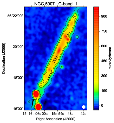
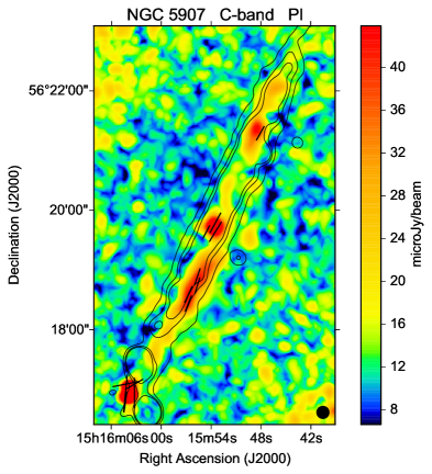
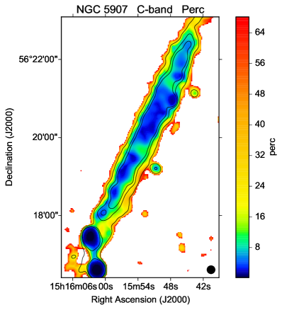
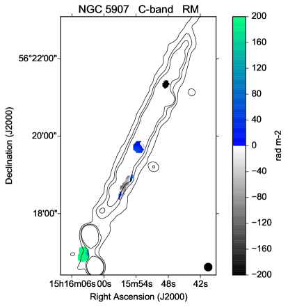
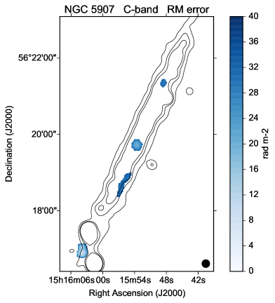
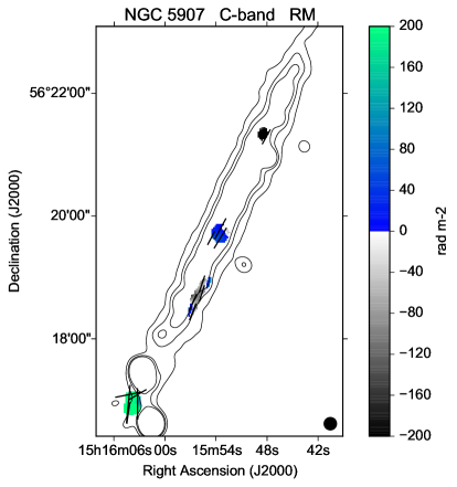
Figure 28: Polarization results for NGC 5907 at C-band and $12\hbox{${}^{\prime\prime}$}$ HPBW, corresponding to $980\,\rm{pc}$. The contour levels (TP) are 50, 150, and 250 $\mu$Jy/beam. The image of the TP map is cut at 1000 $\mu$Jy/beam in order to present the disk emission well. This just affects the two background sources in the south.

Maps of $\chi$ and $P$ (Eqns. 1 and 2) were made for each galaxy for the purpose of initial inspection. As a result of this exercise, 7 galaxies were excluded from the stacking process. These were: NGC 2992 (core/jets, see Irwin et al. 2017), NGC 4244 (no emission), NGC 4438 (core plus radio lobe only), NGC 4594, NGC 4845 and NGC 5084 (nuclear sources only), and UGC 10288 (dominated by a background double-lobed radio source, see Irwin et al. 2013). This left 28 galaxies for stacking. Each of these galaxies shows polarization in the disk although there is considerable structure in the polarization as Fig. 8 to Fig. 28 show. Because of this, we do not exclude galaxies that have known radio structures, such as radio lobes, associated with AGNs (e.g. NGC 4388 and NGC 3079). Such peculiarities could perturb an average map, but as long as disk and halo PI exist, the galaxy is included under the assumption that underlying disk- and halo-related polarization may still be present.

2.2 Galaxy Alignment and Angular Scaling

Table 1 provides galaxy distances, scaling and rotation data for the following discussion. Each image ($Q$ and $U$ maps both PB-corrected and PB-uncorrected) had to be rotated and scaled in angular size in preparation for stacking. However, since the polarization images tend to be complex, it was not possible to scale/rotate them based on the appearance of the polarization.

For this reason, the orientation (position angle) of a galaxy was initially taken from the K_s passband as given in the NASA Extragalactic Database (NED) but minor adjustments were made by eye (mostly zero but all $<$ 5 deg) to fine-tune the disk alignment so that the total intensity radio images aligned with the x axis.

We next wish to scale all galaxies to have the same angular size. Our argument for this scaling is based on the possibility that the underlying polarization structure could be self-similar as described by Henriksen et al. (2018). This means that galaxies of different size could still show (for example) X-type fields but on a scale appropriate to the galaxy. Without any such scaling, the 28 galaxies span a factor of 9 in angular size and we would not expect to see any polarization structures that are common to them all in a stacked image. A factor of 4 in angular size is due to differences in the physical sizes of the galaxies and the remainder is due to different distances.

For the angular scaling, we examined the 22 $\mu$m WISE (Wide-field Infrared Survey Explorer) images (Wright et al., 2010) with resolution enhanced to a final value of 12.4 arcsec via the WERGA process (Jarrett et al., 2012, 2013). Measured diameters are given in Wiegert et al. (2015, their Table 6). We therefore scale the angular sizes of all galaxies (their $Q$ and $U$ images) to match that of the largest galaxy, namely NGC 4244 which was 11.53 arcmin in diameter. Which size to adopt for the angular scaling is arbitrary, but by choosing the largest galaxy, we can ensure that all other galaxies become larger and no information is lost between pixels. In this process, we also scale the synthesized beam and ensure that the integrated flux density is conserved. That is, the galaxies are scaled in angular size but retain their original integrated flux densities.

Once all images have the same angular size, we have actually adjusted for two effects: differences in the physical sizes of the galaxies, and differences in their distances. For example, suppose two galaxies are at the same distance but of different physical size. In that case, if the smaller galaxy is scaled up to the larger size but retains its original integrated flux density as we have done, then its surface brightness will be lower. We take this as a reasonable approach to ’physical scaling’. On the other hand, suppose that a distant galaxy is scaled up in angular size as if it were a nearby galaxy. In that case, retaining the original integrated flux density as we have done is not correct and the integrated flux density should actually be increased to account for the closer distance. Therefore this ’distance scaling’ requires an adjustment to the integrated flux density which we will make a correction for in Sect. 2.4.

The rotated scaled images were finally converted to units of Jy/pixel and rescaled on a common grid. The PB for each galaxy was also scaled and rotated following the same procedure as above, and ensuring that the intensity value is 1.0 at the beam center. Rotation is necessary for the larger galaxies for which there were two pointings (NGC 891, NGC 3628, NGC 4565, NGC 4594, NGC 4631, and NGC 5907). PB Rotation is not strictly necessary for PBs of the single-pointing galaxies since the PB is symmetric but was carried out anyway for coding and header consistency.

Table 1: Scaling and Rotation of the Galaxies

Galaxy Key Distance ^a Angular Rotation ^c

for Fig. 2 Scaling ^b

[Mpc] [^∘]

NGC 660 28 12.3 3.82 49

NGC 891 10 9.1 1.21 66

NGC 2613 1 23.4 2.3 -24

NGC 2683 11 6.27 2.24 49

NGC 2820 20 26.5 6.48 25

NGC 3003 2 25.4 3.07 12

NGC 3044 12 20.3 3.76 -25

NGC 3079 21 20.6 2.66 -79

NGC 3432 3 9.42 3.18 48

NGC 3448 13 24.5 6.59 25

NGC 3556 22 14.09 1.90 9

NGC 3628 4 8.5 1.16 -14

NGC 3735 14 42 4.09 -40

NGC 3877 23 17.7 3.22 56

NGC 4013 5 16 3.34 24

NGC 4096 15 10.32 2.94 73

NGC 4157 24 15.6 3.14 27

NGC 4192 6 13.55 1.86 -62

NGC 4217 16 20.6 2.96 41

NGC 4302 25 19.41 3.02 -88

NGC 4388 7 16.6 5.01 1

NGC 4565 17 11.9 1.11 -44

NGC 4631 26 7.4 1.06 6

NGC 4666 8 27.5 2.86 50

NGC 5297 18 40.4 5.24 -59

NGC 5775 27 28.9 3.03 -56

NGC 5792 9 31.7 4.49 4

NGC 5907 19 16.8 1.57 -65

• Galaxy distance from Wiegert et al. (2015).

• Factor by which galaxies are scaled in size, based on their 22 $\mu$m diameters as given in Wiegert et al. (2015).

• Required counter-clockwise (=positive) rotation for x-axis alignment.

2.3 Galaxy Weighting

The PB-corrected images are required for stacking but, after scaling by angular size, each pixel corresponds to a different part of the PB from galaxy to galaxy. Consequently the rms noise at each pixel is different from galaxy to galaxy. Thus, we wish to weight each galaxy at a given pixel by the rms noise at that location. The weighting at any position is

$$W_{i}\,=\,\frac{1}{{\sigma_{i}}^{2}}$$ (3)

where $\sigma$ is the rms noise of the PB-corrected map at that position and $i$ refers to the galaxy. Also, the PB is cut off at 0.1 times the peak of 1.0 (which is at the map center) and any point that might fall outside of the cutoff must be set to zero and not counted in a weighted sum.

In order to compute $\sigma_{i}$, we measure the value of $\sigma_{i}$ of the PB-uncorrected scaled and rotated $Q$ and $U$ maps which have uniform noise, and divide the scaled and rotated PB by this noise value. This generates maps of $\sigma_{i}$ that increase with distance from the map center for each galaxy, $i$, as needed for Eqn. 3. We then form maps of $W_{i}U_{i}$ and $W_{i}Q_{i}$ for each galaxy, where $Q_{i}$ and $U_{i}$ have been rotated and scaled in angular size as described above. We also form a map of the sum of the weights, $\Sigma_{i}\,W_{i}$, for the purposes of normalization.

The weighted sum of the electric field vectors at any pixel is

$$\chi_{W}\,=\,\frac{1}{2}arctan\left[\frac{\Sigma_{i}\left(W_{i}U_{i}\right)}{\Sigma_{i}\left(W_{i}Q_{i}\right)}\right]$$ (4)

The weights, $W_{i}$ are the same for $Q_{i}$ and $U_{i}$ since the rms noise is approximately the same for the two maps at any position. Hence a normalization by the sum of the weights in the numerator and denominator of Eqn. 4 would cancel and is not required. Note that Eqn. 4 supercedes Eqn. 1.

2.4 Polarization Weighting and Scaling for Distance

We now have a series of galaxy $Q$ and $U$ images that have been scaled in angular size and weighted by rms noise, but their integrated flux densities retain their original values as explained in Sect. 2.2. To correct for this, we now scale these flux densities by distance. To accomplish this, we scaled each map to the distance of the closest galaxy which is NGC 4244 at a distance of 4.4 Mpc (see Footnote 6), that is, we apply a scaling for galaxy, $i$, of $(D_{i}/4.4)^{2}$ for $D$ in Mpc, as given in Table 1. We finally form the weighted sum of this ‘polarization luminosity’ for any pixel according to

$${Q_{W}}\,=\,\frac{\Sigma_{i}\,\left[\left(\frac{D_{i}}{4.4}\right)^{2}W_{i}Q_{i}\right]}{\Sigma_{i}W_{i}},\leavevmode\nobreak\ \leavevmode\nobreak\ \leavevmode\nobreak\ \leavevmode\nobreak\ \leavevmode\nobreak\ \leavevmode\nobreak\ \leavevmode\nobreak\ \leavevmode\nobreak\ {U_{W}}\,=\,\frac{\Sigma_{i}\,\left[\left(\frac{D_{i}}{4.4}\right)^{2}W_{i}U_{i}\right]}{\Sigma_{i}W_{i}}$$ (5)

$$P_{W}\,=\,\sqrt{{Q_{W}}^{2}\,\,+\,{U_{W}}^{2}}$$ (6)

Note that Eqn. 6 supercedes Eqn. 2. The final map showing $P_{W}$ in colour and $\chi_{W}$ as vectors (rotated by 90 degrees to represent magnetic field orientations) is shown in Fig. 1. All final quantities are in units of Jy/pixel.

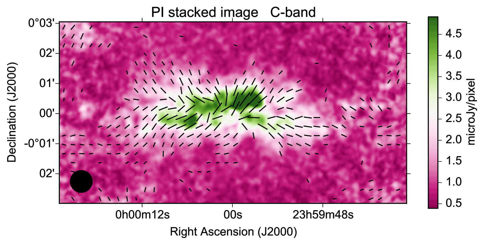
Figure 1: Weighted mean linear polarization (in colours), scaled to a common angular size (11.5 arcmin) and to a common distance (4.4 Mpc), which correspond to NGC 4244. The horizontal extent of the image shown is 11.5 arcmin, or 14.8 kpc at the common distance. The average scaled synthesized beam is shown as a circle at lower left. Vectors show the orientation of the weighted scaled apparent magnetic field. Note their ‘X-shaped’ orientation.

2.5 Checks for Dominant Galaxies

Before discussing the results of Fig. 1 we need an additional check to see whether the stacking has strongly favoured one or two galaxies in comparison to all others. In other words, could a galaxy be so dominant that the stacking simply highlights the structure of that one galaxy? To check this, we compute maps of scaled weighted Q and U for each galaxy individually and then compute the average Q and U for each galaxy. For this calculation, there are no sums over galaxies in Eqn. 5 so the calculation is determined from, $Q_{W_{i}}\,=\,(D_{i}/4.4)^{2}\,W_{i}\,Q_{i}$ and $U_{w_{i}}\,=\,(D_{i}/4.4)^{2}\,W_{i}\,U_{i}$. For the average of the region shown in Fig. 1, we then plot the result in Fig. 2, presented as a log plot in order to see each galaxy more clearly. Since the plot is a diagnostic intended for comparison between galaxies only, we have first multiplied $Q_{W_{i}}$ and $U_{w_{i}}$ by a constant for a simpler reading of the y-axis scale. Finally, since $Q_{W_{i}}$ and $U_{w_{i}}$ can be positive or negative, we must take the log of the absolute value and then have restored the negative to the result.

Fig. 2 shows that the individual galaxies vary in $Q$ and $U$ over several orders of magnitude. Since the average of Fig. 1 is a linear average, it is possible that only the peaks (either positive or negative) strongly contribute to the average. However, various galaxies dominate, depending on what parameter is considered. For example, the most dominant galaxies in positive Q are NGC 3628, NGC 4631, while the most dominant galaxies in negative Q are NGC 891 and NGC 4302. The most dominant galaxies in positive U are NGC 3628, NGC 4565, and NGC 4631, and those in negative U are NGC 2683, NGC 4217, and NGC N3079. If we repeat this exercise with a more restrictive field, then these dominant galaxies tend to change. For example, NGC 4565 becomes the dominant galaxy in positive Q, depending on where the measurement is made. Moreover, NGC 4565 does not show a particularly impressive halo or X-type field (Appendix A).

We conclude that the stacked image shown in Fig. 1 to be discussed in the next section is, to the limitations of our data, a realistic description of a ’mean’ magnetic field.

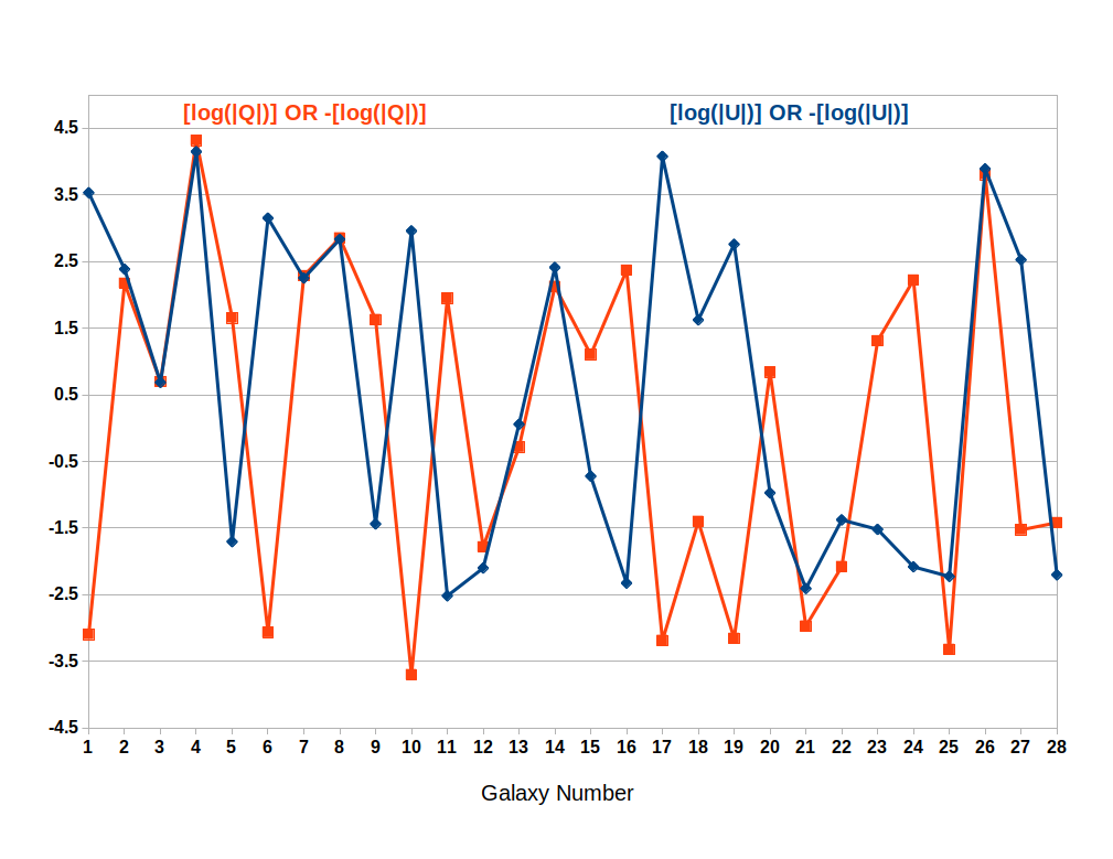
Figure 2: Scaled and weighted Q (red curve) and U (blue curve) for each galaxy individually. See Sect. 2.5 for a description. The numbers on the x-axis indicate the galaxies according to the Key given in Table 1.

2.6 Stacking results

Fig. 1 displays the result of our polarization stacking at C-band. The displayed horizontal size is approximately equal to the scaled 22 $\mu$m size of our galaxies (11.53 arcmin). Our first conclusion is that the region over which polarization occurs in the galaxies is smaller than the 22 $\mu$m galaxy size. This is likely a signal-to-noise (S/N) issue since linear polarization is weaker than total intensity. The complexity of the emission is also evident. There remain AGNs in the sample, some of which have radio lobes (e.g. NGC 3079, NGC 4388) and this may contribute to the irregularity in the brightness.

The overall structure of the stacked apparent magnetic field vectors is indeed X-shaped, with vectors more parallel to the galactic midplane along the disk (best visible in the western part of the disk), as expected from an inclined plane-parallel spiral disk field. Note that the effects of Faraday rotation and depolarization (which are uncorrected in these C-band data) are expected to be strongest along the disk and inner halo. This explains why the stacked apparent magnetic field vectors look most regular in the outer parts of the halo and the polarized intensity is slightly weaker along the thin galaxy disk direction (horizontal line at DEC = 0 deg). In a sense, it is surprising that any structure is seen at all in the stacked magnetic field. If we recall that $Q$ and $U$ can be positive or negative, the sums in Eqn. 4 might have resulted in zero or, at least, a random field orientation. The fact that X-type structure is visible in a sum of 28 galaxies argues in favour of the scale invariance that was assumed in Sect. 2.2.

Fig. 1 shows some scattered emission to the far right and left of the main emission region. This is largely due to the fact that some galaxies have companions or strong background sources in the field that were not excised prior to stacking. This introduces a discussion as to alternate methods of stacking the images. One might have excised such emission prior to the stacking, for example. We have retained any radio lobe structure near AGNs (e.g. NGC 3079) and have also retained any background sources that might be seen through the disk (e.g. two background sources at the far end of the disk of NGC 5907). A future approach might be to subtract such known sources in advance. Another approach is to do the angular scaling according to the total intensity radio continuum emission extent, rather than according to the $22\mu$m emission size. Even the rotation could be honed so that the x-axis alignment is oriented with all advancing sides together and all receding sides together. A future effort could do a more complete search through parameter space. If the result improves, this could lead to more insight as to what is actually driving the X-types (or other) structures. Therefore, we consider our result to be a first step.

In spite of these caveats, it is remarkable that coherent polarization structure remains when the $Q$ and $U$ maps are weighted and scaled as described above. Although not perfect, the X-shaped structure of the magnetic field can indeed be seen in the stacked image, arguing for self-similarity as described in Henriksen et al. (2018) with axially symmetric fields as the dominant mode.

3 RM-synthesis

3.1 Parameters and polarization imaging

We performed RM-synthesis (Brentjens & de Bruyn, 2005) for each of our 35 CHANG-ES galaxies at C-band and L-band. The image cubes in Stokes Q and U were prepared in the following way: at C-band we defined 16 spectral windows, corresponding to a frequency spacing of 128 MHz and $\lambda^{2}$ spacings between $0.7\,\rm{and}\,1.7\,\rm{cm}^{2}$. To obtain a similar $\lambda^{2}$ range at L-band, each spectral window (among 29 in total) was split into 4 sections of 13 channels each, assuming that the edge-channels 0 - 5 and 58 - 63 are always flagged. This corresponds to a frequency spacing of 3.25 MHz within each spectral window and 6 MHz between spectral windows, or $\lambda^{2}$ spacings between $0.85\,\rm{and}\,2.7\,\rm{cm}^{2}$.

As a first step, the CASA task $statw$ was run on each individual data set, to make sure all visibilities have the correct weighting when combining different array configurations. For each of the frequency intervals specified above, the $clean$ task was run on Stokes Q and U of the polarization calibrated data sets of the combined C- and D-array configurations at C-band and B-, C-, and D-array configurations at L-band. The pixel size was chosen to be $1.5\hbox{${}^{\prime\prime}$}$ with an image size of 600 x 600 at C-band (720 x 720 for galaxies with two pointings) and 2400 x 2400 at L-band. We used the multi-frequency synthesis (MFS) with nterms = 1 and used a maximum of 2000 clean components that were mostly sufficient to reach our stopping threshold of $25\,\mu\mathrm{Jy/beam}$ at C-band and $300\,\mu\mathrm{Jy/beam}$ at L-band, usually corresponding to 2 - 4 times the noise rms of the clean images. For all maps we used natural weighting (robust = 2) in order to be more sensitive to extended faint emission, without applying any uv tapering. The maps were convolved to a common beam size of $12\hbox{${}^{\prime\prime}$}$, primary-beam corrected, and concatenated into a single data cube file, each for Q and U.

These data cubes were used as input for the RM-synthesis code (Heald et al., 2009) to produce the Faraday cubes in Q, U, and Faraday depth ($\phi$). With our spectral windows we cover a range in Faraday depth between $+8192\,\mathrm{rad/m}^{2}$ and $-8192\,\mathrm{rad/m}^{2}$ with channel separations of $64\,\mathrm{rad/m}^{2}$ at C-band and between $-2048\,\mathrm{rad/m}^{2}\leq\phi\leq+2048\,\mathrm{rad/m}^{2}$ with channel separations of $8\,\mathrm{rad/m}^{2}$ at L-band.

The Faraday spectra were cleaned down to a $3\,\sigma$-noise level of the uncleaned Q and U cubes using the algorithm by Heald et al. (2009), extended by Adebahr et al. (2017). These cleaned Q and U Faraday cubes were used to estimate the polarized intensity PI pixel wise. PI is not corrected for Ricean bias. We finally determined a PI map, consisting of the maximum value along the PI cube for each pixel in RA-DEC space, a map of the peak RM which for each pixel corresponds to the $\phi$ value at which the maximum in the PI cube occurs. Further, a map of the observed polarization angle was computed at each position from the Q and U values in the $\phi$ plane where the maximum in the PI cube occurs. The RM and polarization angle maps were computed in regions where PI is higher than 5 times the noise rms in the clean Faraday Q and U image planes where the (Ricean) bias in the polarized intensity only plays a minor role.

The observed polarization angles were Faraday rotation corrected with the corresponding RM values and the corresponding central wavelength in order to receive a map of the intrinsic polarization angles PA. In addition, the RM maps have been corrected for their Galactic foreground contribution RM_fg which was determined from the Galactic RM map of Oppermann et al. (2012) at the position of each galaxy (see Table 2). We also calculated the error maps of the PI, RM, and PA maps.

Table 2: Foreground Rotation Measure $\mathrm{RM_{fg}}$, distances, linear resolutions that correspond to $12\hbox{${}^{\prime\prime}$}$, and range of observed RMs observed at C-band in the disk and/or halo of the galaxies

Galaxy $$RM_{\mathrm{fg}}$$ distance lin. res.@12^′′ RM_disk/halo range remarks

[] [Mpc] [pc] []

NGC 660 12.3 720 -204 to 330 polar ring galaxy

NGC 891 9.1 530 -209 to 466

NGC 2613 23.4 1360 -328 to 242

NGC 2683 6.3 360 PI too weak

NGC 2820 26.5 1540 -173 to 156

NGC 2992 34.0 1980 central source only

NGC 3003 25.4 1480 PI too weak

NGC 3044 20.3 1180 -238 to 372

NGC 3079 20.6 1200 -331 to 239 strong central source

NGC 3432 9.4 550 PI too weak

NGC 3448 24.5 1430 -232 to 217

NGC 3556 14.9 820 -226 to 362

NGC 3628 8.5 490 -339 to 319 strong central source

NGC 3735 42.0 2440 -216 to 249

NGC 3877 17.7 1030 PI too weak

NGC 4013 16.0 930 -248 to 163

NGC 4096 10.3 600 PI too weak

NGC 4157 15.6 910 -422 to 255

NGC 4192 13.6 790 -184 to 263

NGC 4217 20.6 1200 -179 to 189

NGC 4244 4.4 260 no polarization at all

NGC 4302 19.4 1130 -287 to 214

NGC 4388 16.6 970 -164 to 295 nuclear outflow

NGC 4438 10.4 600 core plus radio lobe only

NGC 4565 11.9 690 -204 to 342

NGC 4594 12.7 740 central source only

NGC 4631 7.4 430 -551 to 823

NGC 4666 27.5 1600 -190 to 358

NGC 4845 17.9 990 central source only

NGC 5084 23.4 1360 -49 to 322 central source only

NGC 5297 40.4 2350 PI too weak

NGC 5775 28.9 1680 -271 to 335

NGC 5792 32.7 1840 PI too weak

NGC 5907 16.8 980 -152 to 126

UGC 10288 34.1 1980 background radio source only

• See CHANG-ES VII paper (Damas-Segovia et al., 2016)

• See CHANG-ES V paper (Irwin et al., 2015)

• See CHANG-ES III paper (Irwin et al., 2013)

3.2 Results and Faraday depolarization

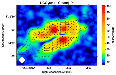
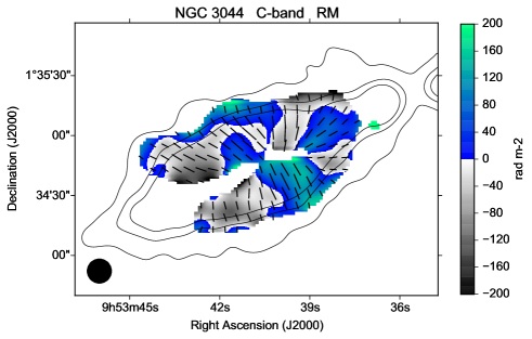
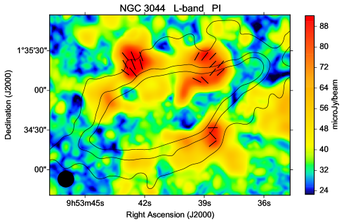
Figure 3: Polarized intensity (left) and Rotation Measure (right) of the spiral galaxy NGC 3044 at C-band (5 - 7 GHz) (upper panels) and L-band (lower panels) with a resolution of $12\hbox{${}^{\prime\prime}$}$ HPBW presented within the same field on the sky. The vectors are corrected for the observed Faraday rotation at the corresponding frequency band which give the intrinsic magnetic field orientation at C-band. The contours indicate the total intensity at 50, 150, and 250 $\mu$Jy/beam at C-band and 125, 375, and 625 $\mu$Jy/beam at L-band, corresponding to $5\,\sigma$, $15\,\sigma$, and $25\,\sigma$ r.m.s. each.

We discuss NGC 3044 as an example galaxy first, before presenting the others. The resultant maps of the linear polarization (PI) and RM of the NGC 3044 are shown in Fig. 3 for C-band in the upper panels and for L-band in the lower panels. At C-band the linear polarization is observable within most parts along the disk and the halo. It is concentrated within the $25\,\sigma$ contours of total intensity. There is only a thin area along the central and eastern disk of the galaxy without linear polarization. At L-band, the distribution of the polarized intensity looks completely different: The peaks in PI are located far away from the disk in the outer halo of NGC 3044, while the projected galactic disk and inner halo are completely depolarized.

The observed RM values in NGC 3044 are very different at both frequency bands: at C-band more than 99% of the values are in the range between $+200\,\mathrm{rad/m}^{2}$ and $-200\,\mathrm{rad/m}^{2}$ (max$=372\,\mathrm{rad/m}^{2}$, min$=-238\,\mathrm{rad/m}^{2}$) while at L-band they are in a the small range between $+24\,\mathrm{rad/m}^{2}$ and $-14\,\mathrm{rad/m}^{2}$. These RM ranges should be similar in a source without Faraday depolarization. Also the magnetic field vectors corrected for the observed RM at the corresponding frequency band also look somehow different at L-band when compared to those at C-band. In general, the vectors at C-band show a very smooth, regular structure, while those in two of the three blobs at L-band look rather irregular.

All these findings strongly indicate that the L-band data are strongly affected by Faraday depolarization and even completely depolarized over large areas in NGC 3044. Faraday depolarization can be caused by thermal electrons together with a regular magnetic field within the emitting source (differential Faraday rotation) and/or by random magnetic fields within the source (internal Faraday dispersion) or between the source and the observer (external Faraday dispersion) (Burn, 1966; Sokoloff et al., 1998). From the observations of a smooth, large-scale pattern in RM at C-band together with the regular pattern of the magnetic field vectors, we conclude that the magnetic field in NGC 3044 is regular (see Sect. 4). Hence, we expect differential Faraday depolarization in NGC 3044.

RM-synthesis can be used to identify the effects of differential Faraday depolarization, however, it is unable to recover emission that is completely depolarized by this process. A first complete depolarization by differential Faraday rotation at L-band occurs already around $RM\approx\pm 40\,\mathrm{rad/m}^{2}$ for the mid frequency of the observed total band while at C-band this occurs at a much larger value around $RM\approx\pm 630\,\mathrm{rad/m}^{2}$ at the mid frequency (Arshakian & Beck, 2011, their Eq. 4). While the observed RM values in NGC 3044 at C-band are below the range of complete differential Faraday depolarization, they are far above the value at L-band. This indicates that the observed polarized intensity at L-band is depolarized over wide ranges along the line of sight. This means that NGC 3044 is Faraday thick at L-band along its disk and huge parts of its halo while the galaxy is Faraday thin at C-band in the entire halo. There is just a thin depolarization lane along parts of the galactic disk of NGC 3044 where the thermal electrons and also the total magnetic field strength are expected to be highest.

NGC 3044 is just an example for the strong depolarization at L-band. Generally, we find that the observed RM values at L-band are in the range $+50\,\mathrm{rad/m}^{2}$ and $-50\,\mathrm{rad/m}^{2}$, hence limited by strong Faraday depolarization which means that they are Faraday thick over wide areas of their halos if they host large-scale magnetic fields. Only the observed RM values at C-band are below the range of complete differential depolarization. They can be regarded as a reliable tracer of the parallel magnetic field component along the whole line-of-sight of the galaxy, especially outside the midplane where the thermal electron density is expected to be largest. Hence, we only used the C-band data for our further analysis.

After RM-synthesis, the vectors are corrected for the observed RM and the Galactic foreground rotation measure $\mathrm{RM_{fg}}$ (see Sect. 3.1) and hence are the intrinsic magnetic field vectors.

When analyzing the C-band D-array maps we detected polarized intensity PI in each of the 35 CHANG-ES galaxies except in NGC 4244. This galaxy is extremely faint even in total intensity (TP) with values of $\lesssim 12\,\mu$Jy/beam as extended emission at 12^′′ HPBW. Hence we cannot expect to observe any PI from NGC 4244 with the sensitivity of our survey. In addition, seven other galaxies show extended PI that is $\lesssim 40\,\mu$Jy/beam for which our RM-synthesis with the parameters given in Sect. 3.1 does not give any polarization vectors or RM values. These galaxies are: NGC 2683, NGC 3003, NGC 3432, NGC 3877, NGC 4096, NGC 5297, and NGC 5792. These 7 galaxies are, however, included in the stacked PI image of Fig. 1. In 5 other galaxies (NGC 2992, NGC 4438, NGC 4594, NGC 4845, and NGC 5084) the polarized intensity is dominated by the strong emission of the central source and no polarization can (clearly) be ascribed to the disk/halo emission. The same is valid for UGC 10288 where the polarized intensity originates from a background double-lobed radio source (Irwin et al., 2013). These latter 6 galaxies were also excluded from the stacked PI image (Fig. 1) and will not further be discussed here. Instead, they will be published in a separate CHANG-ES paper.

Altogether, we are left with a sample of 21 spiral galaxies with significant linear polarization for which the CHANG-ES observations allowed for the first time to determine reliable RM-values in galactic halos.

We present the polarization results at C-band for these 21 galaxies in Fig. 8 to Fig. 28 . Each galaxy is presented on a separate page with six panels. They contain: total intensity (TP, Stokes I) with contours at 5, 15, 25 $\sigma$ r.m.s. and intrinsic polarization vectors (upper left, panel 1), polarized intensity (PI) with intrinsic polarization vectors and the contours of TP as given in panel 1 (upper right, panel 2), percentage polarization (referred to as Perc in the Figures) with TP contours of panel 1 (mid left, panel 3), rotation measure (RM) with TP contours of panel 1 (mid right, panel 4), errors in RM with TP contours of panel 1 (lower left, panel 5), rotation measure with intrinsic polarization vectors and TP contours of panel 1 (lower right, panel 6). The total intensity maps show the observations at C-band D-array only, while the polarization maps are made from C-band, D- and C-array combined as described in Sect. 3.1. The maps in the 6 panels for each galaxy are equal in size given by the extent of the total emission (5 $\sigma$ r.m.s.) and are centered on the nucleus of the galaxy. All maps have an angular resolution of 12^′′ and are corrected for the primary beam. The latter leads to an increase of the r.m.s. noise towards the map edges which is visible in some of the images, especially those that are observed with two pointings (given in Sect. 2.2). Corresponding high values at the edges of the PA, RM- and RM error maps were excluded. In the percentage map, values $\leq 0\%$ and $\geq 70\%$ are excluded as they are unphysical. The TP contours of panel 1 are presented in all panels of each galaxy to serve as orientation. The length of the intrinsic magnetic field vectors is proportional to PI at this position.

Similar to NGC 3044, the majority of the intrinsic RM-values of our sample galaxies are in the range between $+200\,\mathrm{rad/m}^{2}$ and $-200\,\mathrm{rad/m}^{2}$. The RM ranges found within the disk and halo (i.e. excluding other areas) are explicitly given in Table 2 for all galaxies. NGC 4631 is the galaxy with the highest RM values, comparable to the values found by Mora & Krause (2013). These high values are mainly found along the disk and disk/halo interface of NGC 4631 and are related to the high thermal electron density there (Mora-Partiarroyo et al., 2019a, b).

Though the polarized intensity is in general quite weak in some parts of the galaxies presented in Fig. 8 to Fig. 28, it leads to remarkable percentage polarization within the outer contours of total intensity in all galaxies. This will be discussed in Sect. 5. The intrinsic magnetic field vectors and RM values are only given in those areas where PI is larger than about $40\,\mu\mathrm{Jy/beam}$, due to the cut-off levels used for RM-synthesis as explained in Sect. 3.1.

4 Large-scale magnetic fields

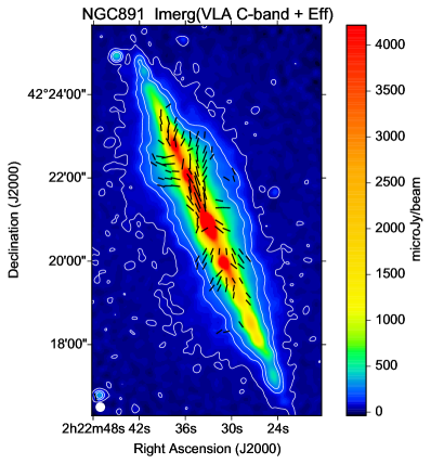
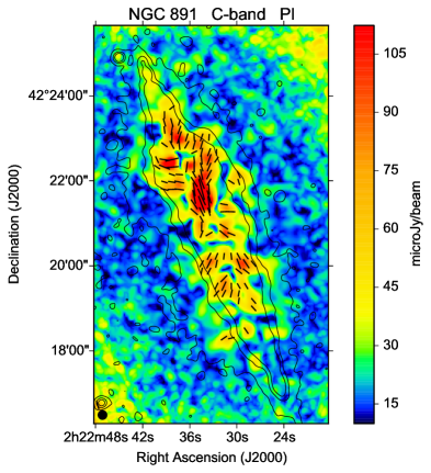
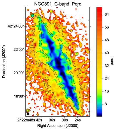
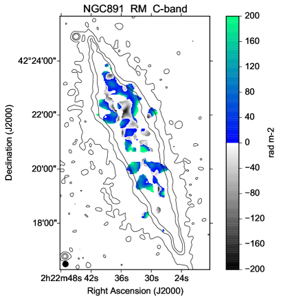
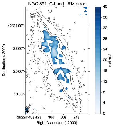
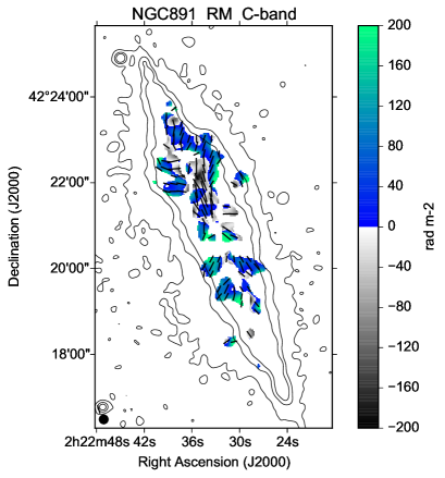
Figure 9: Polarization results for NGC 891 at C-band and $12\hbox{${}^{\prime\prime}$}$ HPBW, corresponding to $530\,\rm{pc}$. The contour levels (TP) are 50, 150, and 250 $\mu$Jy/beam.

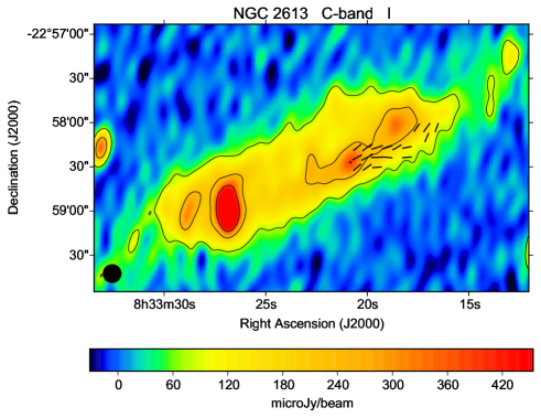
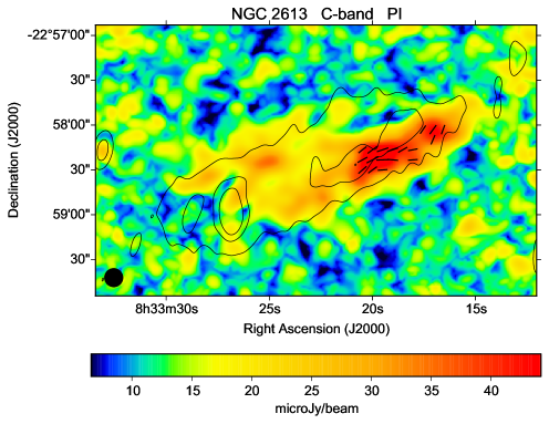
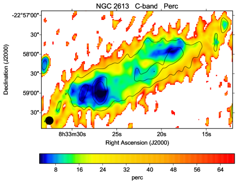
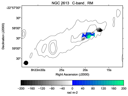
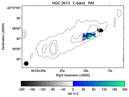
Figure 10: Polarization results for NGC 2613 at C-band and $12\hbox{${}^{\prime\prime}$}$ HPBW, corresponding to $1360\,\rm{pc}$. The contour levels (TP) are 75, 225, and 375 $\mu$Jy/beam.

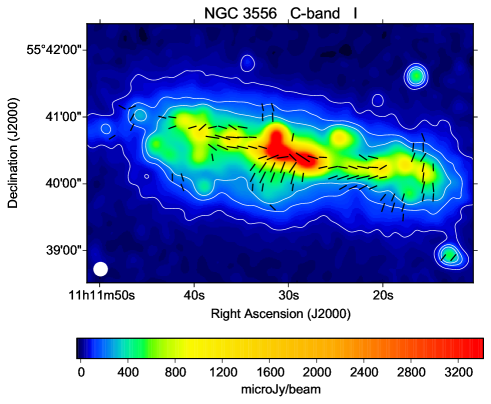
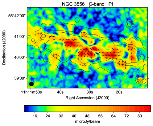
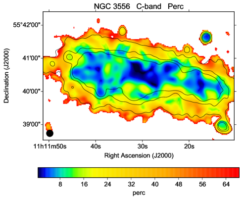
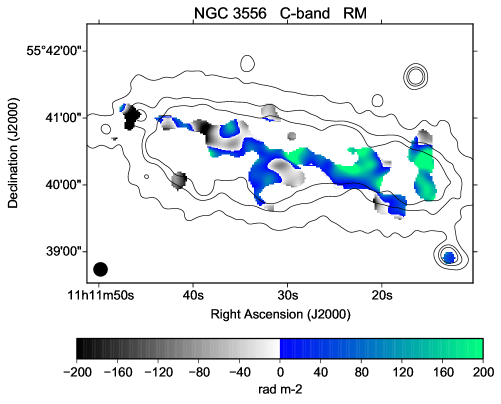
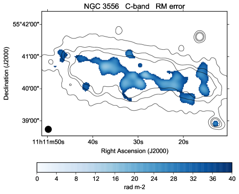
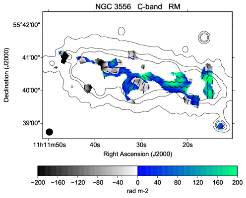
Figure 15: Polarization results for NGC 3556 at C-band and $12\hbox{${}^{\prime\prime}$}$ HPBW, corresponding to $820\,\rm{pc}$. The contour levels (TP) are 50, 150, and 250 $\mu$Jy/beam.

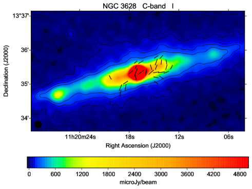
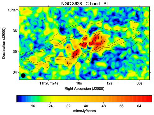
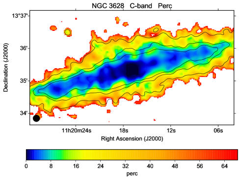
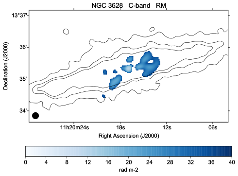
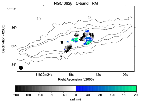
Figure 16: Polarization results for NGC 3628 at C-band and $12\hbox{${}^{\prime\prime}$}$ HPBW, corresponding to $490\,\rm{pc}$. The contour levels (TP) are 50, 150, and 250 $\mu$Jy/beam. The image of the TP map is cut at 5000 $\mu$Jy/beam in order to present the disk emission well.

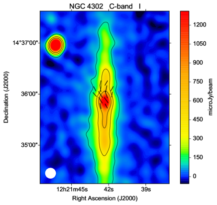
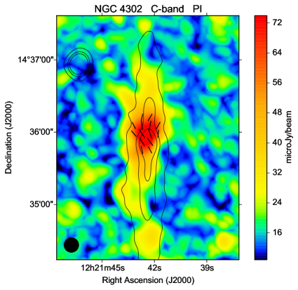
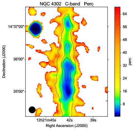
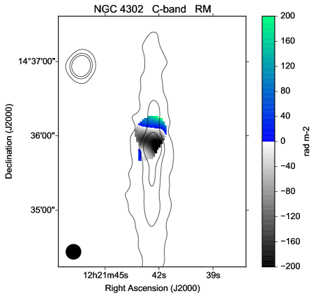
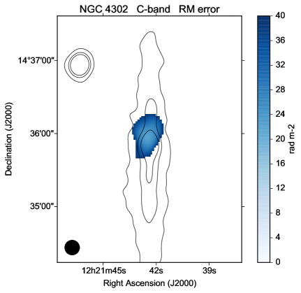
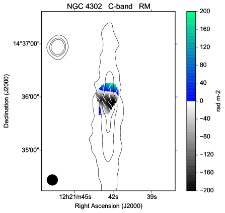
Figure 22: Polarization results for NGC 4302 at C-band and $12\hbox{${}^{\prime\prime}$}$ HPBW, corresponding to $1130\,\rm{pc}$. The contour levels (TP) are 100, 300, and 500 $\mu$Jy/beam.

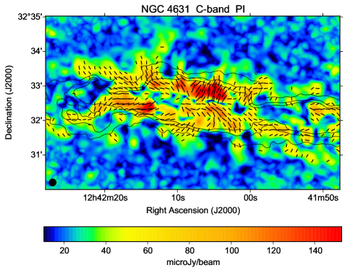
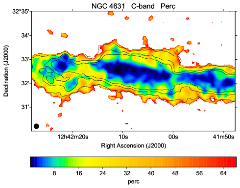
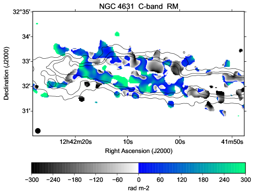
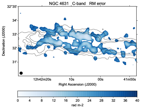
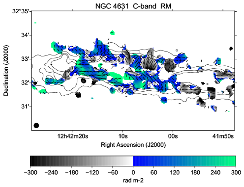
Figure 25: Polarization results for NGC 4631 at C-band and $12\hbox{${}^{\prime\prime}$}$ HPBW, corresponding to $430\,\rm{pc}$. The contour levels (TP) are 75, 225, and 375 $\mu$Jy/beam.

The majority of the 21 galaxies presented in Fig. 8 to Fig. 28 show intrinsic magnetic field vectors within a significant part of their halos and/or projected disks as summarized in Table 3. This is not the case only for four of these galaxies, namely NGC 2613, NGC 3628, NGC 4302, and NGC 5907. The reason is for NGC 2613 (Fig. 10), NGC 4302 (Fig. 22), and NGC 5907 (Fig. 28) that they are too faint in linear polarization within most parts of their halos/disks, while NGC 3628 (Fig. 16) has, in addition, a strong central source. The intrinsic magnetic field orientations exhibit a regular and smooth pattern in 14 of the remaining 17 galaxies. Only NGC 891 (Fig. 9), NGC 3556 (Fig. 15), and NGC 4631 (Fig. 25) show a more patchy structure in their intrinsic magnetic field vectors.

Table 3: Magnetic field angles and RM pattern analysis

regular more patchy only visible in small areas

NGC 660 NGC 891$$\,{}^{\mathrm{a,b}}$$ NGC 2613

NGC 891 NGC 3556 NGC 3628

NGC 2820 NGC 4631 NGC 4302

NGC 3044 NGC 5907

NGC 3079

NGC 3448

NGC 3735

NGC 4013

NGC 4157

NGC 4192

NGC 4217

NGC 4388

NGC 4565

NGC 4631

NGC 4666

NGC 5775

• at $20\hbox{${}^{\prime\prime}$}$ HPBW (corresponding to 880 pc)

• at $12\hbox{${}^{\prime\prime}$}$ HPBW (corresponding to 530 pc)

• at $20\hbox{$.\!\!^{\prime\prime}$}5$ HPBW (corresponding to 730 pc)

• at $12\hbox{${}^{\prime\prime}$}$ HPBW (corresponding to 430 pc)

A smooth pattern of the intrinsic magnetic field vectors may indicate a large-scale magnetic field but can also originate from anisotropic random magnetic fields, e.g., compressed fields with reversing directions. However, as anisotropic random magnetic fields have different directions along the line of sight (LoS), the differential RMs along the LoS have different signs and at least partly cancel each other. Only the detection of RMs of reasonable strengths along the LoS indicates a regular magnetic field component. If, in addition, the different RM observed along different LoS presented in a map have a smooth distribution of regions with positive and negative RM values on scales significantly larger than the beam size, a regular (coherent) magnetic field is indicated. In this case, the intrinsic polarization vectors are also expected to be ordered on scales larger than the synthesized beam size.

Remarkably, in all these areas of regular magnetic field vectors in the galaxies mentioned above, we also find significant RM values that vary smoothly and show the same sign over huge areas when compared to the telescope’s beam of $12\hbox{${}^{\prime\prime}$}$ HPBW. This already indicates a regular magnetic field component parallel to the LoS. The RM values in the Figures are presented in two different color wedges, one for positive RM values (blue-green), and one for negative RM values (gray-scale). This makes it easier to distinguish between the different magnetic field directions. The errors in RM are between a few and $40\,\mathrm{rad/m}^{2}$, and much smaller than most of the observed RMs. Hence, the observed large-scale changes of sign in RM are real and can only be interpreted as a change of the direction of the parallel component of the regular magnetic field in the corresponding regions of the galaxy. Altogether, we conclude that we detected coherent magnetic fields in the halos of our sample spiral galaxies.

In three galaxies the magnetic field vectors and RM values could only be detected along the projected disk. These are NGC 5907 and NGC 4013 (see also Stein et al. (2019b)), and also probably NGC 4565 (see Schmidt et al. 2019) where we detect magnetic field vectors and RM values only up to about 1.0 kpc distance from the midplane. For the other galaxies, the distances from the midplane up to which the large-scale magnetic field could be detected, are given in Table 4. As they are measured in the sky plane, they are lower limits. However, with the inclination $i\geq 75\hbox{${}^{\circ}$}$ of our CHANG-ES galaxies, their deprojected values may only be larger by 10% at most. We stress that these values are limited by the sensitivity of our polarization observations (and the cut levels we used for a reliable RM-synthesis) and hence are smaller than the physical extent of the large-scale fields in the halo.

Table 4: Large-scale magnetic fields in the halo

source vertical RMTL$$\,{}^{\mathrm{b}}$$ magnetic field RMTL Hubble type SFR

detection orientation

[kpc] [kpc]

NGC 660 1.7 SBa 3.3

NGC 891 2.5 Sb 1.9

NGC 2820 2.9 yes horizontal 2.0 SBc 1.4

NGC 3044 3.3 yes vertical 2.2 SBc 1.8

NGC 3079 4.9 SBcd 5.1

NGC 3448 2.7 possible possibly vertical S0-a 1.8

NGC 3556 2.5 SBc 3.6

NGC 3735 4.6 possible horizontal Sc 6.2

NGC 4157 2.5 yes horizontal 2.2 SABb 1.8

NGC 4192 1.3 yes horizontal 1.3 SABb 0.8

NGC 4217 3.1 yes horizontal 2.4 Sb 1.9

NGC 4388 2.4 Sb 2.4

NGC 4631 2.8 yes vertical 1.9 SBcd 2.6

NGC 4666 5.3 SABc 10.5

NGC 5775 5.4 Sbc 7.6

• in the sky plane

• Rotation measure transition line

• Projected distance between RMTLs

• From HYPERLEDA, as used in Irwin et al. (2012)

• this is SFR_revised in Vargas et al. (2019)

• In the northern half (as detected in Mora-Partiarroyo et al. 2019b)

It remains the question why NGC 4631 does not show such a smooth, regular pattern in the magnetic vectors and RM values in Fig. 25 though this galaxy has been reported recently to show large-scale magnetic field reversals (Mora-Partiarroyo et al., 2019b). These authors presented the same polarization observations with an angular resolution of $20\hbox{$.\!\!^{\prime\prime}$}5$, while the maps in Fig. 25 are made with $12\hbox{${}^{\prime\prime}$}$ HPBW. At the distance of NGC 4631, $12\hbox{${}^{\prime\prime}$}$ HPBW correspond to 430 pc while $20\hbox{$.\!\!^{\prime\prime}$}5$ correspond to 740 pc. For comparison, all maps of NGC 4631 with a resolution of $20\hbox{$.\!\!^{\prime\prime}$}5$ are presented again in our notations in Fig. 4. And indeed, at this linear resolution of about 800 pc also NGC 4631 shows a smooth and regular pattern in the magnetic field vectors as well as in the RMs. This example indicates that the larger-scale coherent magnetic field component in NGC 4631 has typical scales larger than about 800 pc, and is accompanied by a smaller-scale magnetic field component. As soon as the resolution is better than the scale of the coherent magnetic field, we start to resolve the smaller-scale magnetic field and hence reduce the uniformity of the vectors and the RM pattern.

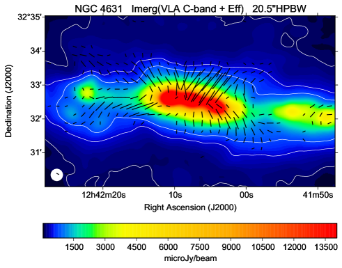
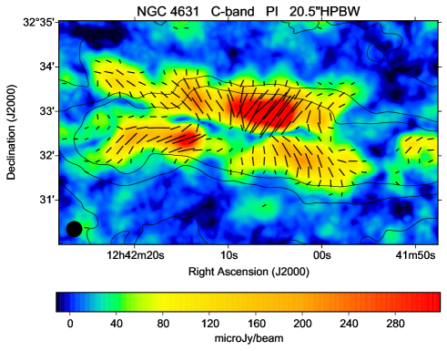
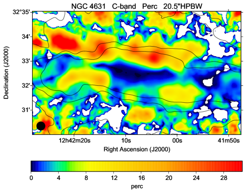
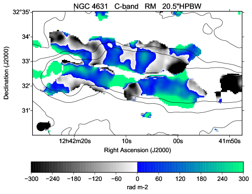
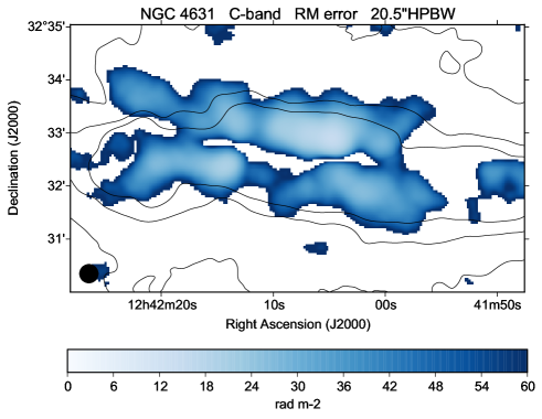
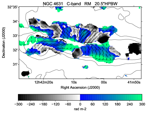
Figure 4: Polarization results for NGC 4631 at C-band and 20 $.\!\!^{\prime\prime}$5 HPBW. The contour levels (TP) are 150, 450, and 750 $\mu$Jy/beam.

Though the galaxies are presented with the same angular resolution ($12\hbox{${}^{\prime\prime}$}$ HPBW), the detected linear polarization corresponds to different linear scales for each single galaxy due to their different distances. These distances are listed in Table 2, leading to linear resolutions between 260 pc (for NGC 4244) and 2.44 kpc (for NGC 3735) for the angular resolution of $12\hbox{${}^{\prime\prime}$}$  HPBW.

Also NGC 891 shows a patchy structure at scales larger than the HPBW of $12\hbox{${}^{\prime\prime}$}$ (corresponding to 530 pc) in their magnetic field vectors and their RM values, although it was referred to as a kind of prototype of an X-field structure by observations at the 100-m telescope at Effelsberg at much lower resolution of $84\hbox{${}^{\prime\prime}$}$  HPBW (Krause, 2009). Again, we smoothed our Q- and U-cubes to $20\hbox{${}^{\prime\prime}$}$ HPBW (corresponding to 880 pc) before RM-synthesis. The corresponding results are presented in Fig. 5. The magnetic field angles as well as the RM-values show again a more regular pattern that is not only due to a higher signal-to-noise in the smoothed maps. This is best visible in the RM-maps (panel 4 and panel 5) in the central part of NGC 891.

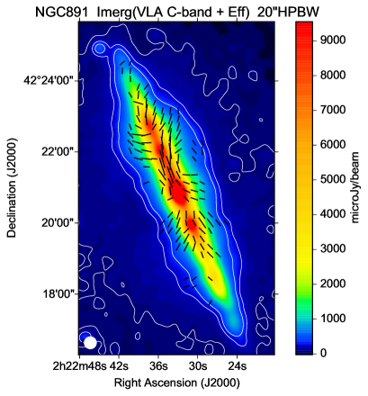
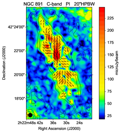
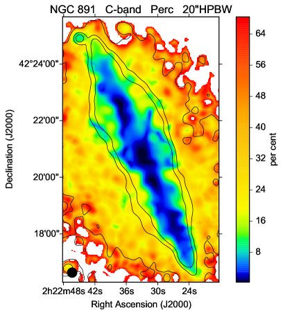
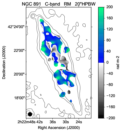
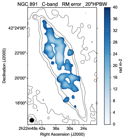
Figure 5: Polarization results for NGC 891 at C-band and $20\hbox{${}^{\prime\prime}$}$ HPBW. The contour levels (TP) are 75, 225, and 375 $\mu$Jy/beam.

Nevertheless, the global structure in NGC 891 is still somewhat patchy even at 880 pc linear resolution. There is also NGC 3556 observed near the detection limit that shows a somewhat patchy pattern. This galaxy has a linear resolution of 820 pc, hence comparable to NGC 891 at $20\hbox{${}^{\prime\prime}$}$ HPBW. Also NGC 3556 may look more regular at a lower angular resolution which in this case may also be due to a higher signal-to-noise ratio.

To quantify the relative importance of angular scales, we applied wavelet transformations to the maps in polarized intensity of NGC 891 and NGC 4631 at $12\hbox{${}^{\prime\prime}$}$ HPBW,following Frick et al. (2016). We used ‘Texan Hat’ functions that provide a higher resolution in spatial frequency space than ‘Mexican Hat’ functions. The wavelet power spectra are shown in Fig. 6. The smallest scale of $a=4$ corresponds to the HPBW of $12\hbox{${}^{\prime\prime}$}$. The power spectra show two prominent peaks. The first ones are located at small scales of $22\,\hbox{${}^{\prime\prime}$}$ ($\approx$ 970 pc) and $18\,\hbox{${}^{\prime\prime}$}$ ($\approx$ 670 pc) in NGC 891 and NGC 4631, respectively. These scales represent structures of the magnetic field smaller than the large-scale coherent field, but clearly larger than the telescope resolution. The second peaks in the power spectra are located at scales of about $1.5\,\hbox{${}^{\prime}$}$ ($\approx$ 4 kpc) and $3.8\,\hbox{${}^{\prime}$}$ ($\approx$ 8 kpc) in NGC 891 and NGC 4631, respectively, are due to the large-scale polarized emission from the disk.

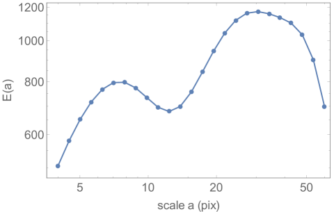
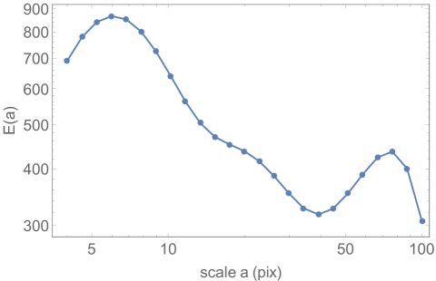
Figure 6: Wavelet power spectra of the maps of polarized intensity ($PI$) at C-band for NGC 891 (left panel) and for NGC 4631 (right panel) at $12\hbox{${}^{\prime\prime}$}$ HPBW. Scale $a$ is the scale of the wavelet function in pixelsize ($1\hbox{$.\!\!^{\prime\prime}$}5$) which is half of the size of the structure in the map (see text for details). $E(a)$ is the energy density of thewavelet transform on scale $a$.

It is striking that we detect a smooth pattern in the magnetic field angles and the RMs only in galaxies with a linear resolution corresponding to scales larger than about 700 pc. Hence we conclude that the large-scale (coherent) magnetic fields in the halos have typical scales of about 1 kpc or larger.

With our present observations we can trace the magnetic field vectors and RMs up to about 10 kpc (mean value $5\pm 2$ kpc) distance from the midplane of the disk (see Table 4), hence far into the halo. The intrinsic magnetic field vectors give the orientation of the large-scale (coherent) magnetic field component within the sky plane (perpendicular magnetic field component), while the RMs give the magnetic field component along the line of sight (parallel magnetic field component) of the large-scale magnetic field. Unfortunately, they are averaged along the long line of sight through the disk and halo in edge-on galaxies. Though RM-synthesis partly corrects for differential depolarization, it can only be done ’on average’ along the line of sight. This makes it difficult to identify the 3-dimensional structure of the large-scale magnetic field from the observations.

Our observations do not indicate a simple, large-scale magnetic field pattern in the halo like a dipole or quadrupole structure as expected by dynamo models. They also do not exhibit a systematic single sign change of RM across the minor axis as would be expected for large-scale toroidal halo fields. The field patterns seem to be more complicated. Only the RMs give the magnetic field direction of the parallel magnetic field component, while the ’vectors’ just give the orientation of the perpendicular magnetic field components. At the transition line between positive and negative RMs (i.e. where the parallel magnetic field component changes its direction) we observe that the perpendicular magnetic field components occur at any angles in our maps.

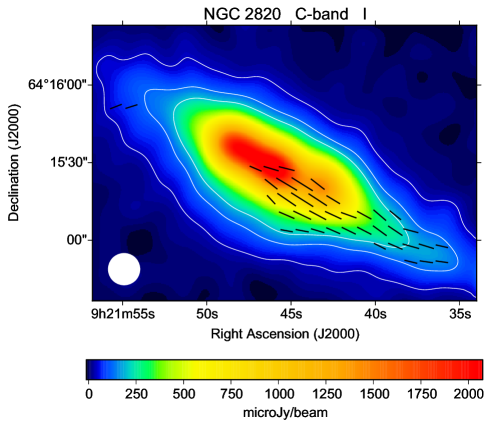
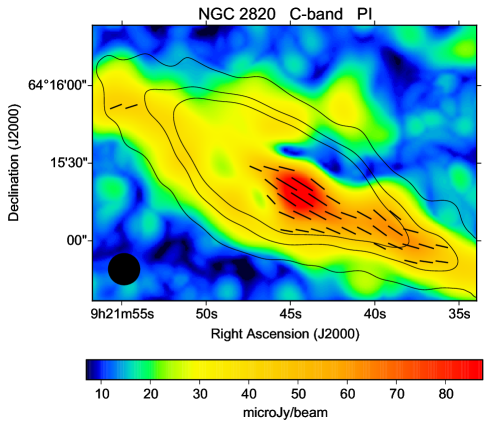
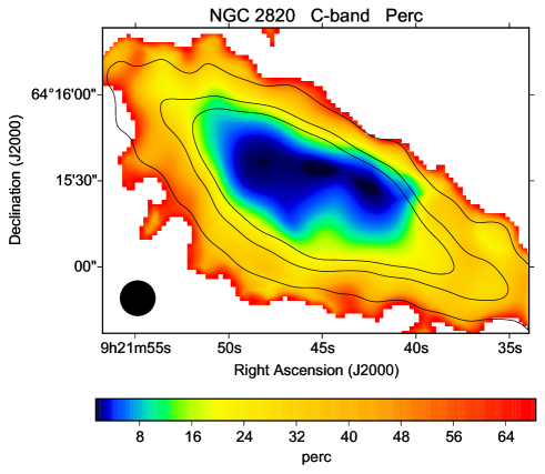
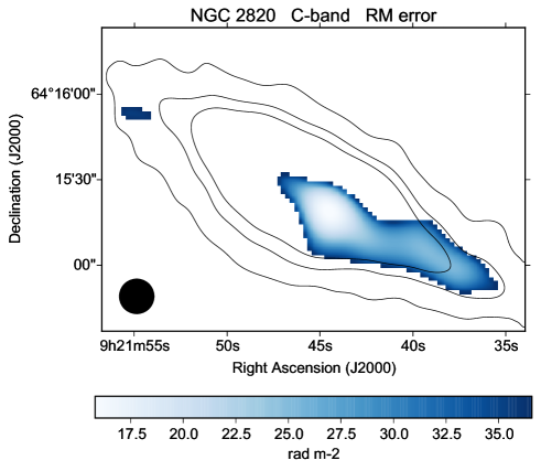
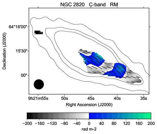
Figure 11: Polarization results for NGC 2820 at C-band and $12\hbox{${}^{\prime\prime}$}$ HPBW, corresponding to $360\,\rm{pc}$. The contour levels (TP) are 40, 120, and 200 $\mu$Jy/beam.

These RM-transition lines (RMTL) themselves show an interesting vertical pattern in NGC 4631 as detected by Mora-Partiarroyo et al. (2019b): they are vertical to the galactic plane, indicating several periodic large-scale field reversals in the northern halo of NGC 4631 (see Fig. 4). The intrinsic magnetic field vectors have only small angles with respect to the RM-transition lines there. As presented and discussed in Mora-Partiarroyo et al. (2019b) the observations indicate giant magnetic ropes (GMR) rising perpendicular from the northern galactic disk into the halo (see their Fig. 7). In our sample galaxies we find another five (possibly seven) galaxies with vertical RM transition lines (see Table 4). In two of them (NGC 3044 and NGC 3448) the magnetic field vectors are also oriented nearly in parallel with these lines. We conclude that NGC 3044 is another galaxy with GMR extending far into its halo. NGC 3448 can be considered as a candidate for GMR which needs to be confirmed by more sensitive polarization observations. In the remaining four (possibly five) galaxies with vertical RM-transition lines, we find magnetic field vectors that are orientated roughly perpendicular to the RM-transition lines (best visible in NGC 2820 in Fig. 11).

We estimated the projected distances between the vertical RM-transition lines ($\Delta$ RMTL) parallel to the major axis. The values are about 2 kpc (see Table 4).

5 Degree of polarization and the ordered magnetic field

We determined the degree of polarization (P$=\rm{PI/TP}\cdot 100$) for our sample galaxies. This quantity may be affected by missing large-scale flux density as expected in TP for galaxies that are larger than $4\hbox{${}^{\prime}$}$ in extent at C-band. As PI is usually structured on smaller scales, it is expected to be less or barely affected by missing spacings.

For three of the large galaxies, NGC 891, NGC 4565 and NGC 4631, we used the VLA TP maps that were merged with Effelsberg 100-m single dish observations at 6 cm, as described in Schmidt et al. (2019) for NGC 891 and NGC 4565, and Mora-Partiarroyo et al. (2019a) for NGC 4631. Most of the other galaxies are smaller than $4\hbox{${}^{\prime}$}$ in TP at C-band and are tested to show no indication of obvious missing spacing problems (Krause et al., 2018). Only four other galaxies in our sample are larger than 4^′ at C-band: NGC 3556, NGC 3628, NGC 4192, and NGC 5907. We do not have single-dish observations for them. Hence, their degree of polarization may be affected by missing spacings in TP and can be regarded as upper limits.

Values for which P is $<0\%$ and $\gtrsim 70\%$ are unphysical and appear in map areas with low signal-to-noise ratios. Hence, they are excluded. The resultant maps of the degree of polarization are presented in panels 3 of Fig. 8 to Fig. 28 for each galaxy.

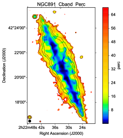
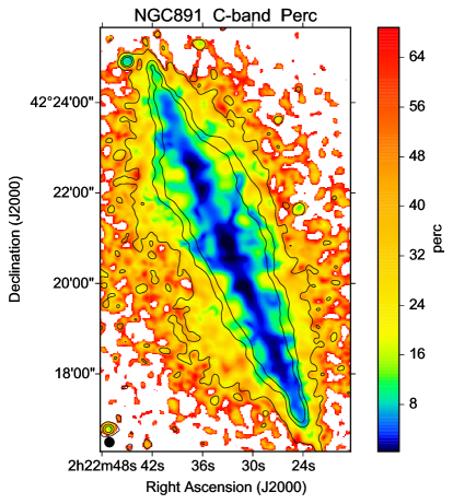
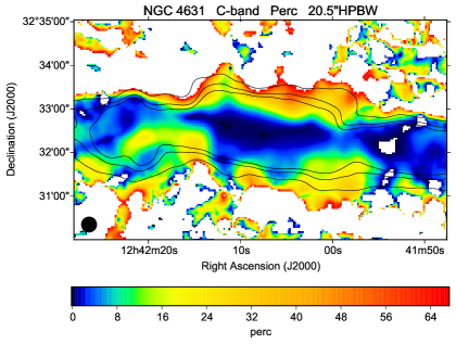
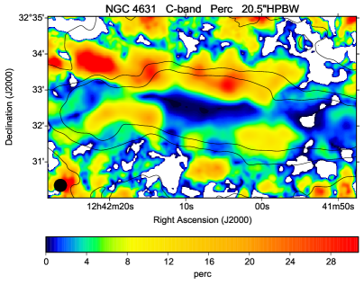
Figure 7: Degree of polarization at C-band for NGC 891 at $12\hbox{${}^{\prime\prime}$}$ HPBW (upper panels) and for NGC 4631 at $20\hbox{$.\!\!^{\prime\prime}$}5$ HPBW (lower panels) with VLA-data only (left panels) and VLA and 100-m Effelsberg data merged in TP (right panels). The contours indicate the total intensity at $5\,\sigma$, $15\,\sigma$, and $25\,\sigma$ r.m.s. of the corresponding TP.

We observe that the degree of polarization increases monotonically from the galactic midplane towards the outer boundaries of the halo for all galaxies, except for NGC 4631 at $20\hbox{$.\!\!^{\prime\prime}$}5$ HPBW. We estimated the mean values for P in the area where TP is between $5\,\sigma$ and $15\,\sigma$ r.m.s for all galaxies. They are very similar for these galaxies with values in the range of about $10\%<\rm{P}<40\%$ there, with the highest values near the outer edges of the galaxies. This large-scale increase of the degree of polarization cannot be explained just by a vertical decrease of the thermal fraction of the disk as the decrease is also observed far in the upper halo. This can only be explained by a vertical increase of the degree of alignment of the magnetic field. This means that the scale height of the ordered magnetic field is larger than that of the total magnetic field and that the ordered magnetic fields extend far out in the halo and beyond.

This observational result is fully consistent with what follows from the assumption of energy equipartition between the magnetic field and the nonthermal electrons as usually applied for the magnetic field strength estimate (Beck & Krause, 2005)). The assumption of equipartition implies $N_{CR}\propto B^{2}$ with $N_{CR}$ being the total number density of cosmic ray particles. This leads to a scale length of the ordered magnetic field $l_{B}=2\,l_{CR}$, hence $l_{B}\simeq 4\,h_{syn}$ (see Krause 2019).

The only different distribution in P is observed in NGC 4631 at $20\hbox{$.\!\!^{\prime\prime}$}5$ HPBW with the merged TP map. There, the degree of polarization increases with distance from the galactic midplane up to about $35\%$ at a vertical distance of 2 kpc but decreases again at larger distances from the midplane. This is different to the other galaxies. Some of those with a smaller angular extent (hence without large-scale missing flux densities) like NGC 3735 or NGC 5775 show a P that can be traced in vertical direction up to 8 kpc or 10 kpc and P is still monotonically increasing. Also the merged version of NGC 891 shows a vertical monotonically increasing degree of polarization up to distances of 5 kpc.

It is unclear yet what causes the different appearance of NGC 4631, and whether it is real. NGC 4631 has been observed with two pointings along its major axis. The polarized intensity in panel 2 Fig. 4 decreases upwards of about 2 kpc ($1\hbox{${}^{\prime}$}$) above the midplane, but then seems to increase again at the upper boundary of the map. This increase is probably artificial and due to the increasing noise due to the primary beam correction that had been applied to the maps. On the other hand, this is in the area where the TP is significant only in the merged map (compare panel 1 in Fig. 4 with that in Fig. 25) and may hence be less reliable. We conclude that the large vertical extent of the halo in NGC 4631 requires observations with more pointings in vertical direction to give reliable values for the degree of polarization. Only then we can decide whether NGC 4631 also needs a correction for large-scale missing polarized flux density. This would imply that the large-scale polarization structure and hence the ordered magnetic field in NGC 4631 would be more extended than about 8 kpc.

6 Discussion

The most striking result from the polarization stacking is that the stacked (apparent) magnetic field vectors reveal an underlying ‘X-shaped’ structure as described in Sect. 2. The 28 galaxies that were used for stacking are of very different Hubble types, with different star formation activities in their disks, and at locations from being rather isolated to various interacting phases. The X-shaped structure has been seen in various individual galaxies in the past but the results of this polarization stacking appear to show that this structure is an underlying feature of many and likely most galaxies. This result also indicates scale invariance of the polarization structure. Even the distribution of the stacked polarized intensity seems to form an X-shaped structure similar to the observation of NGC 4631 alone as visible in Fig. 4.

We like to stress that the vectors in Fig. 1 are apparent magnetic field vectors that are not corrected for Faraday rotation. The largest effect of Faraday rotation is expected in the midplane, decreasing from the inner halo outwards to negligible values. This is also reflected in Fig. 1 in the way that the vectors in or near the midplane look less regular than further out. It may explain why we do not observe plane-parallel vectors along the central midplane of the stacked image as is expected for a plane-parallel magnetic field structure as observed in most of the disks of spiral galaxies seen face-on. Though, a plane-parallel field is indicated along the outer western midplane of the stacked image.

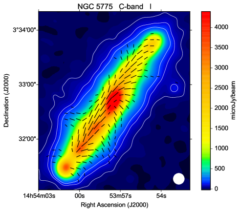
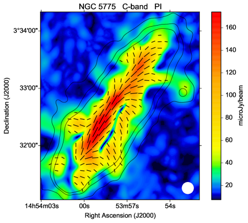
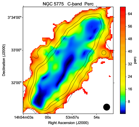
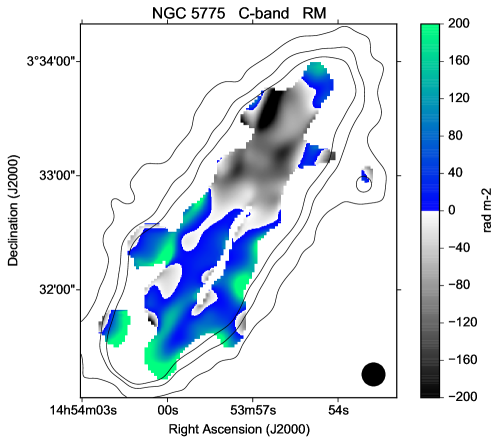
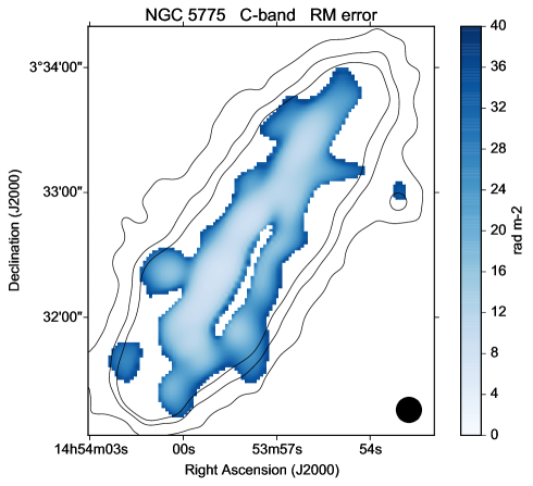
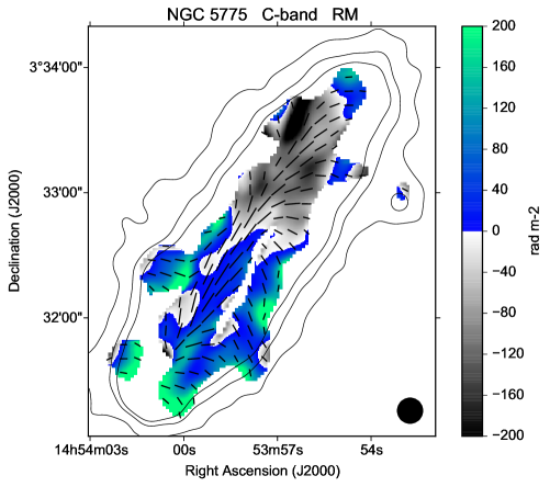
Figure 27: Polarization results for NGC 5775 at C-band and $12\hbox{${}^{\prime\prime}$}$ HPBW, corresponding to $1680\,\rm{pc}$. The contour levels (TP) are 35, 105, and 175 $\mu$Jy/beam.

The magnetic field vectors in the maps of the individual galaxies (Fig. 8 to Fig. 28) are corrected for Faraday rotation, hence give the intrinsic magnetic field orientation averaged along the whole line of sight through the galaxy. They are not less regular along the midplane and in most cases reveal a plane-parallel disk-field in projection. In some galaxies there are thin lines without polarized intensity along the galactic disk as in NGC 4631 (Fig. 4, panel 2) and in NGC 5775 (Fig. 27, panel 2). In these cases we see, different to our general assumption in Sect. 3.2, that even at C-band some galaxies are Faraday thick along some parts of their disk planes due to high thermal electron densities there. This has been extensively discussed for NGC 4631 in Mora & Krause (2013).

The decrease of the polarized intensity at the outer areas of the galaxies, however, is related to the decrease in synchrotron emission, as it is accompanied by the decrease in total intensity. As the scale length of the ordered magnetic field is much larger than that of synchrotron emission (as discussed in Sect. 5) it means that the decrease of (polarized) radio intensity is mainly due to the decrease in number density of the relativistic electrons in the halo or their energy losses by radiation. With more sensitive receivers or longer integration times we could probably observe galactic halos to much further extents.

Considerable theoretical effort has been put into models of dynamo action to explain regular halo fields (e.g. Sokoloff & Shukurov, 1990; Brandenburg et al., 1993; Moss et al., 2010; Henriksen et al., 2018, and references therein) that look X-shaped when observed. A current summary can be found in Moss & Sokoloff (2019) and Beck et al. 2019 (GALAXIES). A galactic outflow is included in many of these models. This is no unrealistic constraint as the existence of galactic winds has been reported for many of the CHANG-ES galaxies (Krause et al., 2018; Miskolczi et al., 2019; Stein et al., 2019a; Schmidt et al., 2019; Mora-Partiarroyo et al., 2019a), and extraplanar ionized gas emission can be seen in many H$\alpha$ images taken for the CHANG-ES sample (Vargas et al., 2019).

NGC 4631 was the first galaxy in which a large-scale magnetic field in the halo was detected (Mora-Partiarroyo et al., 2019b). It even shows periodic large-scale field reversals in its northern halo (see Fig. 4) which can be modeled by accretion models of the scale-invariant mean-field dynamo theory (Woodfinden et al., 2019). Vertical RM-transition lines (RMTL) have been detected in at least six galaxies of our sample (as described in Sect. 4). One of them, NGC 3044, exhibits Giant Magnetic Ropes (GMR) as detected in NGC 4631. Similar to the latter, NGC 3044 shows indications for a strong disturbance, like e.g. by a past merger (Zschaechner et al., 2015). Also NGC 3448 shows indications of GMRs.

The large-scale magnetic fields in the other 4 galaxies with vertical RMTL are mainly horizontally orientated. These could possibly be explained by ’GMR’ that spiral with rather tightly wound lines, either upwards from or downwards to the galactic disk through the halo along cylinders with a diameter given by $\Delta$ RMTL. We call them horizontal GMRs. The vertical GMRs observed in NGC 3044 and NGC 4631 could eventually be understood as part of very loosely wound helices. Model simulations are necessary to test these ideas.

We noticed an asymmetry in the distribution of the polarized intensity in the disk and halo: PI is usually stronger in one half of the galaxy along the major axis than in the other. In order to quantify the asymmetry, PI was integrated on both sides of the major axis in boxes extending out to the weakest emission in vertical direction (Table 4) and in radial direction. The bright polarized emission from the lobes of NGC 3079 and NGC 4388 is not related to the large-scale magnetic fields in the disk or halo and hence was subtracted before the integration. Polarized background sources, not related to the galaxies, were found, one in each of the fields of NGC 3735, NGC 5775, and NGC 5907, and were subtracted, too.

The asymmetry is measured by the parameter $q=(A-R)/(A+R)$ where $A$ and $R$ are the integrated polarized flux densities on the approaching and the receding sides, respectively. $q=0$ means no asymmetry, $q=\pm 1$ maximum asymmetry (one side missing completely). The accuracy of the $q$ measurements was tested by slightly varying the integration boxes and was found to be about 20%.The $q$ values are given in Table 5. $q$ is positive in 13 out of 18 galaxies, with values ranging between 0.047 and 0.275, while four galaxies show negative values. In one galaxy (NGC 4631) no significant asymmetry can be measured. The probability that the preference of positive $q$ values is by chance is estimated as $(17!\,/\,(13!4!))\,/\,2^{17}\cdot 100=1.8\,\%.$

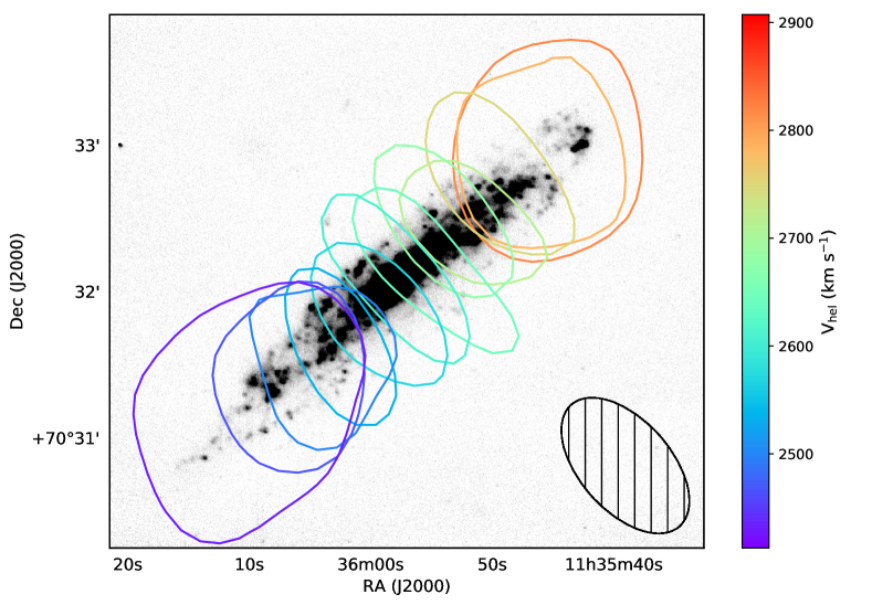
Figure 29: HI contour map of NGC3735 on top of its grey-scale H$\alpha$ map (Vargas et al. 2019). The contours are plotted at the 3 mJy/beam level, from every even channel in the HI cube, such that purple-blue colours correspond to the approaching side and orange-red colours correspond to the receding side. The velocity range is about 2380-3000 km/s. The synthesized beam is shown in the bottom right, and is 66.9x37.4 arcsec, with PA=41.8 deg.

We compared this PI asymmetry with the overall rotation of the galactic disk by determining the approaching side of the major axis from observed velocities in HI or CO. These values were found in the literature for all galaxies except for NGC 3735. For this galaxy we reduced HI data observed with the VLA and determined a velocity map of NGC 3735 as described and shown in Fig. 29 in Appendix B . It shows that the south eastern side is the approaching one. The results are summarized in Table 5. Most of the galaxies presented in this paper show the strongest PI in C-band on the side of the major axis that is approaching with respect to the galaxy’s global rotation. This was first recognized in NGC 4666 by Stein et al. (2019a).

Table 5: Global rotation and ordered magnetic field in the halo

Galaxy Side with Approaching Asymmetry $$q$$ Reference

strongest PI side of

in disk+halo major axis

NGC 660 NE NE 0.246 van Driel et al. (1995)

NGC 891 NE NE 0.147 Garcia-Burillo & Guelin (1995)

NGC 2613 NW NW 0.101 Chaves & Irwin (2001)

NGC 2820 SW SW 0.100 Kantharia et al. (2005)

NGC 3044 NW NW 0.047 Lee & Irwin (1997)

NGC 3079 NW NW 0.275 Irwin & Seaquist (1991)

NGC 3448 SW NE -0.131 Noreau & Kronberg (1986)

NGC 3556 SW NE -0.042 King & Irwin (1997)

NGC 3735 SE SE 0.198 this paper

NGC 4157 SW SW 0.110 Verheijen & Sancisi (2001)

NGC 4192 NW NW 0.087 Cayatte et al. (1990)

NGC 4217 NE NE 0.106 Verheijen & Sancisi (2001)

NGC 4388 E W -0.192 Oosterloo & van Gorkom (2005)

NGC 4565 SE SE 0.055 Neininger et al. (1996)

NGC 4631 similar W 0.011 Wielebinski et al. (1999)

NGC 4666 NE NE 0.130 Walter et al. (2004)

NGC 5775 SE NW -0.124 Irwin (1994)

NGC 5907 SE SE 0.084 Dumke et al. (1997)

The asymmetry in C-band is of similar sign but weaker compared to that observed in L-band in mildly inclined galaxies of the SINGS survey (Braun et al., 2010). These authors explained the asymmetry by the superposition of a large-scale axisymmetric spiral field in the disk and a large-scale quadrupolar field in the halo. The asymmetry arises if only the near side of the galaxy is visible in polarized emission due to strong Faraday depolarization. The strength of the detected PI does not directly depend on the total ordered field strength (B_t) but on the strength of its perpendicular magnetic field component. Hence, PI depends on our viewing angle onto the magnetic field and its observed asymmetry may give important information about the large-scale structure of the regular field. The model by Braun et al. (2010) may also apply to edge-on galaxies observed in C-band with smaller but still significant Faraday depolarization. Refined model calculations for edge-on galaxies are needed.

An alternative model was proposed by Stein et al. (submitted to A&A) where the trailing spiral arms may explain the asymmetry in the disk and its correlation with the galactic rotation if the polarized emission from the near side of the galaxy dominates. However, a large fraction of the polarized emission in our sample galaxies emerges from the halo that does not host spiral arms. We hope that our comprehensive polarization study of edge-on galaxies triggers more theoretical efforts.

As noted Sect. 1, the galaxies of the CHANG-ES sample are of various Hubble types and star formation rates (SFR). The determination of reliable SFRs in edge-on galaxies is more difficult than in face-on galaxies and has recently been reexamined by Vargas et al. (2019). We present these values for the galaxies with an observed large-scale magnetic field in the halo in Table 4. There is no indication found that the existence of a large-scale magnetic is preferentially observed for galaxies with certain Hubble types or special SFR values.

Many of the CHANG-ES galaxies have been or are currently interacting with other galaxies (like the polar ring galaxy NGC 660) or are members of the Virgo cluster (like NGC 4192, NGC 4388, and NGC 4438) and we still detected large-scale halo magnetic fields in many of them. This indicates that a large-scale magnetic field - if once generated - cannot be destroyed easily and persists. Hence, it should be considered whether large-scale halo fields can be regarded as a link to intergalactic magnetic fields.

7 Summary and conclusions

In this paper we used two different approaches (stacking and RM-synthesis) to analyze the magnetic fields in the halo of spiral galaxies. We present a stacked image (C-band D-array configuration) of the linear polarization and apparent magnetic field vectors of all CHANG-ES galaxies that show polarization in their disks. These are 28 galaxies of very different Hubble types, star formation and interaction activities. The result is shown in Fig. 1. The striking result is that it clearly reveals an underlying X-shaped structure of the apparent magnetic field which seems to be an underlying feature of many and likely most spiral galaxies.

Secondly, we performed RM-synthesis on combined array configurations at C-band and at L-band of all 35 CHANG-ES galaxies and argue that only the C-band results can be regarded as a reliable tracer of the intrinsic magnetic field in the disk and halo. Polarized intensity was detected in all but one of the 35 galaxies. The outlier is NGC 4244 which is too faint, even in total power.

In seven galaxies of the sample, the polarized emission is detected but their signal-to-noise is too low for a reliable RM-synthesis (as described in Sect. 3.2). In six other galaxies, the polarized emission is clearly dominated by the central source or a background radio galaxy (UGC 10288) without clear polarized disk/halo emission. In total, we are left with 21 spiral galaxies that show extended polarized intensity within their disks and/or halos and for which the CHANG-ES observations allowed for the first time to determine reliable RM-values in galactic halos.

The resulting maps are presented in Fig. 8 to Fig. 28. Our main results are:

• We detected a regular, large-scale magnetic field in the halo of 16 galaxies.

• The scale of the regular magnetic field in the halo is typically 1 kpc or larger, while it extends over several kpc.

• While all these galaxies show large-scale magnetic field reversals with respect to the line of sight, we observed that these magnetic field reversals occur where the field in the plane of the sky extends approximately perpendicular to the galactic midplane (vertical RMTL, see Table 4) in six galaxies.

• In four of these six galaxies, the vertical RMTL have magnetic field vectors perpendicular to the lines. Only NGC 3044 and possibly NGC 3448 have the magnetic field vectors roughly parallel to these lines, similar to NGC 4631. Hence we detected at least one more galaxy with giant magnetic ropes (GMR) as defined in Mora-Partiarroyo et al. 2019b. The magnetic field vectors in the other four galaxies are mainly horizontally orientated.

• We observed an asymmetry in the distribution of the polarized intensity (PI) on both halves of the galaxy with respect to the minor axis. We found that the strongest PI is on the side of the major axis that is approaching with respect to the galaxy’s global rotation. PI depends on our viewing angle onto the magnetic field and its observed asymmetry may give important informations about the large-scale structure of the regular field.

• The degree of polarization increases monotonically from the galactic midplane towards the outer boundary of the halo. This implies that the scale height of the ordered magnetic field is larger than that of the total magnetic field and that the ordered (and probably also the regular) magnetic fields extend far out in the halo and beyond.
  

Altogether, we showed that large-scale (coherent) magnetic fields are common in the halos of spiral galaxies. Our observations do not indicate a simple, large-scale magnetic field pattern in the halo like a dipole or quadrupole structure as expected by $\alpha-\Omega$ mean-field dynamo models for the disk. They also do not exhibit a systematic single sign change of RM across the minor axis as would be expected for large-scale toroidal halo fields. The field patterns seem to be more complicated.

With more sensitive observations at C-band, we expect to detect these magnetic fields also in the halos of those galaxies whose signal-to-noise ratio are currently too low to detect extended RM and intrinsic magnetic field vectors. From our experience, we conclude that C-band is the best suited frequency band in terms of sensitivity and depolarization for a polarization study of galactic halos in nearby spiral galaxies. The best angular resolution for future observations is the one that corresponds to about 1 kpc in the galaxies, respectively.

We also observed large-scale magnetic field reversals with respect to the line of sight indicating giant magnetic ropes (GMR) that may be more or less tightly wound and extend far out in the halo. We anticipate that this discovery will strengthen the impact of large-scale dynamo theories for spiral galaxies. The regular halo fields may also be regarded as a link to intergalactic magnetic fields (see e.g. Henriksen & Irwin 2016) and could help to understand their origin which is still a mystery.

Appendix A Polarization maps with RM-synthesis

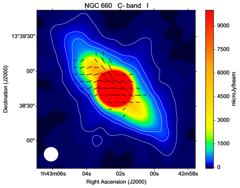
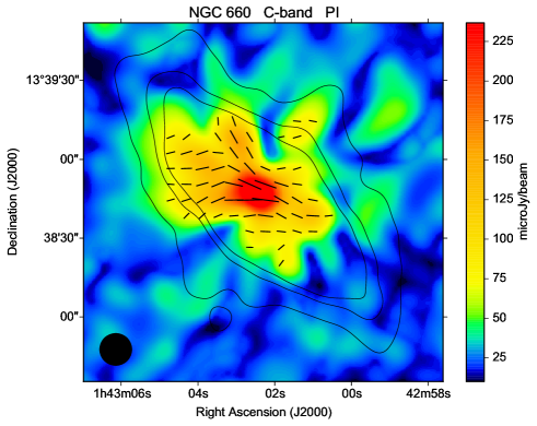
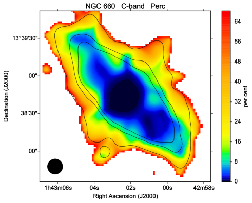
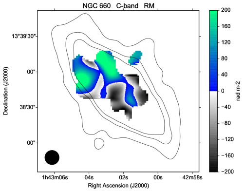
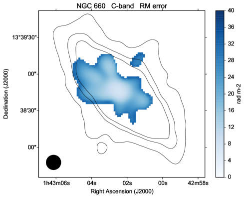
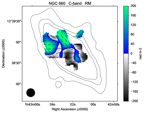
Figure 8: Polarization results for NGC 660 at C-band and $12\hbox{${}^{\prime\prime}$}$ HPBW, corresponding to $720\,\rm{pc}$. The contour levels (TP) are 70, 210, and 350 $\mu$Jy/beam. The image of the TP map is cut at 10000 $\mu$Jy/beam in order to present the disk emission well. The six panels show total intensity (TP, Stokes I) with contours at 5, 15, 25 $\sigma$ r.m.s. and intrinsic polarization vectors (upper left, panel 1), polarized intensity (PI) with intrinsic polarization vectors and the contours of TP as given in panel 1 (upper right, panel 2), percentage polarization (referred to as Perc) with TP contours of panel 1 (mid left, panel 3), rotation measure (RM) with TP contours of panel 1 (mid right, panel 4), errors in RM with TP contours of panel 1 (lower left, panel 5), rotation measure with intrinsic polarization vectors and TP contours of panel 1 (lower right, panel 6).

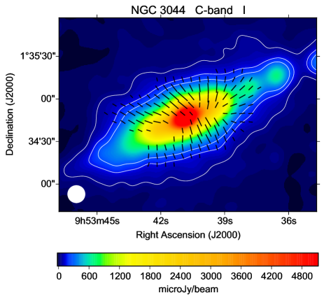
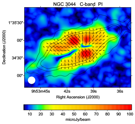
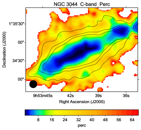
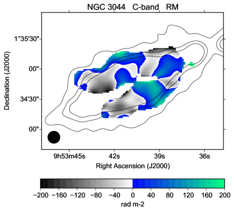
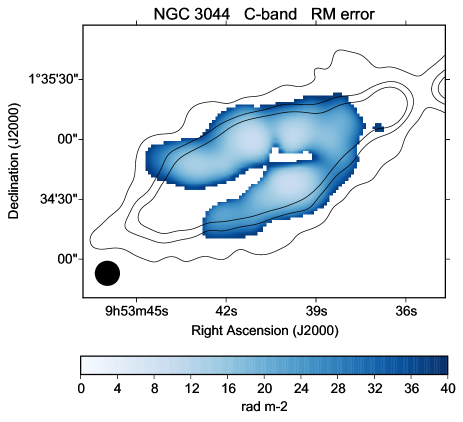
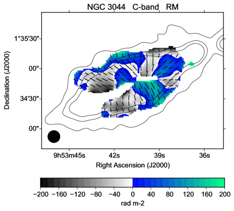
Figure 12: Polarization results for NGC 3044 at C-band and $12\hbox{${}^{\prime\prime}$}$ HPBW, corresponding to $1180\,\rm{pc}$. The contour levels (TP) are 50, 150, and 250 $\mu$Jy/beam.

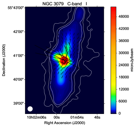
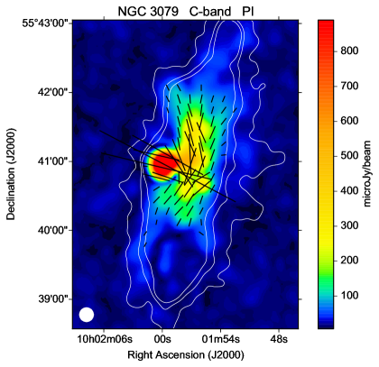
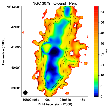
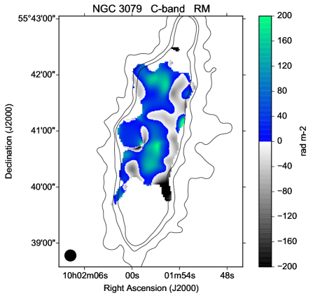
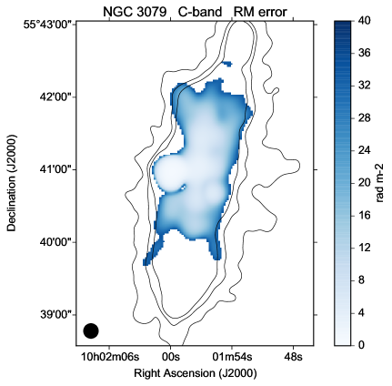
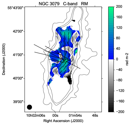
Figure 13: Polarization results for NGC 3079 at C-band and $12\hbox{${}^{\prime\prime}$}$ HPBW, corresponding to $1200\,\rm{pc}$. The contour levels (TP) are 40, 120, and 200 $\mu$Jy/beam. The image of the TP map is cut at 10000 $\mu$Jy/beam in order to present the disk emission well.

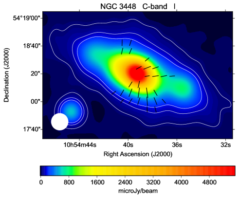
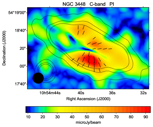
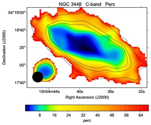
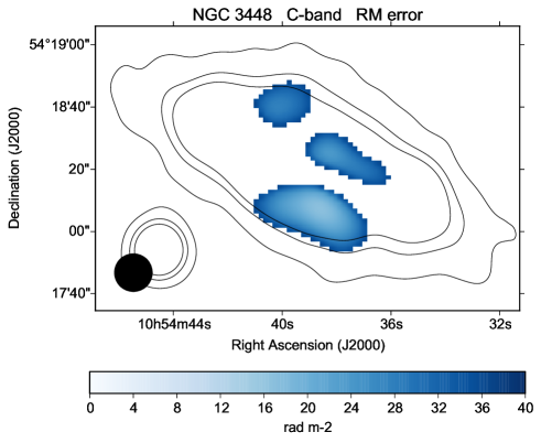
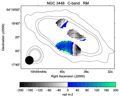
Figure 14: Polarization results for NGC 3448 at C-band and $12\hbox{${}^{\prime\prime}$}$ HPBW, corresponding to $1430\,\rm{pc}$. The contour levels (TP) are 35, 105, and 175 $\mu$Jy/beam.

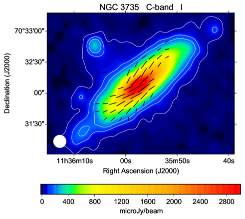
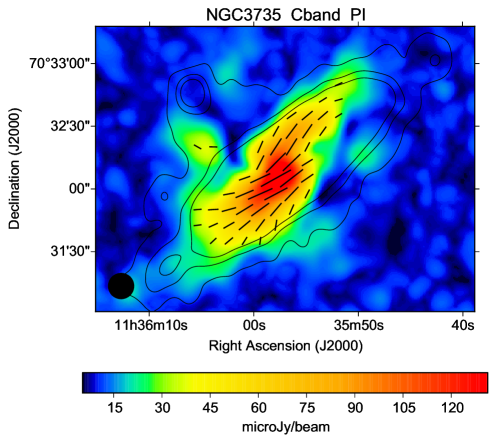
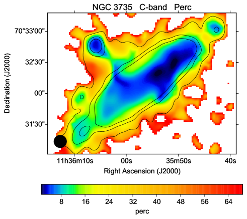
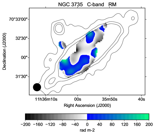
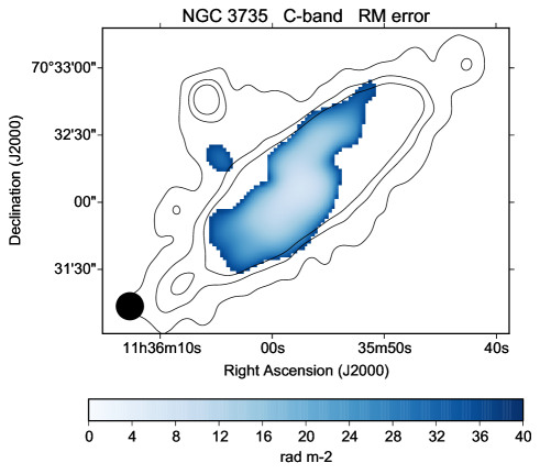
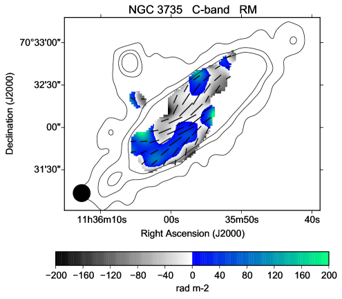
Figure 17: Polarization results for NGC 3735 at C-band and $12\hbox{${}^{\prime\prime}$}$ HPBW, corresponding to $2440\,\rm{pc}$. The contour levels (TP) are 35, 105, and 175 $\mu$Jy/beam.

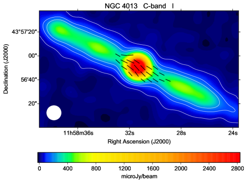
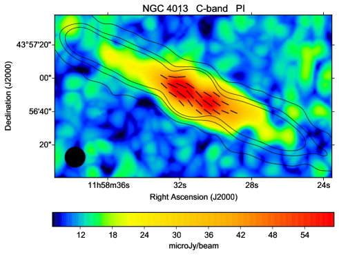
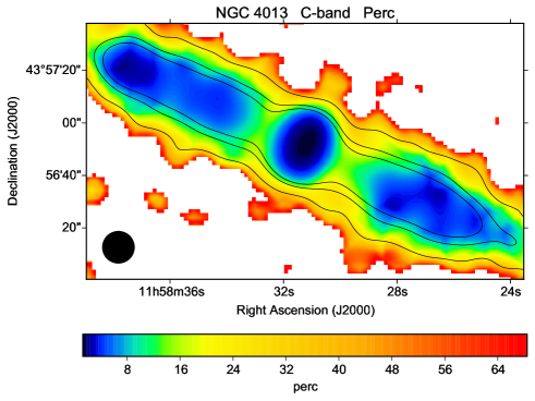
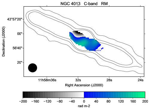
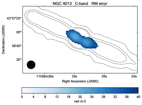
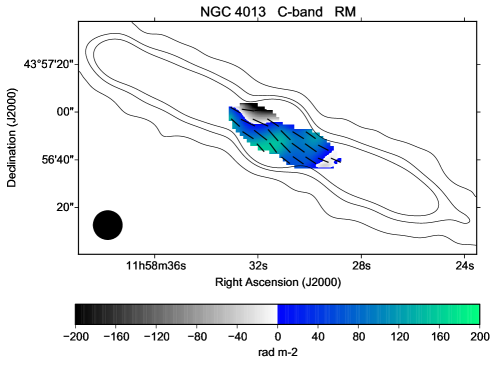
Figure 18: Polarization results for NGC 4013 at C-band and $12\hbox{${}^{\prime\prime}$}$ HPBW, corresponding to $930\,\rm{pc}$. The contour levels (TP) are 40, 120, and 200 $\mu$Jy/beam.

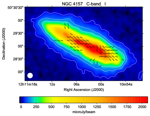
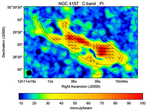
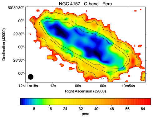
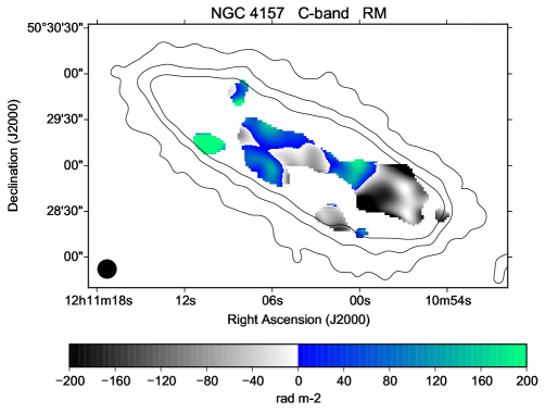
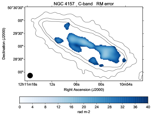
Figure 19: Polarization results for NGC 4157 at C-band and $12\hbox{${}^{\prime\prime}$}$ HPBW, corresponding to $910\,\rm{pc}$. The contour levels (TP) are 40, 120, and 200 $\mu$Jy/beam.

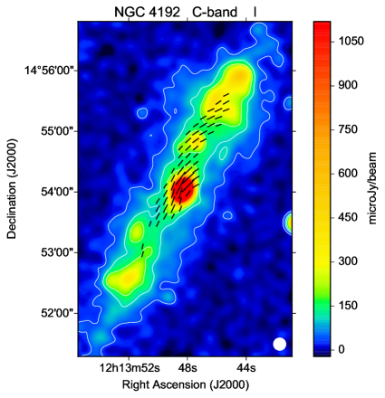
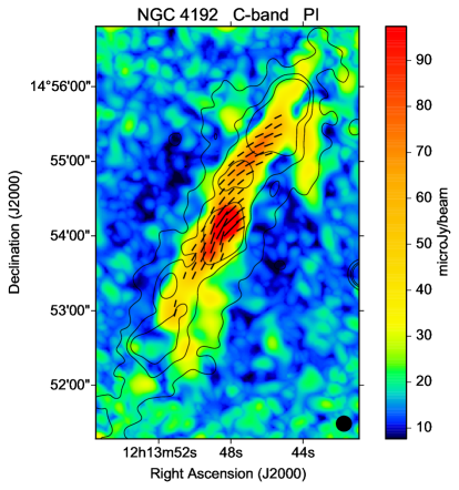
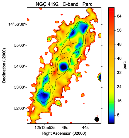
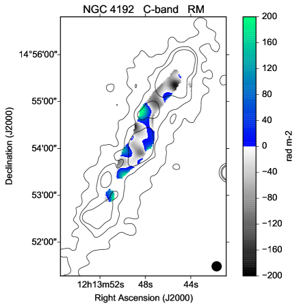
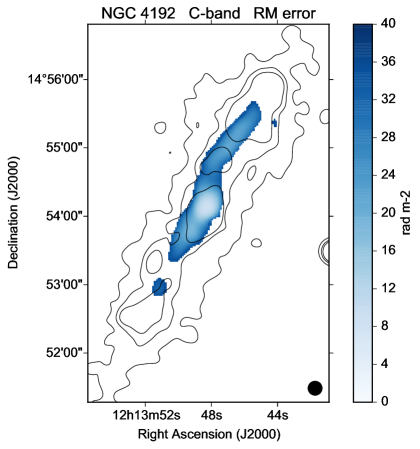
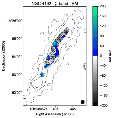
Figure 20: Polarization results for NGC 4192 at C-band and $12\hbox{${}^{\prime\prime}$}$ HPBW, corresponding to $790\,\rm{pc}$. The contour levels (TP) are 35, 105, and 175 $\mu$Jy/beam.

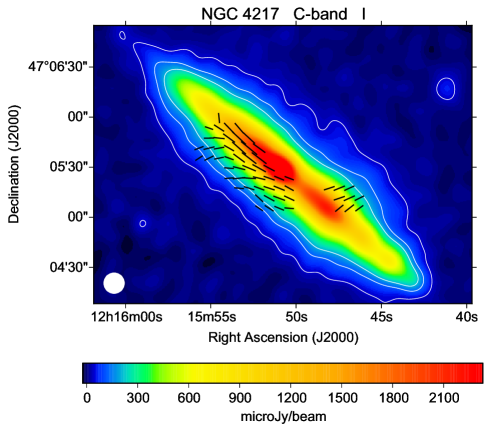
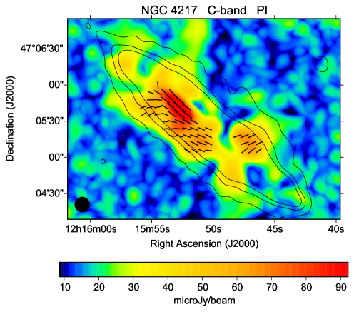
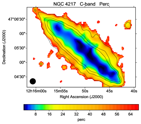
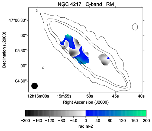
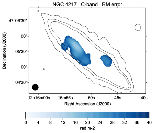
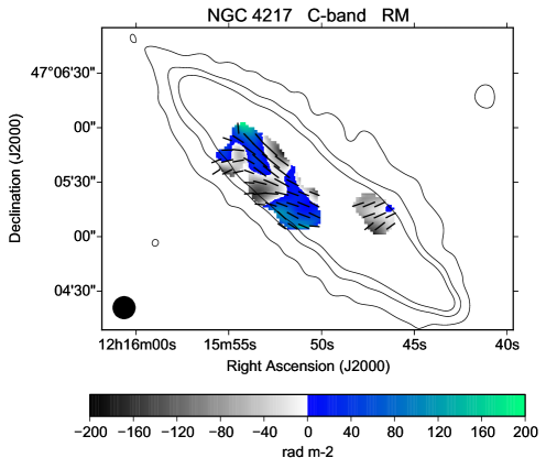
Figure 21: Polarization results for NGC 4217 at C-band and $12\hbox{${}^{\prime\prime}$}$ HPBW, corresponding to $1200\,\rm{pc}$. The contour levels (TP) are 40, 120, and 200 $\mu$Jy/beam.

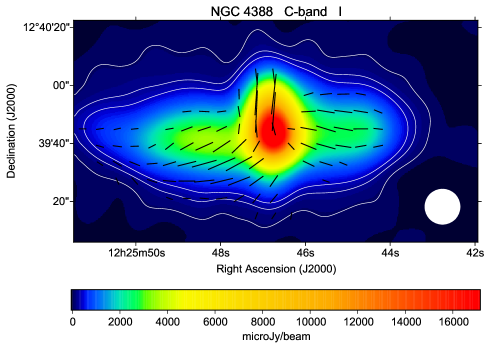
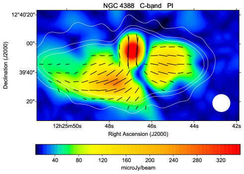
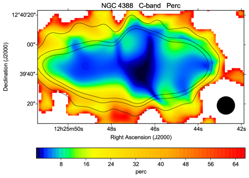
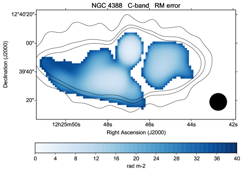
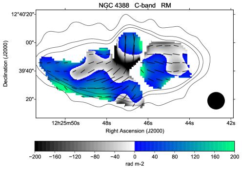
Figure 23: Polarization results for NGC 4388 at C-band and $12\hbox{${}^{\prime\prime}$}$ HPBW, corresponding to $970\,\rm{pc}$. The contour levels (TP) are 75, 225, and 375 $\mu$Jy/beam.

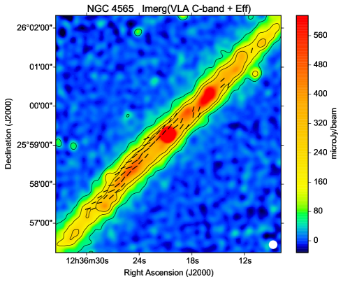
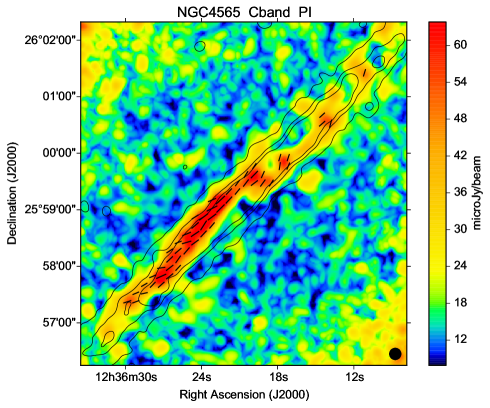
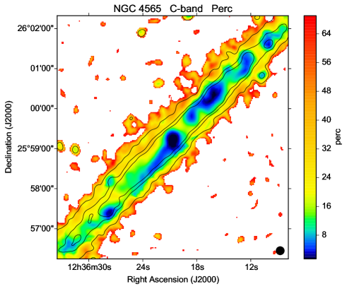
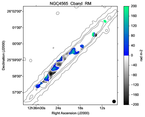
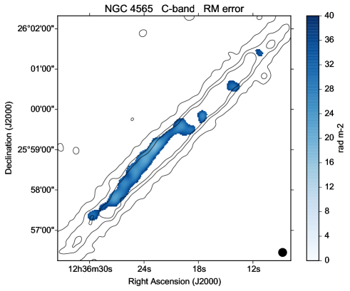
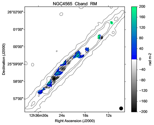
Figure 24: Polarization results for NGC 4565 at C-band and $12\hbox{${}^{\prime\prime}$}$ HPBW, corresponding to $690\,\rm{pc}$. The contour levels (TP) are 50, 150, and 250 $\mu$Jy/beam.

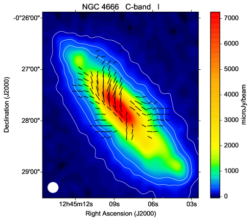
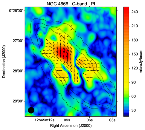
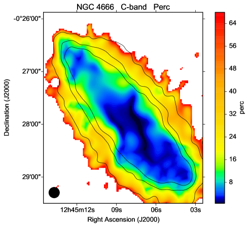
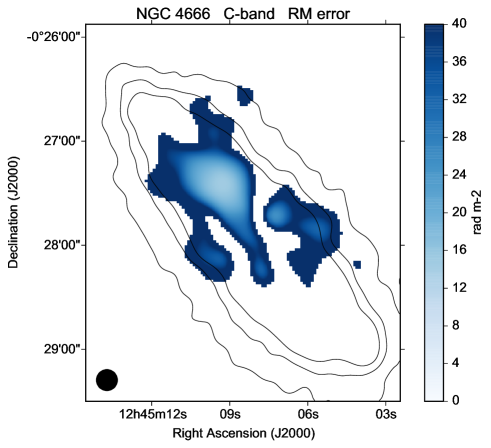
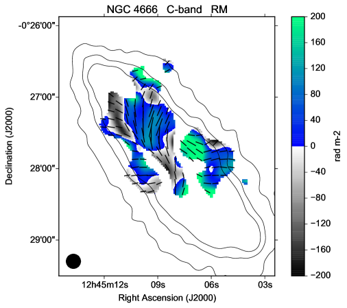
Figure 26: Polarization results for NGC 4666 at C-band and $12\hbox{${}^{\prime\prime}$}$ HPBW, corresponding to $1600\,\rm{pc}$. The contour levels (TP) are 90, 270, and 450 $\mu$Jy/beam.

Appendix B HI observation of NGC 3735

NGC 3735 was observed by the VLA under project code AC168 on 1987 March 8. The array was in D configuration, and the correlator was set up to deliver 31 channels over a 3 MHz bandwidth centred at 1407.75 MHz, in a single parallel-hand polarization (RR). The channel width corresponds to a velocity resolution of about $21\leavevmode\nobreak\ \mathrm{km\,s^{-1}}$. The total time on the target source was 57 minutes.

We used CASA version 5.4.1-31 to calibrate and image the data. Based on visual inspection of the visibilities, no flagging was required. The fluxscale was set based on the calibrator source 1634+628. Bandpass, delays, and gain phase and amplitude corrections were determined using the calibrator source 1203+645. Self-calibration was not implemented. An H i image cube was produced using task tclean, with Briggs weighting (robust=0) and no deconvolution. Continuum subtraction was carried out in the image plane. An image of the velocity at the peak of the line spectrum in each pixel was produced using the miriad task moment with mom=-3. On this basis, we determined the approaching side of the galaxy to correspond to the SE side.