The entry and exit game in the electricity markets: a mean-field game approach

Abstract

We develop a model for the industry dynamics in the electricity market, based on mean-field games of optimal stopping. In our model, there are two types of agents: the renewable producers and the conventional producers. The renewable producers choose the optimal moment to build new renewable plants, and the conventional producers choose the optimal moment to exit the market. The agents interact through the market price, determined by matching the aggregate supply of the two types of producers with an exogenous demand function. Using a relaxed formulation of optimal stopping mean-field games, we prove the existence of a Nash equilibrium and the uniqueness of the equilibrium price process. An empirical example, inspired by the UK electricity market is presented. The example shows that while renewable subsidies clearly lead to higher renewable penetration, this may entail a cost to the consumer in terms of higher peakload prices. In order to avoid rising prices, the renewable subsidies must be combined with mechanisms ensuring that sufficient conventional capacity remains in place to meet the energy demand during peak periods.

Key words: mean-field games, optimal stopping, renewable energy, electricity markets.
AMS subject classifications: 91A55, 91A13, 91A80

1 Introduction

The world electricity sector is undergoing a major transition. The large-scale deployment of renewable energy fueled by tax rebates, subsidies, and feed-in tariffs in the last 20 years has profoundly changed the market landscape: instead of large integrated utilities, a considerable fraction of electricity is now generated by small and medium-sized renewable producers. Renewable generation is already affecting prices in many countries, and its role is bound to increase. According to Internatonal Energy Agency [20], to limit the global temperature increase to 1.75^∘C by 2100 (Paris Agreement range midpoint), the energy sector must reach carbon neutrality by 2060. This objective is achievable only through massive deployment of renewable electricity. Such levels of renewable penetration may not be compatible with the present structure of electricity markets, networks and incentives. In particular, the near-zero marginal cost of electricity from renewable sources pushes down baseload wholesale electricity prices, eroding the profits of the conventional producers vital for system stability. As a result, baseload conventional producers leave the market, and the peak demand has to be met to a larger extent by peakload plants with much higher generation costs. Paradoxically, the increased renewable penetration may therefore lead to higher peak prices and increased overall electricity procurement costs [25].

The goal of this paper is to develop a game theoretical model to understand the dynamics of electricity markets under large scale renewable penetration. More precisely, we use the setting of mean-field games (MFG) to describe the evolution of the future electricity markets under different incentive schemes, to understand the effect of these policy decisions on the entry and exit of the market players and the evolution of renewable penetration and electricity prices.

We consider a stylized model with two classes of agents: (i) The intermittent (wind) producers, who generate electricity with a stochastic capacity factor at zero marginal cost. The renewable producers aim to determine the optimal moment to enter the market, by paying a sunk cost. (ii) The conventional (gas) producers with a fixed capacity, but a random running cost (depending in particular on the fuel cost and the CO2 emission cost). They aim to determine the optimal moment to exit the market. The two types of agents interact through the market price, which is deduced from the total renewable production and the total conventional capacity through a merit order mechanism, using an exogeneously specified deterministic demand function.

The theory of relaxed solutions of optimal stopping MFG, developped in [9], is used to determine the dynamic equilibrium trajectory for the baseload and peakload prices and for the conventional and renewable installed capacity. We prove the existence of a Nash equilibrium and the uniqueness of the equilibrium price process. Our proofs are based on technical tools specific to this particular problem, which are not entirely covered by [9]: in particular, the price functional deduced from the merit order mechanism is highly irregular and requires special treatment.

A numerical illustration, inspired by the UK electricity market is presented, and allows to conclude that while renewable subsidies clearly lead to higher renewable penetration, this may entail a cost to the consumer in terms of higher peakload prices. In order to avoid rising prices, the renewable subsidies must be combined with market or off-market mechanisms ensuring that sufficient conventional capacity remains in place to meet the energy demand during peak periods.

The paper is structured as follows. In the remaining part of the introduction we review the relevant literautre. Section 2 presents our model of the electricity market. The relaxed solution approach and the main theoretical results are exposed in Section 3. The numerical computation of the MFG solution is presented in Section 4 and a concrete example is discussed in Section 5. Finally, in Appendix, we provide the detailed proof of a technical result used in the paper.

Literature review

Several papers consider the effect of increased renewable penetration on market prices of electricity both in the long-term [11] and short-term [22] setting. Recent papers also study the interactions between energy and capacity markets in the presence of market power, that is, the ability of producers to willingly influence prices in a way favorable for them, and the role of renewables in such interactions. Schwenen [28] provides empirical evidence of market power in the New York capacity market. Fabra [14] uses a microeconomic model to study the effects of market power in the capacity market on the performance of energy markets. Benatia [6] studies strategic bidding in New York’s energy market.

Many authors have analyzed possible market evolutions and alternative designs to ensure system reliability and economic viability. Henriot and Glachant [19] discuss alternative schemes for market integration of renewable generators, Levin and Botterud [24] analyze and compare different market designs to ensure generator revenue sufficiency and Rious et al. [27] study the market design to encourage the development of demand response and improve system flexibility. A particularly important innovation has been the introduction of capacity markets, surveyed in [10]. The above papers mainly analyze the structure of existing markets and make proposals for improvement but do not use models to simulate the evolution of future markets under alternative design proposals. This line of research has been pursued by by some authors using computational agent-based modeling (see e.g. [8] for an application to the capacity market).

The game theory has been applied to the modeling of entry/exit decisions of agents in electricity markets in [29], where a system of two producers is considered, and the price is not affected by the agents’ decisions. A considerable literature is devoted to capacity expansion games in energy markets, see e.g., [1]. A related strand of literature uses computational agent-based models to understand the dynamics of wholesale electricity markets, see [31] for a review. These models allow for heterogeneous agents and a precise description of the market structure, but are computationally very intensive and do not provide any insight about the model (uniqueness of the equilibrium, robustness etc.) beyond what can be recovered from a simulated trajectory.

The machinery of MFG appears to be a promising compromise between the complexity of computational agent-based models and the tractability of fully analytic approaches. MFG, introduced in [23] are stochastic games with a large number of identical agents and symmetric interactions where each agent interacts with the average density of the other agents (the mean field) rather than with each individual agent. This simplifies the problem, leading to explicit solutions or efficient numerical methods for computing the equilibrium dynamics. In the recent years MFG have been successfully used to model specific sectors of electricity markets, such as price formation [17], electric vehicles [12], demand dispatch [4] and storage [2]. An important recent development is the introduction of MFG of optimal stopping / obstacle mean-field games [7, 9, 15], which can describe technology switches and entry/exit decisions of players. In this paper, we follow the relaxed solution approach of [9] (see also [16] for a related notion of relaxed solution), and extend the theoretical results of that paper to allow for two classes of agents and enable the agents to interact through the market price, which is an irregular functional not covered by the assumptions in [9].

2 The model

We fix a terminal time horizon $T$ and consider a model of electricity market with exogeneous demand and producing agents of two different types. In this section, we describe the model for a finite number of agents, before passing to the MFG limit in the following ones.

Conventional producers

The maximum capacity of all conventional producers is assumed to be identical and fixed; the plants can operate at zero, full or partial capacity. Each conventional producer has a marginal cost function

$$C^{i}_{t}:[0,1]\mapsto\mathbb{R},$$

in other words, if the plant is operating at a fraction $\xi$ of its total capacity, $C^{i}_{t}(\xi)$ corresponds to the unit cost of producing an additional infinitesimal amount of energy. We assume that

$$C^{i}_{t}(\xi)=C^{i}_{t}+c(\xi),$$

where $C^{i}_{t}$ is the baseline cost process and $c:\mathbb{R}_{+}\mapsto[0,1]$ is a deterministic strictly increasing smooth function with $c(0)=0$. This increasing property is justified by the need to start up additional less efficient units, recall additional employees etc. Consequently, for a given price level $p$, the producer offers a fraction $F(p-C^{i}_{t})$ of its total capacity, where $F$ is the inverse mapping of $c$. $F$ is also a smooth increasing function, and it satisfies $F(y)=0$ for $y\leq 0$, $F(y)>0$ for $y>0$ and $F(y)=1$ for $y\geq c(1)$. In other words, the producer does not offer any capacity if the price is less than the production cost, and as the price increases beyond the production cost, the producer gradually offers more capacity, until reaching the full capacity at a sufficiently high price level.

The baseline cost is assumed to follow the CIR process:

$$dC^{i}_{t}=k(\theta-C^{i}_{t})dt+\delta\sqrt{C^{i}_{t}}dW^{i}_{t},\quad C^{i}_{0}=c_{i},$$ (1)

where $(W^{i})_{i\geq 1}$ are independent standard Brownian motions, $\theta$ is the long-term average cost, $k$ is the rate of mean reversion and $\delta$ determines the variability of the cost process. The conventional producers aim to exit the market at the optimal time $\tau_{i}$. We denote by $\omega^{n}_{t}(dx)$ the distribution of costs of conventional producers who have not yet exited the market (when there are a total of $n$ producers in the beginning of the game). In other words,

$$\omega^{n}_{t}(dx)=\frac{1}{n}\sum_{i=1}^{n}\delta_{C^{i}_{t}}(dx)\mathbf{1}_{\tau_{i}>t}.$$

Note that we have normalized the distribution by the number of producers, which turns out to be convenient at a later stage. This is equivalent to assuming that the capacity of each producer equals $\frac{1}{n}$.

Renewable producers

Renewable producers aim to enter the market at the optimal time $\sigma_{i}$. To enter the market (build the power plant) they pay the cost $K_{R}$ after which the plant generates $S^{i}_{t}\in(0,1)$ units of electricity per unit time at zero cost, where the intermittent output $S^{i}$ follows the Jacobi process

$$dS^{i}_{t}=\bar{k}(\bar{\theta}-S^{i}_{t})dt+\bar{\delta}\sqrt{S^{i}_{t}(1-S^{i}_{t})}d\overline{W}^{i}_{t},\quad S^{i}_{0}=s_{i}\in(0,1),$$ (2)

where $(\overline{W}_{i})_{i\geq 1}$ are standard Brownian motions, independent from each other and from the price processes of conventional producers. With this model we are not attempting to describe the high-frequency variation of the power output due to the intermittency of the renewable resource, but rather the slow variation of the capacity factor due to climate variability and other effects.

We assume that there are $n$ potential renewable projects in the beginning of the game, which may enter the market at some time. We denote by $\eta^{n}_{t}(dx)$ the (potential) distribution of output of renewable producers who have not yet entered the market:

$$\eta_{t}(dx)=\frac{1}{n}\sum_{i=1}^{n}\delta_{S^{i}_{t}}(dx)\mathbf{1}_{\sigma_{i}>t}.$$

We shall also need the distribution of output values of all renewable projects:

$$\bar{\eta}^{n}_{t}(dx)=\frac{1}{n}\sum_{i=1}^{n}\delta_{S^{i}_{t}}(dx).$$

Note that both distributions are also normalized by the number of agents. The normalization allows to simplify some expressions but our model can easily be extended to the case when the number of conventional producers is different from that of the renewable projects, or when the capacities of these two types of agents are different.

We denote by $\mathcal{L}$ the infinitesimal generator of the process $C^{i}$ and by $\overline{\mathcal{L}}$ that of $S^{i}$. These are given by

$$\mathcal{L}f =k(\theta-x)\frac{\partial f}{\partial x}+\frac{\delta^{2}x}{2}\frac{\partial^{2}f}{\partial x^{2}},$$

$$\overline{\mathcal{L}}f =\bar{k}(\bar{\theta}-x)\frac{\partial f}{\partial x}+\frac{\bar{\delta}^{2}x(1-x)}{2}\frac{\partial^{2}f}{\partial x^{2}}.$$

The state spaces are denoted by $\Omega$ and $\overline{\Omega}$, respectively.

Gain function of conventional producers

At time $t$ and price level $p$, each conventional producer solves the profit maximisation problem

$$\max_{\xi}p\xi-\int_{0}^{\xi}C^{i}_{t}(\xi)d\xi.$$

The optimal fraction is $\xi^{\ast}:=c^{-1}(p-C^{i}_{t})$ if $p\geq C^{i}_{t}$. Thus, the profit of the producer is

$$p\xi^{\ast}-\int_{0}^{\xi^{\ast}}C^{i}_{t}(\xi)d\xi=(p-C^{i}_{t})F(p-C^{i}_{t})-\int_{0}^{F(p-C^{i}_{t})}c(\xi)d\xi:=G(p-C^{i}_{t}),$$

where

$$G(x) =xF(x)-\int_{0}^{F(x)}c(\xi)d\xi=\int_{0}^{F(x)}(x-c(\xi))d\xi=\int_{0}^{x}F(z)dz,$$

where the second equality results from a change of variable using the fact that $F$ is the inverse of $c$.

The problem of the individual conventional producer is then

$${\max_{\tau\in\mathcal{T}([0,T])}\mathbb{E}\left[\int_{0}^{\tau}e^{-\rho t}(G(P^{n}_{t}-C^{i}_{t})-\kappa_{C})dt+K_{C}e^{-(\gamma_{C}+\rho)\tau}\right],}$$

where $\mathcal{T}([0,T])$ represents the set of stopping times with respect to the filtration generated by $(W_{t}^{i})_{i\geq 1}$,$(\bar{W}^{i})_{i\geq 1}$, with values between $0$ and $T$. Here $P^{n}_{t}$ is the market price of electricity, determined from the strategies of all agents via the merit order mechanism described below in this section, $\kappa_{C}$ is the fixed cost per unit of time that the producer pays until exiting the market and $e^{-\gamma_{C}t}K_{C}$ is the value recovered if the plant is sold at time $t$, where $\gamma_{C}$ is the depreciation rate of the conventional plant. To avoid a discontinuity at the terminal date $T$, we assume that the plant is sold at date $T$ in any case. This maximization problem may equivalently be written as

$${\max_{\tau\in\mathcal{T}([0,T])}}\mathbb{E}\left[\int_{0}^{T}e^{-\rho t}\mathbf{1}_{t<\tau}\left\{G(P^{n}_{t}-C^{i}_{t})-\kappa_{C}-e^{-\gamma_{C}t}K_{C}(\rho+\gamma_{C})\right\}dt\right],$$

or, with a more compact notation,

$${\max_{\tau\in\mathcal{T}([0,T])}}\mathbb{E}\left[\int_{0}^{T}e^{-\rho t}\mathbf{1}_{t<\tau}\left\{G(P^{n}_{t}-C^{i}_{t})+f_{C}(t)\right\}dt\right],$$

$$f_{C}(t)=-\kappa_{C}-e^{-\gamma_{C}t}K_{C}(\rho+\gamma_{C}).$$

Gain function of renewable producers

The renewable producers always bid their full (but intermittent) capacity. We assume that the prices are always positive, and neglect the forecasting error of the producers. The problem of the individual agent is then

$${\max_{\sigma\in\mathcal{T}([0,T])}\mathbb{E}\left[\int_{\sigma}^{T}e^{-\rho t}(P^{n}_{t}S^{i}_{t}-\kappa_{R})dt-K_{R}e^{-\rho\sigma}+K_{R}e^{-\rho T-\gamma_{R}(T-\sigma)}\right],}$$

where $\sigma$ is the time of entering the market, $\kappa_{R}$ is the fixed cost of owning the plant, $K_{R}$ is the fixed cost of building the plant and $K_{R}^{-\gamma_{R}(T-\sigma)}$ is the value of the plant at time $T$, where $\gamma_{R}$ is the depreciation rate of the renewable plant. Once again, to minimize the boundary effect, we assume that the agent recovers the value of the plant reduced by the depreciation rate at the terminal date $T$. This maximization problem may equivalently be written as

$$\max_{\sigma\in\mathcal{T}([0,T])}\mathbb{E}\left[\int_{0}^{T}\mathbf{1}_{t<\sigma}e^{-\rho t}\left\{-P^{n}_{t}S^{i}_{t}+\kappa_{R}+\rho K_{R}+\gamma_{R}K_{R}e^{-(\rho+\gamma_{R})(T-t)}\right\}\right],$$

or, with a more compact notation,

$$\max_{\sigma\in\mathcal{T}([0,T])}\mathbb{E}\left[\int_{0}^{T}\mathbf{1}_{t<\sigma}e^{-\rho t}\left\{-P^{n}_{t}S^{i}_{t}+f_{R}(t)\right\}\right],$$

$$f_{R}(t)=\kappa_{R}+\rho K_{R}+\gamma_{R}K_{R}e^{-(\rho+\gamma_{R})(T-t)}.$$

Baseline supply

We assume that in addition to the renewable and conventional producers considered above there is a baseline supply by conventional producers, which will never leave the market (e.g., state-owned producers, which ensure the network security) and do not take part in the game. This baseline supply at price level $p$ is denoted by $F_{0}(p)$ where the function $F_{0}$ is increasing and satisfies $F_{0}(0)=0$, $F_{0}(p+h)-F(p)\geq ch$ for some $c>0$ and all $p,h\geq 0$. This last assumption is imposed for techical reasons and ensures the continuity of the equilibrium price process.

The total supply by the conventional producers at price level $p$, including the baseline supply, is therefore given by

$$\int_{\Omega}F(p-x)\omega^{n}_{t}(dx)+F_{0}(p).$$

The total renewable supply at time $t$, on the other hand, is given by

$${R^{n}_{t}=\int_{\overline{\Omega}}x(\bar{\eta}^{n}_{t}(dx)-\eta^{n}_{t}(dx))}.$$

Price formation

In our model, the different agents are coupled through the market price, determined by matching the exogeneous demand process $\overline{D}_{t}$, to the aggregate supply function of market participants, in a stylized version of the day-ahead electricity market. In other words, since the residual demand after subtracting the renewable supply which is always present in the market, must be met by conventional producers, the electricity price $P^{n}_{t}$ is defined as follows.

$$P^{n}_{t}=\inf\{P:(\overline{D}_{t}-R^{n}_{t})^{+}\leq\int_{\Omega}F(P-x)\omega^{n}_{t}(dx)+F_{0}(P)\}\wedge\overline{P},$$

where $\overline{P}$ is the price cap in the market and we use the convention $\inf\emptyset=+\infty$. When the price cap $\overline{P}$ is reached, the demand may not be entirely satisfied by the producers.

Our aim here is not to model the daily price fluctuations but rather the slow evolution of the average market price due to changes of structure of electricity supply. However, to make the illustration more realistic, in section 5 we shall consider separately the peak price (Mon-Fri, 7AM-8PM) and the off-peak price. This extension presents no technical difficulties, and therefore, to simplify notation, we consider a single price in the rest of the paper.

3 Relaxed MFG formulation of the problem

To simplify the resolution and the study of price equilibria, we place ourselves from now on in the MFG framework, where the number of agents (both conventional and renewable) is assumed to be infinite. As in many papers on mean-field games, we do not study the convergence of the $n$-player game to the MFG but analyze the MFG framework directly. We denote the limiting versions of the distributions $\omega^{n}_{t}$, $\eta^{n}_{t}$ and $\bar{\eta}^{n}_{t}$ by $\omega_{t}$, $\eta_{t}$ and $\bar{\eta}_{t}$, respectively, and the limiting market price and renewable demand by $P_{t}$ and $R_{t}$. Since in our game the idiosyncratic noises of agents are independent and there is no common noise, these limiting measures and processes are assumed to be deterministic. Note that $\omega_{t}$ and $\eta_{t}$ are not probability distributions: the total mass of both these measures is decreasing with $t$. We finally assume that the demand $\overline{D}_{t}$ is deterministic.

We follow the relaxed optimal stopping MFG approach, introduced in [9], adapting it to the present setting of electricity markets. To this end, we first recall the topology on flows of measures used in this reference. Let $V_{\Omega}$ be the space of flows of signed bounded measures on ${\Omega}$, $(m_{t}(\cdot))_{0\leq t\leq T}$ such that: for every $t\in[0,T]$, $m_{t}$ is a signed bounded measure on ${\Omega}$, for every $A\in\mathcal{B}({\Omega})$, the mapping $t\mapsto m_{t}(A)$ is measurable, and $\int_{0}^{T}\int_{{\Omega}}m_{t}(dx)\,dt<\infty$. To each flow $m\in V_{\Omega}$, we associate a signed measure on $[0,T]\times{\Omega}$ defined by $\mu(dt,dx):=m_{t}(dx)\,dt$, and we endow $V_{\Omega}$ with the topology of weak convergence of the associated measures. $V_{\overline{\Omega}}$ is defined in the same way.

Given a deterministic measurable price process $(P_{t})_{t\geq 0}$, the relaxed solution approach consists in replacing the optimal stopping problem of individual conventional producer,

$$\sup_{\tau}\mathbb{E}\left[\int_{0}^{T}e^{-\rho t}[G(P_{t}-C_{t})+f_{C}(t)]\mathbf{1}_{t<\tau}dt\right],$$ (3)

by its relaxed version

$$\sup_{\omega\in\mathcal{A}(\omega_{0})}\int_{0}^{T}\int_{\Omega}e^{-\rho t}[G(P_{t}-x)+f_{C}(t)]\omega_{t}(dx)\,dt,$$ (4)

where the set $\mathcal{A}(\omega_{0})$ contains all flows of positive bounded measures $(\hat{\omega}_{t})_{0\leq t\leq T}\in V_{\Omega}$ satisfying

$$\int_{\Omega}u(0,x)\omega_{0}(dx)+\int_{0}^{T}\int_{\Omega}\left\{\frac{\partial u}{\partial t}+\mathcal{L}u\right\}\hat{\omega}_{t}(dx)\,dt\geq 0$$

for all $u\geq 0,u\in C^{1,2}([0,T]\times\Omega)$ such that $\frac{\partial u}{\partial t}+\mathcal{L}u$ is bounded.

In the relaxed formulation of the optimal stopping problem, instead of looking for an optimal stopping time, one looks for the optimal measure flow, corresponding, at each time $t$, to the distribution of agents in a population which have not yet exited the game. The precise relationship between the optimal stopping problem (3) and its relaxed version (4) is described in [9]. In particular, under appropriate assumptions, it holds that

$$\sup_{\omega\in\mathcal{A}(\omega_{0})}\int_{0}^{T}\int_{\Omega}e^{-\rho t}[G(P_{t}-x)+f_{C}(t)]\omega_{t}(dx)\,dt=\int_{\Omega}v(0,x)\omega_{0}(dx),$$

where $v(0,x)$ is the value function of the optimal stopping problem (3) at time $t=0$:

$$v(0,x)=\sup_{\tau}\mathbb{E}\left[\int_{0}^{T}e^{-\rho t}[G(P_{t}-C^{(0,x)}_{t})+f_{C}(t)]\mathbf{1}_{t<\tau}dt\right]$$

Similarly, the optimal stopping problem of individual renewable producer

$$\sup_{\sigma}\mathbb{E}\left[\int_{0}^{T}e^{-\rho t}\left\{-P_{t}S_{t}+f_{R}(t)\right\}\mathbf{1}_{t<\sigma}dt\right]$$

is replaced by its relaxed version

$$\sup_{\eta\in\overline{\mathcal{A}}(\eta_{0})}\int_{0}^{T}\int_{\overline{\Omega}}e^{-\rho t}\left\{-P_{t}x+f_{R}(t)\right\}\eta_{t}(dx)\,dt,$$ (5)

where the set $\overline{\mathcal{A}}(\eta_{0})\subset V_{\overline{\Omega}}$ is defined similarly to ${\mathcal{A}}(\omega_{0}).$

Given the flows $(\omega_{t})_{0\leq t\leq T}$ and $(\eta_{t})_{0\leq t\leq T}$, the price process $(P_{t})_{0\leq t\leq T}$ is defined as follows.

$$P_{t}=\inf\{P:(\overline{D}_{t}-R_{t})^{+}\leq\int_{\Omega}F(P_{t}-x)\omega_{t}(dx)+F_{0}(P_{t})\}\wedge\overline{P},\quad 0\leq t\leq T,$$

where ${R_{t}=\int_{\overline{\Omega}}x(\bar{\eta}_{t}(dx)-\eta_{t}(dx))}$. We denote the price, defined in this way, by $P_{t}(\omega_{t},\eta_{t})$.

We now introduce the definition of a relaxed Nash equilibrium.

Definition 1.

The Nash equilibrium of the relaxed mean-field game is the couple $(\omega^{*}_{t},\eta^{*}_{t})$ such that for any other measure $\omega\in\mathcal{A}(\omega_{0})$,

$$\int_{0}^{T}\int_{\Omega}e^{-\rho t}[G(P_{t}(\omega^{*}_{t},\eta^{*}_{t})-x)+f_{C}(t)]\omega_{t}(dx)\,dt\\ \leq\int_{0}^{T}\int_{\Omega}e^{-\rho t}[G(P_{t}(\omega^{*}_{t},\eta^{*}_{t})-x)+f_{C}(t)]\omega^{*}_{t}(dx)\,dt,$$

and for any other measure $\eta\in\overline{\mathcal{A}}(\eta_{0})$

$$\int_{0}^{T}\int_{\overline{\Omega}}e^{-\rho t}[-P_{t}(\omega^{*}_{t},\eta^{*}_{t})x+f_{R}(t)]\eta_{t}(dx)\,dt\\ \leq\int_{0}^{T}\int_{\overline{\Omega}}e^{-\rho t}[-P_{t}(\omega^{*}_{t},\eta^{*}_{t})x+f_{R}(t)]\eta^{*}_{t}(dx)\,dt.$$

In the rest of this section we study the solutions of the relaxed MFG problem. Firsly, the following lemma establishes the existence of solution for the individual relaxed optimal stopping problems.

Lemma 1.

Let the price process $(P_{t})_{0\leq t\leq T}$ be fixed, and asume that it has bounded variation on $[0,T]$.

• Let $\omega_{0}$ satisfy

  $$\int_{\Omega}\ln\{1+|x|\}\omega_{0}(dx)<\infty.$$

  Then there exists $\omega^{*}\in\mathcal{A}(\omega_{0})$ which solves the problem (4).

• Let $\eta_{0}$ satisfy

  $$\int_{\overline{\Omega}}\ln\{1+|x|\}\eta_{0}(dx)<\infty.$$

  Then there exists $\eta^{*}\in\overline{\mathcal{A}}(\eta_{0})$ which solves the problem (5).

Proof.

Part i. Choose a maximizing sequence of flows of measures $(\omega^{n}_{t})_{t\in[0,T]}^{n\geq 1}\subset\mathcal{A}(\omega_{0})$. By Lemma 3.8 in [9], the set $\mathcal{A}(\omega_{0})$ is sequentially compact, therefore this sequence has a subsequence, also denoted by $(\omega^{n})$, which converges to a limit $\omega^{*}\in\mathcal{A}(m^{*}_{0})$. It remains to show that $\omega^{*}$ is a maximizer of (4). Let $(P^{m}_{t})^{m\geq 1}$ be a sequence of uniformly bounded continuous mappings approximating $P_{t}$ in $L^{1}([0,T])$. Note that $G$ is a Lipschitz function, with Lipschitz constant $1$. Then,

$$\int_{0}^{T}dt\int_{\Omega}[G(P_{t}-x)+f_{C}(t)]\omega^{n}_{t}(dx) =\int_{0}^{T}dt\int_{\Omega}[G(P^{m}_{t}-x)+f_{C}(t)]\omega^{n}_{t}(dx)$$

$$+\int_{0}^{T}dt\int_{\Omega}[G(P_{t}-x)-G(P^{m}_{t}-x)]\omega^{n}_{t}(dx).$$ (6)

The second term satisfies

$$\left|\int_{0}^{T}dt\int_{\Omega}[G(P_{t}-x)-G(P^{m}_{t}-x)]\omega^{n}_{t}(dx)\right|\leq\int_{0}^{T}|P_{t}-P^{m}_{t}|\int_{\Omega}\omega^{n}_{t}(dx)$$ (7)

Taking the test function

$$u(t,x)=\int_{t}^{T}f(s)ds$$

with $f\geq 0$ continuous in the definition of $\mathcal{A}(\omega_{0})$, we have:

$$\int_{\Omega}\omega_{0}(dx)\int_{0}^{T}f(s)ds\geq\int_{0}^{T}f(s)ds\int_{\Omega}\omega^{n}_{t}(dx).$$

This implies that for every $n$, $t$-almost everywhere,

$$\int_{\Omega}\omega^{n}_{t}(dx)\leq\int_{\Omega}\omega_{0}(dx),$$

and so (7) converges to zero as $m\to\infty$, uniformly on $n$. On the other hand, by weak convergence, the first term in (6) converges to

$$\int_{0}^{T}dt\int_{\Omega}[G(P^{m}_{t}-x)+f_{C}(t)]\omega^{*}_{t}(dx),$$

which, once again, converges to

$$\int_{0}^{T}dt\int_{\Omega}[G(P_{t}-x)+f_{C}(t)]\omega^{*}_{t}(dx)$$

as $m\to\infty$. Combining the three limits and using the fact that the convergence of (7) is uniform on $n$, the proof is completed.

Part ii. This part is shown similarly to the first part. ∎

In the mean-field game context, the price becomes a function of $\eta_{t}$ and $\omega_{t}$. The following technical lemma establishes the properties of the price process. Its proof is presented in the appendix.

Lemma 2.

• Let $\omega\in\mathcal{A}(\omega_{0})$ and $\eta\in\overline{\mathcal{A}}(\eta_{0})$ and assume that the demand $\overline{D}$ has bounded variation on $[0,T]$. Then the price process $P_{t}(\omega_{t},\eta_{t})$ has bounded variation on $[0,T]$ as well.

• Let $(\omega^{n}_{t})$ and $(\eta^{n}_{t})$ be sequences of elements of $\mathcal{A}(\omega_{0})$ and $\overline{\mathcal{A}}(\eta_{0})$, converging, respectively, to $\omega^{*}\in\mathcal{A}(\omega_{0})$ and $\eta^{*}\in\overline{\mathcal{A}}(\eta_{0})$. Assume that the demand $\overline{D}$ has bounded variation on $[0,T]$. Then there exists a subsequence $(n_{k})_{k\geq 0}$ such that $P_{t}(\omega^{n_{k}}_{t},\eta^{n_{k}}_{t})$ converges to $P_{t}(\omega^{*}_{t},\eta^{*}_{t})$ in $L^{1}([0,T])$.

We now prove the existence of a relaxed Nash equilibrium.

Proposition 1.

There exists a Nash equilibrium for the relaxed MFG problem.

Proof.

Following the ideas of Theorem 4.4 in [9], we define the set valued mapping

$$\Theta:(\omega,\eta)\mapsto \operatorname*{arg\,max}_{\hat{\omega}\in\mathcal{A}(\omega_{0})}\int_{0}^{T}\int_{\Omega}e^{-\rho t}[G(P_{t}(\omega_{t},\eta_{t})-x)+f_{C}(t)]\hat{\omega}_{t}(dx)\,dt$$

$$\times\operatorname*{arg\,max}_{\hat{\eta}\in\overline{\mathcal{A}}(\eta_{0})}\int_{0}^{T}\int_{\overline{\Omega}}e^{-\rho t}[-P_{t}(\omega_{t},\eta_{t})x+f_{R}(t)]\hat{\eta}_{t}(dx)\,dt.$$

To establish existence of Nash equilibrium by applying Fan-Glicksberg fixed point theorem, it is enough to show that $\Theta$ has closed graph, which is defined by

$$\text{Gr}(\Theta)=\{(\omega,\bar{\omega},\eta,\bar{\eta})\in\mathcal{A}(\omega_{0})^{2}\times\overline{\mathcal{A}}(\eta_{0})^{2}:(\omega,\eta)\in\Theta(\bar{\omega},\bar{\eta})\}$$

To prove that $\text{Gr}(\Theta)$ is closed it is in turn sufficient to show that for any two sequences $(\omega^{n},\bar{\omega}^{n})_{n\geq 1}\in\mathcal{A}(\omega_{0})^{2}$, $(\eta^{n},\bar{\eta}^{n})_{n\geq 1}\in\bar{\mathcal{A}}(\eta_{0})^{2}$, which converge weakly to $(\omega,\bar{\omega})\in(\mathcal{A}(\omega_{0}))^{2}$ (resp.$(\eta,\bar{\eta})\in(\bar{\mathcal{A}}(\eta_{0}))^{2}$ ) and such that

$$\int_{0}^{T}dt\int_{\Omega}e^{-\rho t}[G(P_{t}(\omega^{n}_{t},\eta^{n}_{t})-x)+f_{C}(t)]\bar{\omega}^{n}_{t}(dx)\\ \geq\int_{0}^{T}dt\int_{\Omega}e^{-\rho t}[G(P_{t}(\omega^{n}_{t},\eta^{n}_{t})-x)+f_{C}(t)]\hat{\omega}_{t}(dx),\,\,{\rm for\,\,all\,\,}\hat{\omega}\in\mathcal{A}(\omega_{0})$$

and

$$\int_{0}^{T}\int_{\overline{\Omega}}e^{-\rho t}[-P_{t}(\omega^{n}_{t},\eta^{n}_{t})x+f_{R}(t)]\bar{\eta}^{n}_{t}(dx)\,dt\\ \geq\int_{0}^{T}dt\int_{\overline{\Omega}}e^{-\rho t}[-P_{t}(\omega^{n}_{t},\eta^{n}_{t})x+f_{R}(t)]\hat{\eta}_{t}(dx),\,\,{\rm for\,\,all\,\,}\hat{\eta}\in\bar{\mathcal{A}}(\eta_{0}),$$

we have

$$\int_{0}^{T}dt\int_{\Omega}e^{-\rho t}[G(P_{t}(\omega_{t},\eta_{t})-x)+f_{C}(t)]\bar{\omega}_{t}(dx)\\ \geq\int_{0}^{T}dt\int_{\Omega}e^{-\rho t}[(G(P_{t}(\omega_{t},\eta_{t})-x)+f_{C}(t)]\hat{\omega}_{t}(dx),\,\,{\rm for\,\,all\,\,}\hat{\omega}\in\mathcal{A}(\omega_{0})$$

and

$$\int_{0}^{T}\int_{\overline{\Omega}}e^{-\rho t}[-P_{t}(\omega_{t},\eta_{t})x+f_{R}(t)]\bar{\eta}_{t}(dx)\,dt\\ \geq\int_{0}^{T}dt\int_{\overline{\Omega}}e^{-\rho t}[-P_{t}(\omega_{t},\eta_{t})x+f_{R}(t)]\hat{\eta}_{t}(dx),\,\,{\rm for\,\,all\,\,}\hat{\eta}\in\bar{\mathcal{A}}(\eta_{0}).$$

To prove this, it is enough to show, that up to taking a subsequence,

$$\lim_{n}\int_{0}^{T}dt\int_{\Omega}e^{-\rho t}[G(P_{t}(\omega^{n}_{t},\eta^{n}_{t})-x)+f_{C}(t)]\bar{\omega}^{n}_{t}(dx)$$

$$\qquad=\int_{0}^{T}dt\int_{\Omega}e^{-\rho t}[G(P_{t}(\omega_{t},\eta_{t})-x)+f_{C}(t)]\bar{\omega}_{t}(dx)$$ (8)

$$\lim_{n}\int_{0}^{T}\int_{\overline{\Omega}}e^{-\rho t}[-P_{t}(\omega^{n}_{t},\eta^{n}_{t})x+f_{R}(t)]\bar{\eta}^{n}_{t}(dx)\,dt$$

$$\qquad=\int_{0}^{T}\int_{\overline{\Omega}}e^{-\rho t}[-P_{t}(\omega_{t},\eta_{t})x+f_{R}(t)]\bar{\eta}_{t}(dx)\,dt.$$ (9)

We first focus on (9), which can be rewritten as follows.

$$\lim_{n}\int_{0}^{T}e^{-\rho t}dt\left\{-P_{t}(\omega^{n}_{t},\eta^{n}_{t})\int_{\overline{\Omega}}x\bar{\eta}^{n}_{t}(dx)+f_{R}(t)\int_{\overline{\Omega}}\bar{\eta}^{n}_{t}(dx)\right\}$$

$$\qquad=\int_{0}^{T}e^{-\rho t}dt\left\{-P_{t}(\omega_{t},\eta_{t})\int_{\overline{\Omega}}x\bar{\eta}_{t}(dx)+f_{R}(t)\int_{\overline{\Omega}}\bar{\eta}_{t}(dx)\right\}.$$

Using the same arguments as in the proof of Lemma 2 (step 1), one can prove that the total variation of the map $t\mapsto\int_{\overline{\Omega}}x\bar{\eta}_{t}^{n}(dx)$ on $[0,T]$ is uniformly bounded with respect to $n$. This implies that one can find a subsequence of this sequence of maps, converging in $L^{1}([0,T])$ to some limit, which can be identified, due to weak convergence of the sequence $\bar{\eta}^{n}$, with $\int_{\overline{\Omega}}x\bar{\eta}_{t}(dx)$. Furthermore, by Lemma 2, part ii., $P_{\cdot}(\omega^{n}_{\cdot},\eta^{n}_{\cdot})$ converges in $L^{1}([0,T])$ to $P_{\cdot}(\omega_{\cdot},\eta_{\cdot})$ (up to taking a subsequence). Since both factors are bounded, the integral of their product also converges, and the convergence of the last term in (9) follows from weak convergence of the measures.

Let us now turn to (8). Recall that $G$ is Lipschitz with constant $1$. Then,

$$\Big{|}\int_{0}^{T}dt\int_{\Omega}e^{-\rho t}[G(P_{t}(\omega^{n}_{t},\eta^{n}_{t})-x)+f_{C}(t)]\bar{\omega}^{n}_{t}(dx)$$

$$\qquad-\int_{0}^{T}dt\int_{\Omega}e^{-\rho t}[G(P_{t}(\omega_{t},\eta_{t})-x)+f_{C}(t)]\bar{\omega}_{t}(dx)\Big{|}$$

$$\leq\int_{0}^{T}dte^{-\rho t}|(P_{t}(\omega^{n}_{t},\eta^{n}_{t})-P_{t}(\omega_{t},\eta_{t})|\int_{\Omega}\bar{\omega}^{n}_{t}(dx)$$

$$+\Big{|}\int_{0}^{T}dt\int_{\Omega}e^{-\rho t}[G(P_{t}(\omega_{t},\eta_{t})-x)+f_{C}(t)](\bar{\omega}^{n}_{t}-\bar{\omega}_{t}(dx))\Big{|}.$$

As before, we can show that, up to taking a subsequence

$$\int_{\Omega}\bar{\omega}^{n}_{\cdot}(dx)\xrightarrow{L^{1}([0,T])}\int_{\Omega}\bar{\omega}_{\cdot}(dx),$$ (10)

and thus the first term above converges to $0$ since $P_{t}$ is bounded. For the second term, we consider a sequence of bounded continuous functions $P^{m}_{t}$, approximating the price $P_{t}(\omega_{t},\eta_{t})$ in $L^{1}([0,T])$. Using once again the Lipschitz property of $G$ and the fact that this function is increasing,

$$\Big{|}\int_{0}^{T}dt\int_{\Omega}e^{-\rho t}[G(P_{t}(\omega_{t},\eta_{t})-x)+f_{C}(t)](\bar{\omega}^{n}_{t}-\bar{\omega}_{t}(dx))\Big{|}$$

$$\leq\Big{|}\int_{0}^{T}dt\int_{\Omega}e^{-\rho t}[G(P_{t}^{m}-x)+f_{C}(t)](\bar{\omega}^{n}_{t}-\bar{\omega}_{t}(dx))\Big{|}$$

$$+\int_{0}^{T}dt\,e^{-\rho t}|(P_{t}(\omega_{t},\eta_{t})-P^{m}_{t}|\left|\int_{\Omega}(\bar{\omega}^{n}_{t}-\bar{\omega}_{t}(dx))\right|.$$

The first term above converges to zero in view of the weak convergence of measures, and for the second term we can once again use (10) and dominated convergence. ∎

Uniqueness of the equilibrium price process

We will show that different Nash equilibria necessarily correspond to the same price, except possibly on a set of measure zero.

Proposition 2.

Let $(\omega^{1},\eta^{1})$ and $(\omega^{2},\eta^{2})$ be two Nash equilibria. Then, the set of points $t$ such that $P_{t}(\omega^{1}_{t},\eta^{1}_{t})\neq P_{t}(\omega^{2}_{t},\eta^{2}_{t})$ has Lebesgue measure zero.

Proof.

Let

$$f(t,\omega,\eta,x)=G(P_{t}(\omega,\eta)-x)+f_{C}(t)\quad\text{and}\quad\bar{f}(t,\omega,\eta,x)=-P_{t}(\omega,\eta)x+f_{R}(t).$$

By definition of the Nash equilibrium,

$$\int_{0}^{T}\int_{\Omega}e^{-\rho t}(f(t,\omega^{1}_{t},\eta^{1}_{t},x)-f(t,\omega^{2}_{t},\eta^{2}_{t},x))(\omega^{1}_{t}(dx)-\omega^{2}_{t}(dx))dt\\ +\int_{0}^{T}\int_{\overline{\Omega}}e^{-\rho t}(\bar{f}(t,\omega^{1}_{t},\eta^{1}_{t},x)-\bar{f}(t,\omega^{2}_{t},\eta^{2}_{t},x))(\eta^{1}_{t}(dx)-\eta^{2}_{t}(dx))dt\geq 0.$$

Choose $t$ such that $P_{t}(\omega^{1}_{t},\eta^{1}_{t})>P_{t}(\omega^{2}_{t},\eta^{2}_{t})$ From the fact that $F$ is increasing and the mean value theorem, we deduce the following simple estimate:

$$(P_{1}-P_{2})F(P_{2}-x)\leq G(P_{1}-x)-G(P_{2}-x)\leq(P_{1}-P_{2})F(P_{1}-x),\quad P_{1}\geq P_{2}.$$

Moreover, the definition of the price implies that

$$\int_{\Omega}F(P_{t}(\omega^{1}_{t},\eta^{1}_{t})-x)\omega^{1}_{t}(dx)\leq(\overline{D}_{t}-R^{1}_{t})^{+}-F_{0}(P_{t}(\omega^{1}_{t},\eta^{1}_{t}))$$

$$\int_{\Omega}F(P_{t}(\omega^{2}_{t},\eta^{2}_{t})-x)\omega^{2}_{t}(dx)=(\overline{D}_{t}-R^{2}_{t})^{+}-F_{0}(P_{t}(\omega^{2}_{t},\eta^{2}_{t}))$$

$$\overline{D}_{t}-R^{1}_{t}>0,$$

where

$$R^{i}_{t}=\int_{\overline{\Omega}}x(\bar{\eta}_{t}(x)-\eta^{i}_{t}(x))dx.$$

Therefore,

$$\int_{\Omega}(G(P_{t}(\omega^{1}_{t},\eta^{1}_{t})-x)-G(P_{t}(\omega^{2}_{t},\eta^{2}_{t})-x))(\omega^{1}_{t}(dx)-\omega^{2}_{t}(dx))$$

$$\leq(P_{t}(\omega^{1}_{t},\eta^{1}_{t})-P_{t}(\omega^{2}_{t},\eta^{2}_{t}))$$

$$\qquad\qquad\times\left\{\int_{\Omega}F(P_{t}(\omega^{1}_{t},\eta^{1}_{t})-x)\omega^{1}_{t}(dx)-\int_{\Omega}F(P_{t}(\omega^{2}_{t},\eta^{2}_{t})-x)\omega^{2}_{t}(dx)\right\}$$

$$\leq(P_{t}(\omega^{1}_{t},\eta^{1}_{t})-P_{t}(\omega^{2}_{t},\eta^{2}_{t}))$$

$$\qquad\qquad\times\left\{(\overline{D}_{t}-R^{1}_{t})^{+}-F_{0}(P_{t}(\omega^{1}_{t},\eta^{1}_{t}))-(\overline{D}_{t}-R^{2}_{t})^{+}+F_{0}(P_{t}(\omega^{2}_{t},\eta^{2}_{t}))\right\}$$

and we obtain the antimonotonicity property

$$\int_{\Omega}(f(t,\omega^{1}_{t},\eta^{1}_{t},x)-f(t,\omega^{2}_{t},\eta^{2}_{t},x))(\omega^{1}_{t}(dx)-\omega^{2}_{t}(dx))$$

$$\qquad+\int_{\overline{\Omega}}(\bar{f}(t,\omega^{1}_{t},\eta^{1}_{t},x)-\bar{f}(t,\omega^{2}_{t},\eta^{2}_{t},x))(\eta^{1}_{t}(dx)-\eta^{2}_{t}(dx))$$

$$\leq\int_{\Omega}((P_{t}(\omega^{1}_{t},\eta^{1}_{t})-x)F(P_{t}(\omega^{1}_{t},\eta^{1}_{t})-x)-(P_{t}(\omega^{2}_{t},\eta^{2}_{t})-x)F(P_{t}(\omega^{2}_{t},\eta^{2}_{t})-x))$$

$$\qquad\qquad\times(\omega^{1}_{t}(dx)-\omega^{2}_{t}(dx))+(P_{t}(\omega^{2}_{t},\eta^{2}_{t})-P_{t}(\omega^{1}_{t},\eta^{1}_{t}))(R^{1}_{t}-R^{2}_{t})$$

$$\leq\left\{(\overline{D}_{t}-R^{1}_{t})^{+}+R^{1}_{t}-F_{0}(P_{t}(\omega^{1}_{t},\eta^{1}_{t}))-(\overline{D}_{t}-R^{2}_{t})^{+}-R^{2}_{t}+F_{0}(P_{t}(\omega^{2}_{t},\eta^{2}_{t}))\right\}$$

$$\qquad\qquad\times(P_{t}(\omega^{1}_{t},\eta^{1}_{t})-P_{t}(\omega^{2}_{t},\eta^{2}_{t}))$$

$$=(P_{t}(\omega^{1}_{t},\eta^{1}_{t})-P_{t}(\omega^{2}_{t},\eta^{2}_{t}))\left\{-F_{0}(P_{t}(\omega^{1}_{t},\eta^{1}_{t}))-(\overline{D}_{t}-R^{2}_{t})^{-}+F_{0}(P_{t}(\omega^{2}_{t},\eta^{2}_{t}))\right\}$$

$$\leq-c(P_{t}(\omega^{1}_{t},\eta^{1}_{t})-P_{t}(\omega^{2}_{t},\eta^{2}_{t}))^{2}$$

The case where $P_{t}(\omega^{1}_{t},\eta^{1}_{t})<P_{t}(\omega^{2}_{t},\eta^{2}_{t})$ is dealt with by a symmetric argument. Finally, when $P_{t}(\omega^{1}_{t},\eta^{1}_{t})=P_{t}(\omega^{2}_{t},\eta^{2}_{t})$, the left-hand side of the above equality is clearly zero. Thus,

$$\int_{0}^{T}\int_{\Omega}e^{-\rho t}(f(t,\omega^{1}_{t},\eta^{1}_{t},x)-f(t,\omega^{2}_{t},\eta^{2}_{t},x))(\omega^{1}_{t}(dx)-\omega^{2}_{t}(dx))dt\\ +\int_{0}^{T}\int_{\overline{\Omega}}e^{-\rho t}(\bar{f}(t,\omega^{1}_{t},\eta^{1}_{t},x)-\bar{f}(t,\omega^{2}_{t},\eta^{2}_{t},x))(\eta^{1}_{t}(dx)-\eta^{2}_{t}(dx))dt\\ \leq-c\int_{0}^{T}e^{-\rho t}(P_{t}(\omega^{1}_{t},\eta^{1}_{t})-P_{t}(\omega^{2}_{t},\eta^{2}_{t}))^{2}dt,$$

which is in contradiction with the Nash equilibrium property unless $P_{t}(\omega^{1}_{t},\eta^{1}_{t})=P_{t}(\omega^{2}_{t},\eta^{2}_{t})$ almost everywhere on $[0,T]$. ∎

4 Numerical computation of the equilibrium measures

Computing the MFG equilibrium

In the numerical algorithm, we successively take a step of descreasing size towards the best response, until a desired convergence criterion is met. Recall that the Nash equilibrium of the relaxed mean-field game is described in Definition 1. The computation of $\omega^{*}$ and $\eta^{*}$ is achieved using the following procedure.

• Choose initial values $\omega^{(0)}\in\mathcal{A}(\omega_{0})$ and ${\eta^{(0)}\in\overline{\mathcal{A}}(\eta_{0})}$

• For $i=1\dots N_{iter}$

  • Compute the best responses

    $$\tilde{\omega}^{(i)} ={\arg\max_{\omega\in\mathcal{A}(\omega_{0})}}\int_{0}^{T}\int_{\Omega}e^{-\rho t}\left[G(P_{t}(\omega^{(i-1)},\eta^{(i-1)})-x)+f_{C}(t)\right]\omega_{t}(dx)\,dt,$$

    $$\tilde{\eta}^{(i)} ={\arg\max_{\eta\in\overline{\mathcal{A}}(\eta_{0})}}\int_{0}^{T}\int_{\overline{\Omega}}e^{-\rho t}\left[-P_{t}(\omega^{(i-1)},\eta^{(i-1)})x+f_{R}(t)\right]\eta_{t}(dx)\,dt.$$

  • Choose the step size parameter: $w^{(i)}=\frac{1}{i}$.

  • Update the measures:

    $$\omega^{(i)} =(1-w^{(i)})\omega^{(i-1)}+w^{(i)}\tilde{\omega}^{(i)},$$

    $$\eta^{(i)} =(1-w^{(i)})\eta^{(i-1)}+w^{(i)}\tilde{\eta}^{(i)}.$$

The number of steps of the algorithm may be fixed or chosen based on a convergence criterion. In our implementation, we monitor the relative improvement of the best response, defined by

$$\mathcal{E}^{C}(\omega^{(n)},\eta^{(n)}) ={\max_{\omega\in\mathcal{A}(\omega_{0})}}\int_{0}^{T}\int_{\Omega}e^{-\rho t}\left[G(P_{t}(\omega^{(n)},\eta^{(n)})-x)+f_{C}(t)\right](\omega_{t}-\omega^{(n)}_{t})(dx)\,dt,$$

$$\mathcal{E}^{R}(\omega^{(n)},\eta^{(n)}) ={\max_{\eta\in\overline{\mathcal{A}}(\eta_{0})}}\int_{0}^{T}\int_{\overline{\Omega}}e^{-\rho t}\left[-P_{t}(\omega^{(n)},\eta^{(n)})x+f_{R}(t)\right](\eta_{t}-\eta_{t}^{(n)})(dx)\,dt.$$

Clearly, $\mathcal{E}^{C}(\omega,\eta)\geq 0$ and $\mathcal{E}^{R}(\omega,\eta)\geq 0$ for all $\omega\in\mathcal{A}(\omega_{0})$ and $\eta\in\overline{\mathcal{A}}(\eta_{0})$, and the situation when $\mathcal{E}^{C}(\omega,\eta)=\mathcal{E}^{R}(\omega,\eta)=0$ corresponds to the Nash equilibrium. In general, $\mathcal{E}^{C}(\omega,\eta)$ corresponds to the increase of gain of all conventional producers if they move from the current value $\omega$, to their best response, supposing that the distribution of renewable producers remains unchanged, and similarly for the renewable producers.

We do not prove the convergence of the algorithm, however, in the illustrations presented in the next section we observe convergence of $\mathcal{E}^{C}(\omega^{(n)},\eta^{(n)})$ and $\mathcal{E}^{R}(\omega^{(n)},\eta^{(n)})$ to zero at the rate $\frac{1}{n}$, thus the algorithm produces an $\varepsilon$-Nash equilibrium in $O(\varepsilon^{-1})$ steps.

Computing the best response

To compute the best response numerically, we discretize the Fokker-Planck inequalities in the definition of the sets $\mathcal{A}$ and $\overline{\mathcal{A}}$, in time and in space. The process $S$ (renewable output) is discretized on the interval $(S_{min},S_{max})$ with $S_{min}=0$ and $S_{max}=1$, using a uniform grid with $N_{s}+1$ points. The process $C$ (conventional cost) is similarly discretized on the interval $(C_{min},C_{max})$ with $C_{min}=0$ and $C_{max}$ chosen depending on the model parameters, using a uniform grid with $N_{C}+1$ points. Finally, the time interval is also discretized using a uniform grid with $N_{T}+1$ points. We define $\Delta S=\frac{S_{max}-S_{min}}{N_{S}}$, $S_{j}=S_{min}+j\Delta S$ for $j=0,\dots,N_{S}$, and similarly for the other variables. Every measure $\omega\in\mathcal{A}(\omega_{0})$ satisfies, in the sense of distributions, the Fokker-Planck inequality

$$-\frac{\partial\omega_{t}}{\partial t}-k\frac{\partial}{\partial x}((\theta-x)\omega_{t})+\frac{\delta^{2}}{2}\frac{\partial^{2}}{\partial x^{2}}(x\omega_{t})\geq 0.$$

This inequality is discretized using the implicit scheme, leading to the following system of inequailties:

$$\omega^{j}_{i}\geq\left(1+\frac{2\sigma^{2}_{j}\Delta t}{\Delta C^{2}}\right)\omega^{j}_{i+1}-{\Delta t}\left(\frac{\sigma_{j+1}^{2}}{\Delta C^{2}}-\frac{\mu_{j+1}}{2\Delta C}\right)\omega^{j+1}_{i+1}-{\Delta t}\left(\frac{\sigma_{j-1}^{2}}{\Delta C^{2}}+\frac{\mu_{j-1}}{2\Delta C}\right)\omega^{j-1}_{i+1}$$

for $0\leq j\leq N_{C}$ and $i=0,\dots,N_{T-1}$, where for $j=0$ and $J=N_{C}$, these formulas are interpreted by assuming that $\omega^{-1}_{i}=\omega^{N_{C}}_{i}=0$ for $i=0,\dots,N_{T}$. In the above formula, $\omega^{j}_{i}$ denotes the discretized density at the point $(T_{i},C_{j})$, $\mu_{j}=k(\theta-C_{j})$ and $\sigma^{2}_{j}=\frac{\delta^{2}C_{j}}{2}$. The inequalities for $\eta$ are discretized similarly. The gain functional is similarly approximated by the discrete sum: for example, for the conventional producers we have,

$$\sum_{i=0}^{N_{T}}\sum_{j=0}^{N_{C}}e^{-\rho T_{i}}[G(P_{T_{i}}(\omega_{i},\eta_{i})-C_{j})+f_{C}(T_{i})]\omega^{j}_{i}.$$

The best response is then computed by maximizing this functional under the inequality constraints given above and the positivity constraints, using an interior point method for linear programming.

5 Illustration

The goal of this section is to provide a toy example inspired by the British electricity sector to illustrate our model, rather than use it to obtain realistic projections, which will be the topic of future research. Table 1 shows the UK installed generation capacity in 2017. The main energy sources are gas, nuclear and intermittent renewables, which is 80% wind. We therefore consider an economy consisting of only these three sources of electricity. Our model takes into account the departures of conventional producers and entry of new renewable projects into the market. The nuclear energy and the pumped storage generation is accounted for as baseline supply. The maximum baseline supply is therefore taken to be equal to 12.1 GW. We make an ad hoc assumption that the baseline supply increases linearly as function of price, from zero at zero price, to 12.1 at the maximal price value.

Conventional steam	CCGT	Nuclear	Pumped storage	Wind & Solar
18.0	32.9	9.4	2.7	40.6

Table 1: UK Electricity installed generation capacity in 2017, GW. Conventional steam includes coal and gas. CCGT stands for combined cycle gas turbine. Wind and solar is approximately 20% solar and 80% wind, out of which there is about 60% onshore and 40% offshore. Source: UK Energy in Brief 2018

The total installed gas capacity is taken to be equal to 35.9 GW. The total installed renewable capacity is taken to be equal to $35.6$ GW. To estimate the potential additional renewable generation capacity, we use the UK government projections. Under the high fossil fuel price scenario, the additional renewable generation capacity by 2035 is estimated at 55 GW, and under the reference scenario at 42 GW. We use the value $47$ GW in the examples below.

Capital costs, discount rate and depreciation rate for renewable producers.

The report [30] summarizes 17 studies of capital costs of onshore wind power plants. Taking the average of these 17 values, we obtain a mean capital cost of 1377 GBP per kilowatt of energy (in 2011 GBP) and a mean discount rate of $8.6\%$. The annual operational and maintenance cost are estimated in this report to be between $1\%$ and $1.5\%$ of the capital costs, and we use the value of $1.25\%$ in the simulation. Finally, the lifetime of the wind power plants is taken to be equal to 20 years, and we take $\gamma_{R}=\frac{\log 2}{10}$ meaning that the plant looses $50\%$ of its value over 10 years.

Capital costs and depreciation rate for conventional producers

We assume that the fixed running cost of the conventional power plants is $k_{C}=30$ GBP per MW of capacity per year (see [21]). Upon exiting the market, the conventional producer is assumed to lose the value of the plant in its entirety ($K_{C}=0$).

Initial distribution and dynamics of the capacity factors

To find a plausible initial distribution of renewable capacity factors, we computed the capacity factors of 20 largest UK onshore wind plants for the year 2018. The list of power plant locations was downloaded at
https://en.wikipedia.org/wiki/List_of_onshore_wind_farms_in_the_United_Kingdom, and the capacity factors were computed using the software at
https://www.renewables.ninja/, which uses MERRA-2 reanalysis dataset. The mean of the 20 values is $42.61\%$ and the standard deviation is $4.43\%$. We therefore calibrate the mean and variance of the stationary distribution of the capacity factor process to these values.

The stationary distribution of the Jacobi process (see e.g. [18]), also known as Wright-Fisher diffusion (2) (see [13, Chapter 10]) is the two-parameter beta distribution given by

$$p(x)=\frac{x^{\frac{2\bar{k}\bar{\theta}}{\bar{\delta}^{2}}-1}(1-x)^{\frac{2\bar{k}(1-\bar{\theta})}{\bar{\delta}^{2}}-1}}{B\left(\frac{2\bar{k}\bar{\theta}}{\bar{\delta}^{2}},\frac{2\bar{k}(1-\bar{\theta})}{\bar{\delta}^{2}}\right)},$$

where $B$ is the beta function. The mean and variance of this invariant distribution are $\bar{\theta}$ and $\frac{\bar{\theta}(1-\bar{\theta})\bar{\delta}^{2}}{2\bar{k}+\bar{\delta}^{2}}$, respectively. To calibrate the parameters $(\bar{k},\bar{\theta},\bar{\delta})$, we need a third constraint, which cannot be obtained from the stationary distribution. To this end, we fixed the parameter $\bar{k}$ in an ad hoc manner to $\bar{k}=0.5$.

Initial distribution and dynamics of the cost processes of gas-fired power plants

It is difficult to quantify the full runinng cost of a gas-fired power plant. To have an idea of the distribution of such costs, we study the aggregate offer curves from the spot electricity market. For reasons of data availability, we use the curves from the French electricity markets, assuming that the costs are roughly the same in France and in the UK, after accounting for exchange rate. The typical aggregate offer curve in the French spot market, truncated to the price interval from -50 EUR to 100 EUR, is shown in Figure 1, left graph. We see that this curve can be split into different almost linear segments, corresponding to different fuel types. We fit the aggregate offer curve using a piecewise-constant function with four breakpoints (shown as a thick solid line in Figure 1, left graph) and identify the longest linear segment as corresponding to offers by gas-fired power plants. This is motivated by the fact that gas has the largest share of flexible generation (excluding nuclear) in France. This gives a distribution of bids for a specific hour, which is then averaged over 24 hours to obtain the daily distribution. This analysis is performed on each day for the period from January 1st, 2016 to October 5th, 2017. This gives us a cost distribution for each day of this reference period. Figure 1, right graph, shows the evolution of the mean and standard deviation of this distribution, together with the evolution of the fuel price (spot gas price for trading region France), converted to electricity price using an efficiency factor of 44%. The average values of the mean and standard deviation are, respectively, $33.4$ and $11.0$ (after conversion to GBP). We therefore calibrate the mean and standard deviation of the stationary distribution of the cost factor process to these values.

The stationary distribution of the CIR process (1) (see e.g. [5]) is the two-parameter gamma distribution.

$$p(x)=\frac{\left(\frac{\delta^{2}}{2k}\right)^{-\frac{2k\theta}{\delta^{2}}}}{\Gamma\left(\frac{2k\theta}{\delta^{2}}\right)}x^{\frac{2k}{\delta^{2}}\theta-1}e^{-\frac{2k}{\delta^{2}}x}$$

The mean and variance of this invariant distribution are $\theta$ and $\frac{\theta\delta^{2}}{2k}$, respectively. As before, to calibrate the parameters $(k,\theta,\delta)$, we need a third constraint, which cannot be obtained from the stationary distribution and we fixed the parameter $k$ in an ad hoc manner to $k=0.5$.

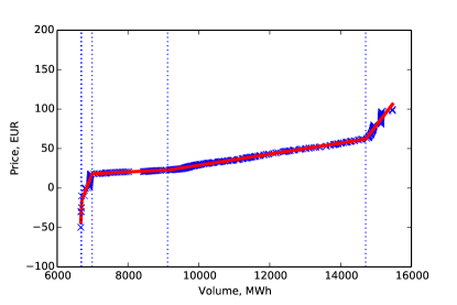
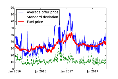
Figure 1: Left: typical offer curve in the French electricity market. Right: evolution of the daily mean and standard deviation of the offers by gas-fired power plants in the French electricity market.

Bidding function of gas-fired power plants

Since it is difficult to reconstruct the actual bidding function used by market participants, we use an ad hoc bidding function, satisfying our assumptions, which takes the following form:

$$F(x)=\mathbf{1}_{x>\epsilon}+\frac{1}{2}(1+\sin(-\pi/2+\pi x/\epsilon))\mathbf{1}_{0\leq x\leq\epsilon},$$

where $\epsilon$ is a parameter which we choose equal to $0.5$. This means that the conventional generators bid their full capacity as soon as the price is greater than the cost plus $0.5$ GBP. The actual choice of $\epsilon$ does not have a significant effect on the results.

Electricity demand projections.

The reference electricity consumption evolution scenario is taken from the British government projections. This reference provides a forecast of average annual electricity consumption up to 2035. In our model, the time step was fixed to 3 months and a distinction between peak (7AM-8PM, Mon-Fri) and off-peak demand has been made. To this end, we have used the high frequency electricity consumption data from gridwatch.co.uk to estimate the historical annual cycle and the historical peak/off-peak ratio. This enabled us to construct the projections of peak and off-peak consumption with the time step of 3 months. These are shown in Figure 2.

Distinction between peak and off-peak prices

For realistic modeling of electricity markets, it is essential to distinguish between peakload and baseload (off-peak) prices. In particular, the effect of renewable penetration on these two prices may be different. To this end, the simulations were carried out in a slightly modified version of the model, where peak and off-peak prices are computed separately, by matching the corresponding demand projection with the supply curve of the market, and the revenues of the agents are computed by adding up their revenues over peak and off-peak periods. All the theoretical developments carry over to this case, but we chose to present the single-price case in the paper to lighten the notation.

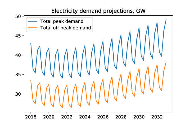
Figure 2: Electricity demand projections used in the simulation.

Simulation results

The first simulation illustrates the baseline case (with the parameters and modeling choices described above). We perform 300 iterations of the algorithm as described in Section 4, and monitor the gain increase from switching to the best response for renewable and conventional producers $\mathcal{E}^{C}(\omega^{(n)},\eta^{(n)})$ and $\mathcal{E}^{R}(\omega^{(n)},\eta^{(n)})$. Figure 3 shows the gain increase for the renewable and conventional producers in the baseline simulation: it can be seen that this quantity converges to zero at the rate $\frac{1}{n}$ where $n$ is the number of iterations. The final values for the baseline simulations correspond to a gain increase of about $0.001$ GBP per MW of installed capacity per hour for the conventional producers and $0.005$ GBP per MW of installed capacity per hour for the renewable producers, which is quite small compared to the price at which electricity is usually sold. Similar convergence rates and similar or smaller final values have been observed in other simulations described below.

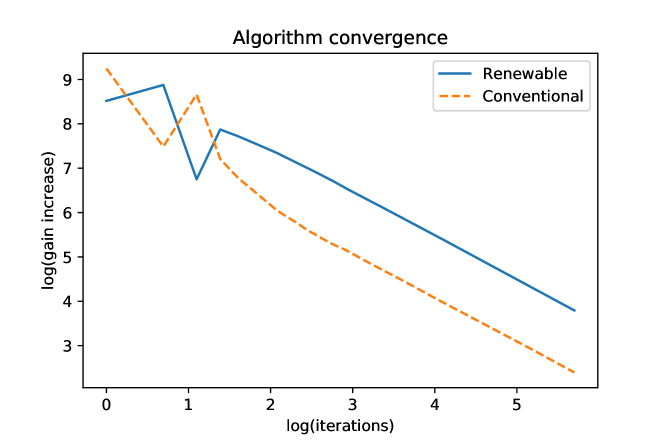
Figure 3: Convergence of the gain increase upon switching to the best response. The gain is given in million GBP for the entire sector.

In the second simulation, which we term Scenario 1, we assume that there is a 27% subsidy for renewable energy, bringing down the fixed cost of building a wind power plant to $1000$ GBP per kW of installed capacity. The other parameters are same as above.

In the third simulation, termed Scenario 2, we assume that the conventional producers receive a fixed payment of 10 GBP per KW of installed capacity per year. For comparison, the clearing prices at the UK T-4 capacity auctions were $19.4$ GBP/kW for 2018–2019, $18$ GBP/kW for 2019–2020, $22.5$ GBP/kW for 2020–2021 and $8.4$ GBP/kW for 2021-2022, see [26]. The 27% renewable subsidy is still in place.

Figure 4 shows the evolution of the conventional and renewable installed capacity in the three simulations. The corresponding price trajectories are shown in Figure 5. While in the baseline scenario, no new renewable capacity is installed, the 27% renewable subsidy (scenario 1) dramatically increases renewable installation, which practically doubles over the 15-year period. Notice that while the conventional capacity is reduced in the beginning of the 15-year period, the arrival of the renewable capacity is more gradual. This happens because of the form of the demand process (Figure 2) which grows in the second half of the 15-year period.

In terms of electricity prices, the main effect of the renewable subsidy is a reduction of the baseload price, especially during the winter months. On the other hand, the peakload electricity price in winter months increases compared to the baseline scenario. Thus, the renewable subsidy allows to decarbonize the electricity production, but may lead to higher peakload prices. This happens in our model because the conventional producers are strongly incentivised to leave the market. In scenario 2 this incentive is reduced (in our case this is achieved with capacity payments). As a result, the renewable penetration is slightly reduced, but the peakload price is considerably lower than in scenario 1, and also lower than in the baseline scenario. The baseload price, on the other hand, is much lower than in the baseline scenario, slightly higher than in scenario 1 in the summer months and similar to scenario 1 in the winter months.

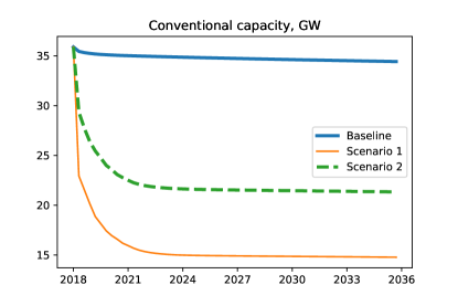
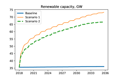
Figure 4: Evolution of conventional and renewable installed capacity in the three simulations. Scenario 1: renewable subsidy. Scenario 2: renewable subsidy and capacity payments for conventional plants.

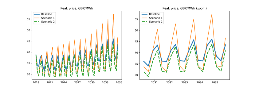
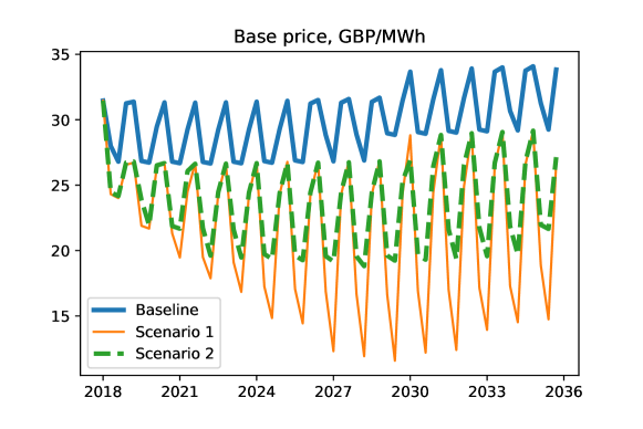
Figure 5: Evolution of the electricity price in the three simulations. Top left: peak price. Top right: peak price (zoom on the last 4 years). Bottom: base price. Scenario 1: renewable subsidy. Scenario 2: renewable subsidy and capacity payments for conventional plants.

We conclude that while renewable subsidies clearly lead to higher renewable penetration, this may entail a cost to the consumer in terms of higher peakload prices. In order to avoid rising prices, the renewable subsidies must be combined with market or off-market mechanisms ensuring that sufficient conventional capacity remains in place to meet the energy demand during peak periods.

6 Acknowledgement

Peter Tankov and René Aïd gratefully acknowledge financial support from the ANR (project EcoREES ANR-19-CE05-0042) and from the FIME Research Initiative.

Appendix A Technical proofs

We provide here the complete proof of Lemma 2.

Part i. Step 1. Introduce the function

$$L_{t}=\left(\overline{D}_{t}-\int_{\overline{\Omega}}{x(\bar{\eta}_{t}(dx)-\eta_{t}(dx))}\right)_{+}.$$

The price process satisfies

$$P_{t}(\omega_{t},\eta_{t})=\inf\{y\in[0,\overline{P}]:\int_{\Omega}F(y-x)\omega_{t}(dx)+F_{0}(y)\geq L_{t}\}\wedge\overline{P}.$$

We would like to show that $L$ has bounded variation on $[0,T]$. To this end, let $\psi:[0,T]\mapsto\mathbb{R}$ be a $C^{1}$ function. We first show that for all $t\in[0,T]$,

$$\left|\mathbb{E}\left[\int_{t}^{T}\psi^{\prime}(s)S^{t,x}_{s}ds\right]\right|\leq C\|\psi\|_{\infty}.$$

for some constant $C<\infty$. Indeed, by using Itô’s formula, we get:

$$\mathbb{E}\left[\int_{t}^{T}\psi^{\prime}(s)S_{s}^{t,x}ds\right]=\mathbb{E}\left[S_{T}^{s,x}\psi(T)-S_{t}^{s,x}\psi(t)\right]-\mathbb{E}\left[\int_{t}^{T}\psi(s)\bar{k}(\bar{\theta}-S_{s}^{t,x})ds\right].$$

Then, by using that the process $(S_{t}^{s,x})$ takes values between $0$ and $1$, the result easily follows. Now, we can consider the test function

$$u(t,x)=\mathbb{E}\left[\int_{t}^{T}\psi^{\prime}(s)S^{t,x}_{s}ds\right]+C\|\psi\|_{\infty}.$$

First note that, by construction, $u\geq 0$. Moreover, it is easy to check through explicit computation that $u\in C^{1,2}([0,T]\times\overline{\Omega})$. Moreover, $\overline{\Omega}$ is bounded and consequently, $\frac{\partial u}{\partial t}+\overline{\mathcal{L}}u=\psi^{\prime}(t)x$ is bounded on $[0,T]\times\overline{\Omega}$. Plugging this test function into the definition of $\overline{\mathcal{A}}(\eta_{0})$ yields

$$\int_{0}^{T}\psi^{\prime}(s)\int_{\overline{\Omega}}x\eta_{t}(dx)\leq 2C\|\psi\|_{\infty},$$

which means that the total variation of the mapping

$$t\mapsto\int_{\overline{\Omega}}x\eta_{t}(dx),$$

is bounded on $[0,T]$ by $2C$, and thus also $L_{t}$, has bounded variation on $[0,T]$.

Step 2. For a fixed $n$, define

$$F^{n}_{k}(t):=\int_{0}^{\overline{P}}F(k\overline{P}/n-x)\omega_{t}(dx)+F_{0}(k\overline{P}/n),\quad k=0,\dots,n.$$

We now would like to show that these functions have bounded variation on $[0,T]$, uniformly on $n,k$, in the sense that for every $n$ and every sequence of $C^{1}$ functions $\psi_{k}:[0,T]\mapsto\mathbb{R}$, $k=0,\dots,n$,

$$\sum_{k=0}^{n}\int_{0}^{T}F^{n}_{k}(t)\psi^{\prime}_{k}(t)dt\leq C\max_{0\leq t\leq T}\sum_{k=0}^{n}|\psi_{k}|,$$ (11)

where the constant $C$ does not depend on $k,n$. To this end, as above, we start with the following estimate, obtained by Itô formula and integration by parts, where to save space we omit the superscript $(t,x)$ of the process $C$.

$$\sum_{k=0}^{n}\mathbb{E}\left[\int_{t}^{T}\psi^{\prime}_{k}(s)F(k\overline{P}/n-C_{s})ds\right]$$

$$=\sum_{k=0}^{n}\mathbb{E}\Big{[}\int_{t}^{T}\psi^{\prime}_{k}(s)\Big{\{}F(k\overline{P}/n-x)-\int_{t}^{s}F^{\prime}(k\overline{P}/n-C_{r})k(\theta-C_{r})dr$$

$$\qquad+\frac{1}{2}\int_{t}^{s}F^{\prime\prime}(k\overline{P}/n-C_{r})\delta^{2}C_{r}dr\Big{\}}ds\Big{]}$$

$$=\sum_{k=0}^{n}(\psi_{k}(T)-\psi_{k}(t))F(k\overline{P}/n-x)$$

$$+\sum_{k=0}^{n}\mathbb{E}\Big{[}\int_{t}^{T}(\psi_{k}(T)-\psi_{k}(s))\Big{\{}-F^{\prime}(k\overline{P}/n-C_{s})k(\theta-C_{s})+\frac{1}{2}F^{\prime\prime}(k\overline{P}/n-C_{s})\delta^{2}C_{s}\Big{\}}ds\Big{]}$$

$$\leq C\max_{0\leq t\leq T}\sum_{k=0}^{n}\left|\psi_{k}(t)\right|,$$

because $F(k\overline{P}/n-x)$ and the terms in curly brackets in the last line above are bounded by a constant independent from $k$, $n$ and $x$ in view of the properties of $F$.

Now let us consider the test function

$$u(t,x)=\sum_{k=0}^{n}\mathbb{E}\left[\int_{t}^{T}\psi^{\prime}_{k}(s)F(k\overline{P}/n-C^{(t,x)}_{s})ds\right]+C\max_{0\leq t\leq T}\sum_{k=0}^{n}|\psi_{k}(t)|.$$

It is easy to check that it possesses the required regularity properties, and satisfies

$$\frac{\partial u}{\partial t}(t,x)+\mathcal{L}u(t,x)=\sum_{k=0}^{n}\psi^{\prime}_{k}(t)F(k\overline{P}/n-x).$$

Due to the boundedness property of the map $F$, we get that $\frac{\partial u}{\partial t}+\mathcal{L}u$ is bounded. Then, we plug it into the definition of $\mathcal{A}(\omega_{0})$ and since $\int_{0}^{\bar{P}}F(k{\overline{P}}/n-x)\omega_{t}(dx)=\int_{\Omega}F(k\overline{P}/n-x)\omega_{t}(dx)$ for all $t\in[0,T]$, the result follows.

Step 3. Let $\rho$ be a mollifier supported on $[-1,1]$, set $\rho_{m}(x):=m\rho(mx)$ and define

$$F^{n,m}_{k}(t):=\rho_{m}*F^{n}_{k}(t),$$

where $F^{n}_{k}$ is extended by zero value outside the interval $[0,T]$, so that $F^{n,m}_{k}$ is well defined on $[0,T]$. Let $\psi_{0},\dots,\psi_{n}$ be a sequence of test functions. Then, for every $m$ and for $k=0,\dots,n$,

$$\sum_{k=0}^{n}\int_{0}^{T}F^{n,m}_{k}(t)\psi_{k}^{\prime}(t)dt =\sum_{k=0}^{n}\int_{0}^{T}\psi_{k}^{\prime}(t)\int_{-1/m}^{1/m}F^{n}_{k}(t-s)\rho_{m}(s)ds\,dt$$

$$=\sum_{k=0}^{n}\int_{-1/m}^{1/m}\rho_{m}(s)ds\int_{0}^{T}\psi_{k}^{\prime}(t)F^{n}_{k}(t-s)dt$$

$$=\sum_{k=0}^{n}\int_{-1/m}^{1/m}\rho_{m}(s)ds\int_{0}^{T}\psi_{k}^{\prime}(t+s)F^{n}_{k}(t)dt$$

$$\leq C\max_{0\leq t\leq T}\sum_{k=0}^{n}|\psi_{k}(t)|\int_{-1/m}^{1/m}\rho_{m}(s)ds=C\max_{0\leq t\leq T}\sum_{k=0}^{n}|\psi_{k}(t)|,$$

where we extend $\psi_{k}$ by constants outside the interval $[0,T]$. The last inequality follows by Step 2. By integration by parts, then,

$$\sum_{k=0}^{n}\int_{0}^{T}\frac{d}{dt}F^{n,m}_{k}(t)\psi_{k}(t)dt\leq C\max_{0\leq t\leq T}\sum_{k=0}^{n}|\psi_{k}(t)|,$$

for a different constant $C$. Finally, by an approximation argument using the dominated convergence, this implies that

$$\int_{0}^{T}\max_{0\leq k\leq n}\left|\frac{d}{dt}F^{n,m}_{k}(t)\right|dt\leq C.$$

Step 4. By definition of $F_{0}$, $F^{n}_{k+1}(t)-F^{n}_{k}(t)\geq\frac{c\overline{P}}{n}$, $0\leq k\leq n-1$. Now for $y\geq 0$ and $0=x_{0}<x_{1}<\dots<x_{n}$, define the mapping $\Theta_{n}$ as follows.

$$\Theta_{n}(y,x_{0},\dots,x_{n})=\frac{\overline{P}}{n}\sum_{k=0}^{n-1}\frac{(y-x_{k})_{+}}{x_{k+1}-x_{k}}\wedge 1.$$

Then,

$$\frac{\partial\Theta_{n}}{\partial y} =\frac{\overline{P}}{n}\sum_{k=0}^{n-1}\frac{\mathbf{1}_{x_{k}\leq y<x_{k+1}}}{x_{k+1}-x_{k}},$$

$$\frac{\partial\Theta_{n}}{\partial x_{j}} =\frac{\overline{P}}{n}\frac{\mathbf{1}_{x_{j}\leq y<x_{j+1}}}{(x_{j+1}-x_{j})^{2}}(y-x_{j+1})-\frac{\overline{P}}{n}\frac{\mathbf{1}_{x_{j-1}\leq y<x_{j}}}{(x_{j}-x_{j-1})^{2}}(y-x_{j-1}).$$

Introduce the discretized price

$$P^{n}_{t}(\omega_{t},\eta_{t}):=\Theta_{n}(L_{t},F^{n}_{0}(t),\dots,F^{n}_{n}(t)).$$

Let $(L^{m}_{t})_{m\geq 1}$ be a sequence of $C^{\infty}$ functions approximating $L_{t}$ in the sense of Theorem 3.9 in [3], and let $F^{n,m}_{0},\dots,F^{n,m}_{n}$ be defined as in Step 3. Let $\phi:[0,T]\mapsto\mathbb{R}$ be a $C^{1}$ function. Then,

$$\int_{0}^{T}\phi^{\prime}(t)P^{n}_{t}(\omega_{t},\eta_{t})dt =\lim_{m\to\infty}\int_{0}^{T}\phi^{\prime}(t)\Theta_{n}(L^{m}_{t},F^{n,m}_{0}(t),\dots,F^{n,m}_{n}(t))dt$$

$$\leq 2\|\phi\|_{\infty}\overline{P}+\lim_{m\to\infty}\int_{0}^{T}\phi(t)\left\{\frac{\partial\Theta_{n}}{\partial y}\frac{d}{dt}L^{m}_{t}+\sum_{j=0}^{n}\frac{\partial\Theta_{n}}{\partial x_{j}}\frac{d}{dt}F^{n,m}_{j}(t)\right\}dt$$

$$\leq 2\|\phi\|_{\infty}\overline{P}+\|\phi\|_{\infty}\|\frac{\partial\Theta_{n}}{\partial y}\|_{\infty}\lim_{m}\int_{0}^{T}|\frac{d}{dt}L^{m}_{t}|dt$$

$$+\|\phi\|_{\infty}\lim_{m}\int_{0}^{T}\sum_{k}|\frac{\partial\Theta_{n}}{\partial x_{k}}|\max_{k}|\frac{d}{dt}F^{n,m}_{k}(t)|dt.$$

Since $\frac{\partial\Theta_{n}}{\partial x_{k}}(t)\neq 0$ for only two $k$, we deduce that $|\frac{\partial\Theta_{n}}{\partial x_{k}}(t)|\leq 2c$ and therefore,

$$\int_{0}^{T}\phi^{\prime}(t)P^{n}_{t}(\omega_{t},\eta_{t})dt \leq 2\|\phi\|_{\infty}\overline{P}+\|\phi\|_{\infty}\|\frac{\partial\Theta_{n}}{\partial y}\|_{\infty}\lim_{m}\int_{0}^{T}|\frac{d}{dt}L^{m}_{t}|dt$$ (12)

$$+\|\phi\|_{\infty}\|\sum_{k}\frac{\partial\Theta_{n}}{\partial x_{k}}\|_{\infty}\lim_{m}\int_{0}^{T}\max_{k}|\frac{d}{dt}F^{n,m}_{k}(t)|dt$$

$$\leq 2\|\phi\|_{\infty}\overline{P}+c\|\phi\|_{\infty}\lim_{m}\int_{0}^{T}|\frac{d}{dt}L^{m}_{t}|dt$$

$$+2c\|\phi\|_{\infty}{\lim_{m}\int_{0}^{T}\max_{k}|\frac{d}{dt}F^{n,m}_{k}(t)|dt}\leq C\|\phi\|_{\infty}.$$

for some constant $C$, by the estimates provided in Step 3. This shows that the total variation of $P^{n}$ on $[0,T]$ is bounded uniformly on $n$. On the other hand, by construction, it is easy to see that $|P^{n}_{t}-P_{t}|\leq\frac{\overline{P}}{n}$, so that $P_{t}^{n}\to P_{t}$ as $n\to\infty$ for all $t$. Then, by passing to the limit in (12), we can conclude that $P_{t}$ has bounded variation on $[0,T]$.

Part ii. By the arguments of the first part of the proof, the mappings

$$t\mapsto\int_{\overline{\Omega}}x\eta^{m}_{t}(dx)$$

and, for every $n$ and $k=0,\dots,n$,

$$t\mapsto\int_{\Omega}F(k\overline{P}/n-x)\omega^{m}_{t}(dx)+F_{0}(k\overline{P}/n)$$

have variation bounded uniformly on $m$. Therefore, one can find a subsequence $(m_{q})_{q\geq 1}$ along which these mappings converge to certain limits in $L^{1}([0,T])$. Moreover, since $\overline{\Omega}$ is bounded, in view of weak convergence of measures, for any bounded continuous function $\phi:[0,T]\mapsto\mathbb{R}$,

$$\lim_{m}\int_{0}^{T}\phi(t)\int_{\overline{\Omega}}x\eta^{m}_{t}(dx)=\int_{0}^{T}\phi(t)\int_{\overline{\Omega}}x\eta^{*}_{t}(dx),$$

which means that also

$$\int_{\overline{\Omega}}x\eta^{m_{q}}_{\cdot}(dx)\xrightarrow{L^{1}([0,T])}\int_{\overline{\Omega}}x\eta^{*}_{\cdot}(dx).$$

Similar arguments show that

$$\int_{\Omega}F(k\overline{P}/n-x)\omega^{m_{q}}_{\cdot}(dx)\xrightarrow{L^{1}([0,T])}\int_{\Omega}F(k\overline{P}/n-x)\omega^{*}_{\cdot}(dx).$$

Since the mapping $\Theta_{n}$ introduced at Step 4 is Lipschitz, this implies that the sequence of discretized prices $P^{n}_{\cdot}(\omega^{m_{q}}_{t},\eta^{m_{q}}_{\cdot})$ also converges in $L^{1}([0,T])$ to the discretized price $P^{n}_{\cdot}(\omega^{*}_{\cdot},\eta^{*}_{\cdot})$. On the other hand, we have seen that $|P^{n}_{t}(\omega^{*}_{t},\eta^{*}_{t})-P_{t}(\omega^{*}_{t},\eta^{*}_{t})|\leq\frac{\overline{P}}{n}$. Therefore, for any $\varepsilon>0$, by taking $n\geq\frac{3\overline{P}T}{\varepsilon}$ and then choosing $q$ such that

$$\|P^{n}_{\cdot}(\omega^{m_{q}}_{\cdot},\eta^{m_{q}}_{\cdot})-P^{n}_{\cdot}(\omega^{*}_{\cdot},\eta^{*}_{\cdot})\|_{L^{1}}\leq\frac{\varepsilon}{3},$$

we have that

$$\|P_{\cdot}(\omega^{m_{q}}_{\cdot},\eta^{m_{q}}_{\cdot})-P_{\cdot}(\omega^{*}_{\cdot},\eta^{*}_{\cdot})\|_{L^{1}}\leq\varepsilon,$$

which proves the second part of the lemma.

References

• [1] R. Aïd, L. Li, and M. Ludkovski, Capacity expansion games with application to competition in power generation investments, Journal of Economic Dynamics and Control, 84 (2017), pp. 1–31.
• [2] C. Alasseur, I. Ben Tahar, and A. Matoussi, An extended mean field game for storage in smart grids, arXiv preprint arXiv:1710.08991, (2017).
• [3] L. Ambrosio, N. Fusco, and D. Pallara, Functions of bounded variation and free discontinuity problems, vol. 254, Clarendon Press Oxford, 2000.
• [4] F. Bagagiolo and D. Bauso, Mean-field games and dynamic demand management in power grids, Dynamic Games and Applications, 4 (2014), pp. 155–176.
• [5] M. Ben Alaya and A. Kebaier, Parameter estimation for the square root diffusions: ergodic and nonergodic cases, Stochastic Models, 28, Iss.4 (2012), pp. 609–634.
• [6] D. Benatia, Functional econometrics of multi-unit auctions: An application to the New York electricity market, (2018). Working paper.
• [7] C. Bertucci, Optimal stopping in mean field games, an obstacle problem approach, Journal de Mathématiques Pures et Appliquées, 120 (2018), pp. 165–194.
• [8] P. C. Bhagwat, A. Marcheselli, J. C. Richstein, E. J. Chappin, and L. J. De Vries, An analysis of a forward capacity market with long-term contracts, Energy policy, 111 (2017), pp. 255–267.
• [9] G. Bouveret, R. Dumitrescu, and P. Tankov, Mean-field games of optimal stopping: a relaxed solution approach, SIAM Journal on Control and Optimization, (to appear).
• [10] C. Byers, T. Levin, and A. Botterud, Capacity market design and renewable energy: Performance incentives, qualifying capacity, and demand curves, The Electricity Journal, 31 (2018), pp. 65–74.
• [11] S. Clò, A. Cataldi, and P. Zoppoli, The merit-order effect in the Italian power market: The impact of solar and wind generation on national wholesale electricity prices, Energy Policy, 77 (2015), pp. 79–88.
• [12] R. Couillet, S. M. Perlaza, H. Tembine, and M. Debbah, A mean field game analysis of electric vehicles in the smart grid, in 2012 Proceedings IEEE INFOCOM Workshops, IEEE, 2012, pp. 79–84.
• [13] S. N. Ethier and T. G. Kurtz, Markov processes: characterization and convergence, vol. 282, John Wiley & Sons, 2009.
• [14] N. Fabra, A primer on capacity mechanisms, Energy Economics, 75 (2018), pp. 323–335.
• [15] D. Gomes and S. Patrizi, Obstacle mean-field game problem, Interfaces and Free Boundaries, 17 (2015), pp. 55–68.
• [16] D. Gomes and J. Saúde, Mean field games models – a brief survey, Dynamic Games and Applications, 4 (2014), pp. 110–154.
• [17]  , A mean-field game approach to price formation, Dynamic Games and Applications, (2020), pp. 1–25.
• [18] C. Gouriéroux and P. Valéry, Estimation of a Jacobi process, Preprint, (2004).
• [19] A. Henriot and J.-M. Glachant, Melting-pots and salad bowls: The current debate on electricity market design for integration of intermittent res, Utilities Policy, 27 (2013), pp. 57–64.
• [20] International Energy Agency, Energy Technology Prospectives Report, June 2017.
• [21] Leigh Fisher Jacobs, Electricity generation costs and hurdle rates, tech. rep., Department of Energy and Climate Change, 2016.
• [22] R. Kiesel and F. Paraschiv, Econometric analysis of 15-minute intraday electricity prices, Energy Economics, 64 (2017), pp. 77–90.
• [23] J.-M. Lasry and P.-L. Lions, Mean field games, Japanese journal of mathematics, 2 (2007), pp. 229–260.
• [24] T. Levin and A. Botterud, Electricity market design for generator revenue sufficiency with increased variable generation, Energy Policy, 87 (2015), pp. 392–406.
• [25] B. Murray, The paradox of declining renewable costs and rising electricity prices, Forbes, (2019).
• [26] Department of Business Energy and Industrial Strategy, Capacity market five-year review 2014–2019, tech. rep., UK Government, 2019.
• [27] V. Rious, Y. Perez, and F. Roques, Which electricity market design to encourage the development of demand response?, Economic Analysis and Policy, 48 (2015), pp. 128–138.
• [28] S. Schwenen, Strategic bidding in multi-unit auctions with capacity constrained bidders: the New York capacity market, The RAND Journal of Economics, 46 (2015), pp. 730–750.
• [29] R. Takashima, M. Goto, H. Kimura, and H. Madarame, Entry into the electricity market: Uncertainty, competition, and mothballing options, Energy Economics, 30 (2008), pp. 1809–1830.
• [30] R. C. Thomson and G. P. Harrison, Life cycle costs and carbon emissions of onshore wind power, tech. rep., University of Edinburgh, 2015.
• [31] A. Weidlich and D. Veit, A critical survey of agent-based wholesale electricity market models, Energy Economics, 30 (2008), pp. 1728–1759.