Hidden velocity ordering in dense suspensions of self-propelled disks

Abstract

Recent studies of the phase diagram for spherical, purely repulsive, active particles established the existence of a transition from a liquid-like to a solid-like phase analogous to the one observed in colloidal systems at thermal equilibrium, in particular in two dimensions an intermediate hexatic phase is observed. Here, we present evidence that the active dense phases (solid, hexatic and liquid) exhibit interesting dynamical anomalies. First, we unveil the growth - with density and activity - of ordered domains where the particles’ velocities align in parallel or vortex-like patches. Second, when activity is strong, the spatial distribution of kinetic energy becomes heterogeneous with high energy regions correlated to defects of the crystalline structure. This spatial heterogeneity is accompanied by temporal intermittency, with sudden peaks in the time-series of kinetic energy. The observed dynamical anomalies are not present in a dense equilibrium system and cannot be detected by considering only the structural properties of the system.

I Introduction

The dynamics of colloidal particles at high densities has been largely explored, theoretically, numerically and experimentally, in the last decades Löwen (1994); Gasser (2009). At thermodynamic equilibrium, the Mermin-Wagner theorem rules out the existence of a crystalline phase in two dimensional systems, characterized by long-range translational order Mermin and Wagner (1966); Mermin (1968). As shown by Halperin, Nelson Halperin and Nelson (1978), and Young Young (1979), in two dimensions the melting transition proceeds via two continuous Berezinskii-Kosterlitz-Thouless Berezinsky (1970); Kosterlitz and Thouless (1973) transitions driven by topological defects, i.e., a hexatic-liquid transition, with a quasi-long range orientational order, and a solid-hexatic transition, characterized by quasi-long range translational order and long-range orientational order Young (1979); Gasser et al. (2010). Density and temperature are the control parameters to move from liquid to hexatic and to solid-like aggregation phases. This scenario has been verified employing dense suspensions of equilibrium colloids Zahn et al. (1999); Dullens et al. (2017).

Recently, the study of two dimensional systems of self-propelled particles at high packing fractions has attracted the attention of the active matter community Marchetti et al. (2013); Gompper et al. (2020), since it may offer interesting engineering applications, for instance, in the design of new materials Bechinger et al. (2016). Although most of the experimental studies have so far focused on the low densities regime, some novel experiments have investigated Janus particles also in the case of very dense suspensions Klongvessa et al. (2019). Another interesting class of high-density non-equilibrium systems is represented by driven granular media where mono-disperse polar grains under shaking Deseigne et al. (2010) display persistent motion. It is also worth to mention some recent studies of artificial microswimmers at such densities Briand and Dauchot (2016), revealing an intriguing experimental scenario for non-equilibrium aggregation. Specimens of active matter systems at very high densities are very interesting also in the biological realm. Typical examples are tissues composed of highly packed eukaryotic cells. Particular attention has been devoted to the dynamics of confluent monolayers Angelini et al. (2011); Garcia et al. (2015), which slows down as density increases. More recently, an amorphous “solidification” process has been investigated during the process of vertebrate body axis elongation Mongera et al. (2018), where cells become solid-like.

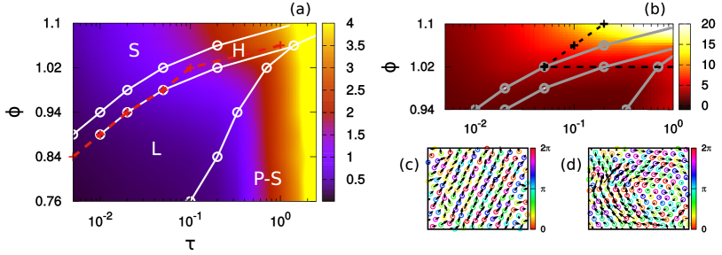
Figure 1: Dynamical phase diagram. In panel (a), we plot the phase diagram as a function of $\tau$ and $\phi$, coloring each region depending on the size of the aligned domains, quantified by the parameter $R/\sigma$. The symbols S, H, L, and P-S denote solid, hexatic, liquid and phase-separated phases, respectively, and are separated by solid lines. The dashed red line is obtained monitoring the pair correlation function, $g(r)$. Panel (b) focuses on the top region of the phase diagram and is colored depending on the correlation length, $\ell$, of the spatial velocity correlation. The dashed black line delimits the regions where kinetic energies show an intermittent phenomenology. Panels (c) and (d) show two zooms of the snapshot configuration realized at $\phi=1.1$ and $\tau=1$. Colors encode the orientation of the self-propulsion while the black arrows represent the velocity vectors. Panel (c) shows an aligned domain, while panel (d) a vortex-like structure in the pattern of the particles’ velocities. Simulations are obtained with $v_{0}=50$ and the inter-particles interaction discussed in the main text.

Theoretical approaches in the statistical physics of active matter focus on simplified models of self-propelled particles, the Active Brownian Particle (ABP) being one of the most studied. Despite the existence of a vast literature concerning the regime of moderate packing fractions, ABP dynamics in the high-density regime is by far less explored. For instance, active crystallization is studied in Ref. Bialké et al. (2012), where a a shift of the liquid-solid transition line towards larger densities with respect to the Brownian counterpart is revealed. Besides, this transition is accompanied by a true non-equilibrium phenomenon: liquid and solid phases are separated by a region where the suspension is globally ordered but bubbles of “liquid” still persist. A more detailed analysis revealed the occurrence of traveling crystals Menzel and Löwen (2013); Menzel et al. (2014), accompanied by the transition to rhombic, square and even lamellar patterns. This phenomenology has been recently confirmed by experiments realized with vibrating granular disks Briand et al. (2018).

The construction of the phase diagram of the ABP model Digregorio et al. (2018); Cugliandolo et al. (2017); Stenhammar et al. (2014), follows the idea that its behavior Klamser et al. (2018) for small active forces resembles that of passive Brownian particles with the occurrence of “gas-like”, “liquid-like”, “hexatic-like” and “solid-like” phases, with a shift of the transition lines towards larger densities when activity increases Digregorio et al. (2018); Klamser et al. (2018). On the contrary, for large self-propulsion (but moderate densities) an unexpected phenomenon occurs: the system phase separates even in the absence of attractive interactions Redner et al. (2013); Buttinoni et al. (2013); Palacci et al. (2013); Bialké et al. (2015a); Ginot et al. (2018); Siebert et al. (2017); Cugliandolo et al. (2017); Speck (2016); Chiarantoni et al. (2020) (the so-called Motility Induced Phase Separation (MIPS) Fily and Marchetti (2012); Cates and Tailleur (2015); Gonnella et al. (2015); Ma et al. (2020)). Differently, at high densities but far from equilibrium, “standard” crystallization seems to occur Bialké et al. (2012); Digregorio et al. (2018). The general picture suggested by these studies is that the high-density equilibrium scenario extends, qualitatively identical, to active systems, with the only difference that self-propulsion may destabilize the ordered phases or induce a phase-separation.

Some other studies suggest that active dense phases in the MIPS region display a richer picture with respect to passive phases in the coexistence region. For instance, a quite different behavior can be found by analyzing the pressure Solon et al. (2015a, b) and the interfacial tension between the gas and the cluster phase Bialké et al. (2015b); Patch et al. (2018). Recently, the study of the particles’ velocities has revealed unexpected features which are certainly absent in equilibrium fluids, e.g. the different kinetic temperatures inside and outside a cluster Mandal et al. (2019), and the spontaneous alignment of velocities in the phase-separated regime Caprini et al. (2020).

I.1 Summary of results

Our main findings can be summarised by the introduction of dynamical information about the particles’ velocities into the structural phase diagram, as shown in Fig. 1. The phase diagram concerns the two-dimensional high-density regimes (both homogeneous and phase-separated), with two main control parameters: the persistence time, $\tau$, of the active force (which is proportional to the Péclet number and inversely proportional to the rotational diffusivity) and the packing fraction, $\phi$. We recall the definition of $\phi=N\sigma^{2}\pi/4L^{2}$, being $N/L^{2}$ the number density and $\sigma$ the particles’ diameter. Our “augmented” phase diagram challenges the widespread idea that the structural properties alone are enough to describe the dense phases of self-propelled particles, and suggests that a richer picture is obtained by including velocity correlations which, in turn, represent an exquisitely off-equilibrium feature of active systems.

Panel (a) of Fig. 1 portrays the phase diagram as a function $\phi$ and $\tau$, which reproduces Digregorio et al. (2018), with three homogeneous phases, i.e. the solid phase (S), the hexatic phase (H) and the liquid phase (L), and a non-homogeneous regime with MIPS-like phase coexistence (P-S), see Sec. II B for details. Our first finding is that the alignment of particles’ velocities discovered in Caprini et al. (2020) in the P-S regime is observed also in the homogeneous liquid, hexatic and solid phases. Particles’ velocities form patterns arranging in aligned or vortex-like domains, as shown by the arrows in panels (c) and (d) of Fig. 1, even if the orientation of self-propulsion has negligible order (see color coding in the same panels). The size of aligned domains - quantified by $R$, defined later, encoded by colors in panel (a) - grows as $\tau$ and $\phi$ increase, as discussed in detail in Sec. III A. In the homogeneous liquid configurations, the size of the aligned velocity domains is rather small as a result of the absence of translational order, at variance with the solid (denser) case where the sizes reach large values. In the non-homogeneous configurations, only the growth of $\tau$ induces the increase of the correlation length as a result of density saturation. We recall that order in the velocity field is absent in any passive Brownian suspension, even at high densities: it is, in fact, a pure non-equilibrium feature due to the presence of propulsion forces in the active dynamics. Interestingly, a similar effect is also observed in fluidized granular materials, but it is caused by the presence of dissipative interactions Puglisi et al. (2012); Manacorda (2018); Plati et al. (2019). Fig. 1 (b) focuses on the top part (largest densities) of the phase diagram: the color encodes different information here, i.e. the correlation length $\ell$ of the spatial velocity correlation which takes into account also kinetic energy (square modulus of velocity) and not only the orientation of the velocity vectors as in the case of $R$ in panel (a). We observe that $\ell$ increases in the solid phase and saturates in the hexatic or liquid phases, because of the absence of both translational and/or orientational order (it increases again in the phase-separated regime as explained in detail in Sec. III C). In the same panel, a dashed black line delimits a region where heterogeneous spatial distributions and temporal intermittent behaviors of the kinetic energy are observed: interestingly, these anomalies in the kinetic energy field are correlated to the structural defects of the crystal arrangement (see details in Sec. III B).

The article is structured as follows: in Sec. II, we introduce the ABP model for interacting self-propelled particles, summarizing the structural properties of the system. In Sec. III, we present a detailed study of all the dynamical anomalies in the velocity orientation, velocity vector and kinetic energy fields, correlating these anomalies to the different structural properties of the system. A theoretical approach is also presented in Sec. III C that allows us to predict the features of the spatial correlation functions of the velocity field. Section IV is devoted to conclusions and perspectives.

II The system of interacting self-propelled particles

We study a system of $N$ interacting ABP disks in two dimensions moving in a fluid at high viscosity (low-Reynolds number). We neglect both hydrodynamic interactions among the particles and inertial terms Bechinger et al. (2016). The center of mass of each disk, $\mathbf{x}_{i}$, evolves according to the following stochastic differential equation:

$$\gamma\dot{\mathbf{x}}_{i}=\mathbf{F}_{i}+\mathbf{f}^{a}_{i}\,,$$ (1)

where $\gamma$ is the drag coefficient of the fluid and the effect of the thermal noise due to the solvent is assumed to be much smaller than the effect due to the random active force $\mathbf{f}^{a}_{i}$ Bechinger et al. (2016). The term $\mathbf{F}_{i}$ represents the force contribution due to steric interactions, such that, $\mathbf{F}_{i}=-\nabla_{i}U_{tot}$, being $U_{tot}=\sum_{i<j}U(|{\mathbf{x}}_{ij}|)$, with ${\mathbf{x}}_{ij}=\mathbf{x}_{i}-\mathbf{x}_{j}$.

Following several studies in the literature Redner et al. (2013); Caprini et al. (2020), we choose $U(r)$ as a truncated and shifted Lennard-Jones potential:

$$U(r)=\begin{cases}&4\epsilon\left[\left(\dfrac{\sigma}{r}\right)^{12}-\left(\dfrac{\sigma}{r}\right)^{6}\right]+\epsilon,\quad\,\,r\leq 2^{1/6}\sigma\\ &0\,,\qquad\qquad\qquad\qquad\qquad\quad r\geq 2^{1/6}\sigma\,.\end{cases}$$ (2)

The constant $\sigma$ represents the nominal particle diameter while $\epsilon$ is the typical energy scale of the interaction. For numerical convenience, both these parameters are set to one in the simulations. Even in very packed configurations, each particle can only interact with its first neighbors due to the truncated potential.

The self-propulsion force, $\mathbf{f}^{a}_{i}=\gamma v_{0}\mathbf{n}_{i}$, evolves with ABP dynamics: $v_{0}$ is the modulus of the speed induced by the self-propulsion for a force-free particle, $\mathbf{n}_{i}$ is a unit vector of components $(\cos{\theta_{i}},\sin{\theta_{i}})$. The orientational angle, $\theta_{i}$, performs angular diffusive motion described by:

$$\dot{\theta}_{i}=\sqrt{2D_{r}}\,\xi_{i}\,,$$ (3)

where $\xi_{i}$ is a white noise with unit variance and zero average. The constant $D_{r}$ represents the rotational diffusion coefficient and its inverse defines the typical relaxation time, $\tau=1/D_{r}$, of the active force Farage et al. (2015).

We remark that no explicit aligning force is included in the present model at variance with Vicsek-like models where particles’ velocities are forced to align to the mean orientation of surrounding particles’ velocities Vicsek and Zafeiris (2012); Grégoire and Chaté (2004). Thus, in contrast with Vicsek-like models, the dynamics (1) does not produce any polarization of the directors $\mathbf{n}_{i}$. We also avoid employing any form of self-alignment between the particle velocity and the self-propulsion force responsible for orientation-velocity ordering as recently proposed in Lam et al. (2015); Giavazzi et al. (2018).

II.1 The effective velocity dynamics of the particle

In order to obtain theoretical predictions and interpret the results, following Caprini et al. (2020), it is useful to switch from the set of variables $\{\mathbf{x}_{i},\mathbf{f}^{a}_{i}\}$ to the transformed variables $\{\mathbf{x}_{i},\mathbf{v}_{i}\}$ eliminating the self-propulsions in favor of the particles’ velocities, $\mathbf{v}_{i}=\dot{\mathbf{x}}_{i}$. We underline that the vectors $\mathbf{f}^{a}_{i}$ and $\mathbf{v}_{i}$ are not aligned, because of the interaction force $\mathbf{F}_{i}$. This is true, in particular, at high densities. The transformed dynamics reads:

$$\dot{\mathbf{x}}_{i} =\mathbf{v}_{i}$$ (4)

$$\tau\gamma\dot{\mathbf{v}}_{i} =-\gamma\sum_{j=1}^{N}{\bm{\Gamma}}_{ij}({\mathbf{r}}_{ij})\mathbf{v}_{j}+\mathbf{F}_{i}+\tau\gamma\mathbf{k}_{i}$$ (5)

where both $\mathbf{v}_{i}$ and $\mathbf{x}_{i}$ belong to the plane $xy$ and $\mathbf{r}_{ij}=\mathbf{x}_{i}-\mathbf{x}_{j}$. Each term $\bm{\Gamma}_{ij}$ is a $2\times 2$ matrix, whose elements are:

$$\Gamma_{ij}^{\alpha\beta}({\mathbf{r}}_{ij})=\delta_{ij}\delta_{\alpha\beta}+\frac{\tau}{\gamma}\nabla_{i\alpha}\nabla_{j\beta}U(|{\mathbf{r}}_{ij}|)\,,$$ (6)

where Latin indices identifying the particles assume values $i,j=1,N$ while the Greek indices stand for spatial components $(x,y)$. The last addend in Eq. (5), $\mathbf{k}_{i}$, is a noise term which reads:

$$\mathbf{k}_{i}=v_{0}\sqrt{2/\tau}\,\bm{\xi}_{i}\times{\mathbf{n}}_{i}=v_{0}\sqrt{2/\tau}\,\bm{\xi}_{i}\times\frac{\gamma\mathbf{v}_{i}-\mathbf{F}_{i}}{\gamma v_{0}}\,.$$ (7)

$\bm{\xi}_{i}$ is the stochastic vector with components $(0,0,\xi_{i})$ normal to plane of motion. At variance with the dynamics of $\mathbf{f}^{a}_{i}$, the modulus of $\mathbf{v}_{i}$ is not constant because of the term $\propto\bm{\xi}_{i}\times\mathbf{F}_{i}$. The result can be easily generalized to the case of finite thermal noise, as shown in Appendix A, using the strategy of Caprini and Marconi (2018).

The deterministic part of Eq. (5) represents the dynamics of an underdamped passive particle under the action of a space-dependent friction. Indeed, the first term in the right-hand side of Eq. (5) can be split into a contribution $-\gamma\Gamma_{ii}\mathbf{v}_{i}$, representing a generalized Stokes force acting on the $i$-th particle plus a second contribution, $-\gamma\sum_{j\neq i}^{N}{\Gamma}_{ij}({\mathbf{r}}_{ij})\mathbf{v}_{j}$, which depends on particles’ relative positions and velocities and vanishes in a passive system.

The ABP equation (5) for the velocity strongly resembles the analogous equation of another schematic model of self-propelled particles, namely the Active Ornstein-Uhlenbeck model (AOUP) Marconi and Maggi (2015); Marconi et al. (2017, 2016); Fodor et al. (2016); Wittmann et al. (2019); Berthier et al. (2019); Caprini et al. (2019a); Woillez et al. (2019); Caprini and Marconi (2019); Maggi et al. (2017). Such a connection has recently been established in some studies Caprini et al. (2019b); Das et al. (2018): the only difference between ABP and AOUP arises from the noise term $\mathbf{k}_{i}$. In the latter case, $\mathbf{k}_{i}$ is a simple white noise acting on the velocity as an effective thermal bath. On the other hand, in ABP, $\mathbf{k}_{i}$ is perpendicular to $\mathbf{n}_{i}$, the orientation of the active force, and is a multiplicative noise since its amplitude depends both on $\mathbf{v}_{i}$ and $\mathbf{F}_{i}$ through the unit vector $\mathbf{n}_{i}$. Also notice that (since $\xi_{i}$ has unit variance and $\mathbf{n}$ is a unit vector) the variances of the ABP and AOUP noises coincide, being $v_{0}^{2}/\tau$. We underline that, upon fixing $v_{0}$, the noise variance decreases in the large persistence regime.

II.2 Known results and positional order

In the present Section, we illustrate the phase diagram for the values of the control parameters $\phi$ and $\tau$ (at fixed $v_{0}$) explored in this work. Our results are obtained by means of numerical solutions of Eqs. (1) in a square domain of size $L$ under periodic boundary conditions. In the considered interval of packing fractions ($\phi\in[0.78,1.1]$), a suspension of passive Brownian particles exhibits liquid, hexatic and solid phase depending on the temperature. Our ABP phase diagram is consistent with the findings of Di Gregorio et al. Digregorio et al. (2018). As shown by these authors, as $\tau$ is increased the liquid-hexatic and the hexatic-solid boundaries shift to larger values of $\phi$ and the hexatic region of the phase diagram is enlarged with respect to the passive equilibrium picture.

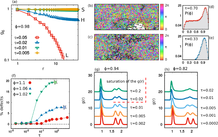
Figure 2: Structural properties. Panel (a): $g_{6}(r)$ at $\phi=0.98$ for different values of $\tau$, as reported in the caption, exploring the different structural phases: the symbols S, H and L refer to the almost-solid, hexatic and liquid phases, respectively. Panel (b), (c) are two snapshot configurations where colors denote the orientation of the particles, namely $\theta$, while panels (d) and (e) show the distribution of the packing fraction, $P(\hat{\phi})$, corresponding to the two configurations. In panel (f), we study the fraction of defects in the whole box vs $\tau$ for three different values of the densities as illustrated in the caption. The colored stars sign the value of $\tau$ at which the system becomes non-homogeneous. Panels (g) and (h) show a set of $g(r)$ obtained at different $\tau$ for $\phi=0.94,0.82$, respectively. Each curve is shifted along $y$ for presentation reasons. Simulations are always realized with $v_{0}=50$ and the interaction discussed in the text.

When the persistence is smaller than the time-scale associated with the potential, i.e. when $\tau\ll(\nabla\cdot\mathbf{F}(\bar{x})/\gamma)^{-1}$, (being $\bar{x}$ the average distance between neighboring particles, which is fixed by the density in any homogeneous configurations) we expect the same behavior as passive Brownian particles Caprini et al. (2019c): particles are homogeneously distributed in the box and arranged in the solid, hexatic or liquid phases, as shown in Digregorio et al. (2018), depending on the interplay between $\phi$ and $\tau$. In this regime, the active force acts as a thermal bath with effective diffusivity $\sim v_{0}^{2}\tau$. Thus, the growth of $\tau$, at fixed $v_{0}$, can be mapped in the increase of the effective diffusivity in the corresponding Brownian system. Depending on the interplay between $\phi$ and the effective temperature, the system explores liquid, hexatic or solid phases. The structural properties are detected monitoring the behavior of the orientational order parameter Cugliandolo et al. (2017); Cugliandolo and Gonnella (2018), $\psi_{6}\left(\mathbf{x}_{i}\right)$, defined as $\psi_{6}\left(\mathbf{x}_{i}\right)=\sum_{j}e^{6i\alpha_{ij}}/N_{i}$, where $\alpha_{ij}$ is the angle - with respect to $x$ axis - of the segment joining the $i$-th and the $j$-th particle and the sum is restricted to the first neighbors of the particle $i$, namely $N_{i}$. In particular, we focus on the correlation function, $g_{6}(r=|\mathbf{x}_{i}-\mathbf{x}_{j}|)=\langle\psi_{6}(\mathbf{x}_{i})\psi_{6}^{*}(\mathbf{x}_{j})\rangle/\langle\psi_{6}^{2}(\mathbf{x}_{j})\rangle$, to distinguish between different phases. While $g_{6}(r)$ is roughly constant with the distance in the solid phase, it decays as an inverse power-law in the hexatic phase. Differently, in the liquid phase, $g_{6}(r)$ shows an exponential decay. Examples of the different decays of $g_{6}(r)$ in the three structural phases are shown in Fig. 2 (a).

In addition, we also measure the pair correlation function, $g(r)$. At high density, the arrangement of particles is close to the hexagonal lattice, so that the peaks of the $g(r)$ are placed at positions $\bar{x},\sqrt{3}\bar{x},2\bar{x},\sqrt{7}\bar{x},...$ and so on, where $\bar{x}$ is the typical distance between neighboring particles, fixed by the density in any homogeneous configurations. It is worthy to note that $\bar{x}$ is quite smaller than $\sigma$, meaning that particles climb on the interacting potential due to the large densities. Each particle only interacts with its six neighbors due to the truncated nature of $U(r)$. In analogy with an equilibrium system, one can roughly identify the liquid phase with the parameter region where the second peak of $g(r)$ is not split. We see that for all values of the packing fraction, the peaks of the $g(r)$ decrease as $\tau$ is increased, in agreement with the interpretation of the self-propulsion in terms of effective diffusivity: fluidization occurs. The $g(r)$ is shown in panels (g) and (h) of Fig. 2 for several values of $\tau$ and two densities $\phi=0.94,0.82$, respectively: at high density (g), the system maintains a split second peak, while at moderate density (h), the system shows a transition - increasing $\tau$ - towards a single second peak where a liquid-like structure occurs Caprini et al. (2019c). Increasing $\tau$ beyond some threshold value (that depends on $\phi$) denoted as a red dotted line in panel (g), the curves representing $g(r)$ saturate, meaning that the internal structure is no more influenced by the value of $\tau$. On the other hand, the shape of $g(r)$ changes towards less fluid configurations where the system shows phase-separation or inhomogeneities. This is not a surprise since, in those cases, particles in the clusters attain a more compact configuration.

The boundary line between the homogeneous and inhomogeneous (phase-separated) regimes is obtained by monitoring the distribution of the local packing fraction, $P(\hat{\phi})$, shown in panels (d) and (e) of Fig. 2 for two different configurations at the same densities and different $\tau$. When the system is spatially homogeneous $P(\hat{\phi})$ displays small tails and a peak located at $\hat{\phi}=\phi$, while in the inhomogeneous region it displays a long tail for small $\hat{\phi}<\phi$ and a shift of the main peak for $\hat{\phi}>\phi$. The line of the transition from homogeneous (L, H, S) to phase-separated (P-H) phases is tracked in Fig. 1 (a), in correspondence of the first point showing such a shift.

Finally, the fraction of defects vs $\tau$ is measured for the denser configurations spanning solid and hexatic phases, as illustrated in Fig. 2 (f). A defect is detected by counting the number of neighbors of a particle inside a circular radius of size $\sigma$: if the number of neighbors is different from six we mark this point as a defect. The measure is stopped when the system becomes inhomogeneous, in the proximity of colored stars. We observe that the solid-hexatic transition takes place where the fraction of defects reaches $\sim 5\%$.

III Order in the velocities

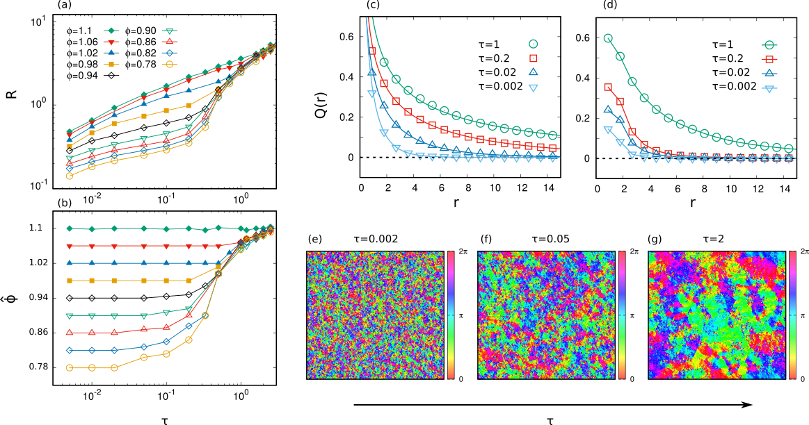
Figure 3: Size of the velocity aligned domains. In panels (a) and (b), we plot $R$ and $\phi$ as a function of $\tau$ for different values of ${\phi}$ as indicated in the caption. Panels (c) and (d) show the spatial correlations of the velocity orientation, $Q(r)$, for ${\phi}=1.1,0.94$, respectively. Curves with different $\tau$ are reported according to the caption. Panels (e), (f) and (g) show three different snapshot configurations for $\tau=0.002,0.05,2$, respectively, with $\phi=1.1$. All data in this figure are obtained at $v_{0}=50$.

Fig. 1 (c) and (d) are snapshots of the system representing particles’ positions and velocities for a large value of the persistence: they do not show MIPS, since at ${\phi}=1.1$ the density remains homogeneous in the considered range of $\tau$. In the case of interacting systems, the velocities of the particles, $\mathbf{v}_{i}$, represented by black arrows in Fig.1 (c)-(d), differ from $\mathbf{f}^{a}_{i}$ and, in spite of the absence of any alignment interactions, align and self-organize in large oriented domains. On the contrary, the self-propulsion $\mathbf{f}^{a}_{i}$ remains randomly oriented. The alignment of velocity orientations corresponds to the collective movements of large domains of particles. Such domains rearrange continuously in time and, sometimes, collapse into vortex structures, at variance with the well-known traveling bands occurring in the Vicsek-like models Grégoire and Chaté (2004); Chaté et al. (2008); Mishra et al. (2010); Menzel (2012).

Hereafter, such a velocity order is studied quantitatively in terms of spatial alignment velocity correlations and suitable order parameters, useful to estimate the size of the domains. We find that there are different aspects in the velocity ordering phenomenology: i) order in the orientation of the velocity vectors ii) order in the full velocity vectors, accounting also for the occurrence of large regions with the same kinetic energy.

III.1 Velocity orientation

For Vicsek-like models, the global alignment of the particles, also known as polarization, is commonly measured by the following order parameters Vicsek et al. (1995); Vicsek and Zafeiris (2012); Cavagna and Giardina (2014); Chaté et al. (2008):

$$\varphi=\frac{1}{N}\left|\sum_{i=1}^{N}e^{i\Theta_{k}}\right|\,,$$ (8)

where $i$ is the imaginary unit and $\Theta_{k}$ is the velocity orientation of the $k$-th particle. This observable is almost zero for particles without any alignment, typically at low numerical densities and high noise, and returns one, for perfectly aligned particles, e.g. for large values of $\phi$ Chaté et al. (2008). On the contrary in most systems of swimming active particles, typically evolved by means of overdamped equations, velocity vectors are ignored and the self-propulsion orientation is the only information used to characterize polarization: for instance, in the case of spherical (apolar) ABP particles, the parameter $\varphi$ in Eq. (8) - with $\Theta_{k}$ replaced by $\theta_{k}$ of Eq. (3) - is close to zero. In this model, since self-propulsions do not coincide with velocities, it is more suitable to consider the orientation of the velocity vector, $\dot{\mathbf{x}}_{k}$, in Eq. (8), i.e. replacing $\Theta_{k}$ with the angle formed by the velocity of the particle with respect to the $x$ axis. However, due to the presence of several domains with different orientations, there is no global velocity-polarization. In principle, for very large persistence we could observe a large oriented domain spanning the whole box, but such a finite size effect occurs only when $v_{0}\tau\gg L$, i.e. when the persistence length exceeds the size of the box Menzel and Löwen (2013); Menzel et al. (2014). We do not consider such a case in this manuscript.

A more appropriate indicator, which - even in the absence of a global polarization - gives information about the local alignment of the velocities and its dependence on physical parameters, is the spatial correlation function of the velocity-orientation, $Q_{i}(r)$ Caprini et al. (2020). This observable measures the velocity alignment between the particle $i$ and its neighboring particles located in the circular crown of thickness $\bar{r}=\sigma$ and mean radius $r=k\bar{r}$, being $k$ an integer positive number, and reads:

$$Q_{i}(r)=1-2\sum_{j}\frac{d_{ij}}{\mathcal{N}_{k}\pi}\,$$ (9)

where the sum runs over the particles within the circular crown defined by the value of $k$ and $\mathcal{N}_{k}$ corresponds to the number of particles contained in it. The term $d_{ij}$ is the angular distance between the two angles of the velocities of particles $i$ and $j$, namely $\beta_{i}$ and $\beta_{j}$, calculated as $d_{ij}=\text{min}\left[|\beta_{i}-\beta_{j}|,2\pi-|\beta_{i}-\beta_{j}|\right]$. We average over all particles by defining $Q(r)=\sum_{i}Q_{i}(r)/N$ which has the property of being $1$ and $-1$ for perfectly aligned and anti-aligned particles, respectively, and $0$ in the absence of any form of alignment. In panels (c-d) of Fig.3, we report $Q(r)$ for different values of the persistence time, $\tau$, and for two different densities. As expected $Q(r)$ is a decreasing function of $r$. For the smallest values of $\tau$, the alignment is appreciable only in the first shells, a finding consistent with the scenario where the self-propulsion only acts as an effective thermal diffusion. Instead, as $\tau$ increases, $Q(r)$ takes on larger values in the first shell and decays slower and slower towards zero, with a typical decay length which roughly represents the average size of one domain: larger values of $\tau$ and density (almost always) produce both the increasing of $Q(r)$ in the first shell ($k=1$) and the slower decay of the whole function. This observation is, also, qualitatively confirmed by three snapshot configurations obtained for increasing values of $\tau$ from panel (e) to panel (f) and (g) of Fig. 3. There, the colors encode the velocity orientations, showing the growth of the average size of the individual velocity domains with $\tau$.

The velocity ordering is well captured by the order parameter $R$, obtained by integrating over the whole box the correlation $Q(r)$:

$$R=\int Q(r)dr\,.$$ (10)

Such a parameter is a measure of the domain size and is studied in Fig. 3 (a), as $\tau$ varies for several values of $\phi$, evaluating both the homogeneous and the non-homogeneous configurations. We recall that the non-homogeneous regimes correspond to the emergence of empty regions or phase-separation, signaled by the presence of a non-single-peak in the packing fraction distribution (see Fig. 2 (d-e)). For the purpose of evaluating the impact of density inhomogeneity upon $R$, we show the main peak position, $\hat{\phi}$ in Fig. 3 (b), for different values of $\tau$ and average packing fraction $\phi$. We remark that $\hat{\phi}\approx\phi$ up to some critical value of $\tau$, then it increases. Such a critical value grows as the average packing $\phi$ is increased. At the larger packing fraction studied $\phi=1.1$ the system remains homogeneous for all the explored values of $\tau$. It is worthy to note that the values of $\hat{\phi}$ (the densities in the denser portion of the system) become independent from $\phi$ for $\tau$ sufficiently large.

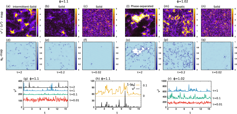
Figure 4: Fluctuations of kinetic energy. Panels (a)-(f) and (l)-(q) are snapshots in the plane $xy$ realized at $\phi=1.1,1.02$, respectively, for different values of $\tau$ as reported below the panels. Colors of panels (a), (b), (c) and (l), (m) and (n) encode the value of the square velocity of each particle, $v^{2}/\langle v^{2}\rangle$, while colors of panels (d), (e), (f) and (o), (p), (q) represent the value of the crystalline orientational order parameter $|\Psi_{6}|$. Panels (g) and (r) report different time-series of $v^{2}$ obtained for $\tau=10^{-2},10^{-1},1,2$ as indicated in the caption, with $\phi=1.1$ (panel (g)) and $\phi=1.02$ (panel (r)). Panel (h) compares a single trajectory of $v^{2}$ and $1-|\Psi_{6}|$, obtained with $\tau=2$ and $\phi=1.1$. All the simulations are realized with $v_{0}=50$.

As shown in panel (a), $R$ increases with $\tau$. For $\phi=1.1$, i.e. when the system is spatially homogeneous for all the values of $\tau$, the growth is steady. This proves that the growth of $R$ occurs even in the absence of any local density inhomogeneity since it is not associated with some local change of density. Instead, for smaller values of $\phi$, a first slow monotonic increase is followed by a sharp one occurring at a value of $\tau$ for which the homogeneous liquid-like or hexatic phases break down in favor of an inhomogeneous phase. The comparison between panels (a) and (b) also suggests that $R$ has a strong dependence on $\phi$.

The occurrence of such a velocity order is an evidence of the non-equilibrium nature of the dense active phases. Even if the structural (positional) information suggests an analogy with the liquid, hexatic or solid phases of a passive - equilibrium - system, there is not an equilibrium counterpart of the velocity ordering phenomenon.

In general, it is believed that the occurrence of local velocity alignment is a consequence of the breaking of some microscopic isotropy (as occurs in the case of rod or elongated particles Peruani et al. (2006); Ginelli et al. (2010); Abkenar et al. (2013); Peruani (2017)) or the introduction of explicit alignment interactions. The present ABP model subject to random independent active driving leads to velocities’ alignment - in the high-density regimes - even for spherical particles. This phenomenology simply arises from the interplay between self-propulsion and steric inter-particle repulsion.

III.2 Kinetic energy and intermittency

Besides the local order of velocity orientations, spatial correlations also manifest in the speed, $v=|\mathbf{v}|$, and, thus, in the kinetic energy of the particles, $\propto v^{2}$. Panels (a), (b) and (c) of Fig. 4 show the map of $v^{2}/\langle v^{2}\rangle$ for three snapshot configurations obtained varying $\tau$, for $\phi=1.1$, i.e. at a density value such that the active system attains a solid-like state for every $\tau$. For small $\tau$, kinetic energies display uncorrelated spatial fluctuations (with Gaussian statistics, not shown here). As $\tau$ grows, structures characterized by similar (or correlated) values of $v^{2}$ appear, with alternation of fast and slow regions (each identified by a given color).

We also highlight an interesting connection between the kinetic energy spatial distribution and the structural properties of the system. In panels (d), (e) and (f) of Fig. 4, we plot the observable $|\psi_{6}(\mathbf{x}_{i})|$ - which is the field pertaining to the crystalline orientational order - relative to the three configurations of panels (a), (b) and (c). The comparison between the maps of $|\psi_{6}(\mathbf{x}_{i})|$ and $v^{2}$ reveals that the regions with large kinetic energies develop close to the defects of the crystalline structure. A similar scenario occurs for a smaller value of $\phi$, namely $\phi=1.02$. In this case, the $v^{2}$-map is shown in panels (l), (m) and (n), while panels (o), (p) and (q) report the $|\psi_{6}|$-map. For this choice of $\phi$, the three values of $\tau$ distinguish between different aggregation phases: phase-separated, hexatic and solid (from the left to the right). The solid phase for the smaller value of $\tau$ is qualitatively indistinguishable from the denser case (compare the panels (c) and (n)). Instead, for the intermediate value of $\tau$ (panel m)) the occurrence of the hexatic phase is responsible for a larger number of defects and, thus, a larger number of mobile particles, as clearly shown from the comparison between panels (m) and (p). Finally, in the phase-separated configuration, the fastest regions are mostly concentrated near the boundary of the empty region (panel (l)).

To have another perspective, it is instructive to consider the time behavior of the kinetic energy, $v^{2}$, calculated averaging over a box of size $l$ such that $\bar{r}\ll L$. This observable, as a function of time, is reported for different values of $\tau$ in Fig. 4 (g) and (r) for $\phi=1.1,1.02$, respectively. In these two cases, the scenario is similar: for the smaller values of $\tau$ the kinetic energy displays symmetric and rapidly uncorrelated fluctuations around the mean value, $\langle v^{2}\rangle$. This is coherent with an effective equilibrium picture which is expected when $\tau\to 0$. For large values of $\tau$, sparse anomalous peaks manifest, corresponding to rare fluctuations, which move away from their average by several standard deviations. Such peaks become higher and more isolated when $\tau$ increases. The observed behavior resembles the temporal intermittency observed in turbulence Bohr et al. (2005). A more detailed analysis of such an issue will be presented in a future work, while, in this manuscript, we only consider the essential features of this phenomenon, in particular the role played by defects in the solid phase: particles near the defects attain - in fact - large kinetic energy. To corroborate our observation, we compare the fluctuations of the orientational order parameter, $\Psi_{6}=\sum_{i=1}^{N_{l}}\psi_{6,j}/N_{l}$, and those of kinetic energy, $v^{2}$, both averaged over a box of size $l$ with $N_{l}$ particles. In particular, Fig. 4 (h) shows the time-trajectories of $1-\Psi_{6}$ and $v^{2}$ revealing a fair correlation between the occurrence of spikes for both these observables.

With the aim of introducing also the information about intermittency in the general picture, we have drawn a dashed black line in the phase diagram of Fig. 1: the line identifies the intermittency region and is tracked at the first values of $\tau$ and $\phi$ for which the peaks of the $v^{2}$ trajectory overcomes $3$ times the standard deviation from its average value.

III.3 Vectorial velocity field

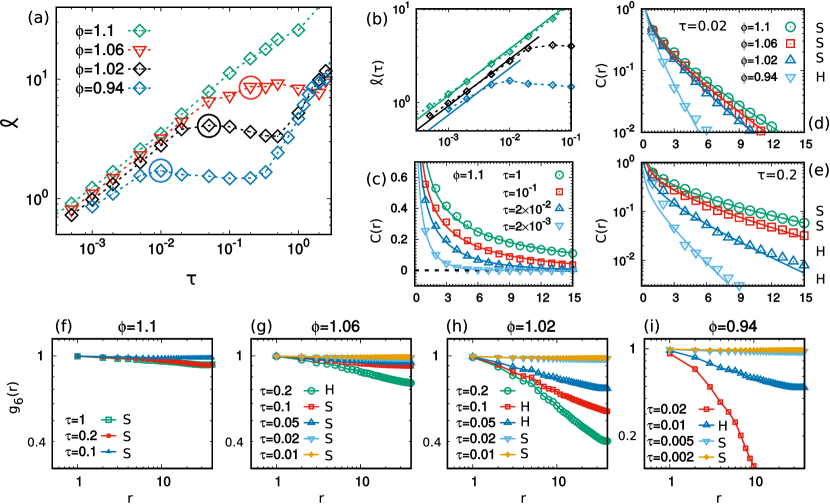
Figure 5: Spatial correlations of velocity vectors: theory and numerics. Panel (a) and (b) show the correlation lengths, $\ell$, as a function of $\tau$ for different values of $\phi$ as shown in the legend. The colored circle around a dot of each curve in panel (a) is the point at which the solid-hexatic transition is obtained. In particular, panel (b) zooms into small values of $\tau$ and shows the prediction (13) as a solid line, fitting the function $a\,\tau^{1/2}$, being $a$ a fitting parameter. Panels (c), (d) and (e) plot the correlation function $C(r)$ for several values of $\phi$ and $\tau$: for $\phi=1.1$ (i.e. in the solid- state) for several values of $\tau$ (panel (c)), and for two values of $\tau$ as a function of $\phi$ (panels (d) and (e) which share the same caption). In panels (c), (d), (e), points are obtained from numerical simulations while solid lines from the theoretical prediction, Eq. (12). The letters S and H near the curves mean “solid” and “hexatic” phase, respectively. Panels (f), (g), (h) and (i) report $g_{6}(r)$ for different values of $\phi$ and $\tau$. The simulations are realized with $v_{0}=50$.

In the previous Sections, we have seen that the spatial correlation of velocity orientations grows with $\tau$, even in the presence of crystalline defects or large voids (such as those in the phase-separated regimes). Speed (velocity modulus) is more sensitive to the presence of defects and creates patterns with sparse strong fluctuations. A natural question arises: what happens to the spatial correlation of the full velocity vectors (which incorporate both orientation and modulus)?

A quantitative measure of the ordering of the velocities can be obtained by measuring the spatial correlation function

$$C(r)=\frac{\langle\mathbf{v}(r)\cdot\mathbf{v}(0)\rangle}{\langle v^{2}\rangle}\,,$$ (11)

in the continuous limit, $\mathbf{v}_{i}\to\mathbf{v}(\mathbf{r})$. $\langle v^{2}\rangle$ is the variance of the velocity distribution calculated over the whole box. Our analysis limited to the case of homogeneous density under some assumptions is able to predict the form of $C(r)$ (as illustrated in Appendix B). The equation of motion (5) is approximated by the AOUP dynamics, replacing the multiplicative noise by a two-dimensional additive noise. By this method, it is possible to predict the spatial velocity correlation function. At variance with a similar calculation reported in Caprini et al. (2020), here we assume that particles are free to oscillate around their equilibrium positions, i.e. they form a hexagonal crystal structure with oscillating sites. Under these simple hypotheses, an expression for $C(r)$ can be derived using the equation of evolution of the velocities. In particular, $C(r)$ displays an exponential-like behavior:

$$C(r)\propto\frac{\bar{x}^{2}}{\ell^{2}}\Bigl{(}\frac{\ell}{8\pi r}\Bigr{)}^{1/2}e^{-r/\ell}\,,$$ (12)

where $\ell$ is the correlation length:

$$\ell=\bar{x}\sqrt{\frac{\tau}{\gamma}}\left[\frac{3}{4}\left(U^{\prime\prime}(\bar{r})+\frac{U^{\prime}(\bar{r})}{\bar{r}}\right)\right]^{1/2}\,.$$ (13)

Thus, a strong potential and/or a large value of $\tau$ increases the value of $\ell$. Also increasing the average packing fraction (i.e. decreasing the lattice constant $\bar{r}$) leads to a growth of $\ell$ through the $U(\bar{r})$ dependence on this quantity. Expression (13) coincides with the result obtained in Caprini et al. (2020), even if here it is derived under the less restrictive hypothesis of a vibrating (not rigid) lattice. Moreover, at variance with Caprini et al. (2020), here we are also considering very high average densities with homogeneous (not phase-separated) configurations, allowing us to directly check the scaling of $C(r)$ with $\tau$. On the contrary, when phase-separation occurs, the packing fraction $\hat{\phi}$ of the dense regions (and therefore the effective value of $\bar{r}$) grows with $\tau$, even at fixed average density $\phi$.

To check the predictions (12) and (13), we study the spatial velocity correlation, $C(r)$, for several values of $\tau$ and $\phi$. $C(r)$ for the denser case ($\phi=1.1$), which corresponds to the solid phase for the whole range of $\tau$ numerically explored, is reported in Fig. 5 (c) and reveals a good agreement with theory. The correlation length, $\ell$, is reported in Fig. 5 (a) (green diamonds) and shows a monotonic growth in fairly good agreement with Eq. (13): under these high-density conditions, the defects are not so statistically relevant and do not interfere with the velocity order. A zoom of Fig. 5, shown in panel (b) and accompanied by a fit of the numerical data, displays a good agreement with formula (13). A similar analysis reveals discrepancies between theory and simulations when applied to lower values of $\phi$: the growth of $\ell$ ceases at some value of $\tau$ which depends on $\phi$. We mark with a colored circle the first value of $\tau$ where $\ell$ has reached a plateau, and call it $\tau^{*}(\phi)$. Interestingly, this is close (up to numerical errors) to the value of $\tau$ where the solid-hexatic transition takes place (i.e. the fraction of crystalline defects roughly overcomes a given threshold), Here, for completeness, we report the correlation function of $\Psi_{6}$, namely $g_{6}=\langle\Psi_{6}(0)\Psi_{6}^{*}(r)\rangle$, in Fig. 5 (f)-(i). This function shows the well-known transition from the solid to the hexatic phases, roughly at $\tau^{*}$, where $g_{6}$ goes from a nearly constant behavior to a power-law decay Cugliandolo and Gonnella (2018). For comparison, we also show $C(r)$ as a function of $\phi$ for two different values of $\tau$, in panels (d) and (e), where each phase is signed by S, H (solid, hexatic) in the caption. In the hexatic phase, $C(r)$ maintains the exponential-like shape predicted in Eq. (12) but decays abruptly much faster in the proximity of the solid-hexatic transition. As a consequence, the agreement between Eq. (13) and data, shown in Fig. 5 (b), holds up to $\tau^{*}$, while for $\tau>\tau^{*}$ the presence of defects invalidates the prediction (13) since $\ell$ remains nearly constant or decay very slowly. It is also remarkable that a further increase of $\tau$ produces a steep growth of $\ell$. This is likely caused by phase-separation and the increase of local density in the clustered regions. Even in this case, we still expect that Eq. (13) holds even if the function $\bar{x}(\tau)$ is unknown.

In conclusion, we have solid arguments to state that a large number of defects, occurring in the hexatic or liquid phase, is responsible for the saturation of $\ell$. Indeed, in the proximity of a defect, regions with large kinetic energies are present, as seen in the previous section, and, as a consequence, the velocities are less correlated. Interestingly, the size $R$ of the orientational domains is not so affected by the lack of orientational order, always revealing a monotonic growth with $\tau$ independently of the structural phase.

IV Discussion and perspectives

We have studied systems of self-propelled particles at high packing fractions displaying structural properties which resemble the equilibrium liquid, hexatic and solid phases, exploring both the small and the large persistence regime.

While at small values of the persistence time, $\tau$, many observables behave as in equilibrium, the phenomenology in the high persistence regime is much richer and displays unexpected phenomena. We conclude that an improved active phase diagram benefits from the introduction of new order parameters, related to velocity correlations which have not a Brownian counterpart.

In particular, velocities exhibit intriguing patterns, forming aligned domains or vortex-like arrangements. We propose a suitable order parameter which quantifies the size of these domains, deduced from the spatial correlations of the velocity orientations. Such a parameter grows with both packing fraction, $\phi$, and $\tau$ in the homogeneous phases, but it becomes independent from $\phi$ in the phase-separated regimes. We also observe the occurrence of large regions whose kinetic energy is highly correlated: these regions become larger when $\tau$ and $\phi$ grow. Besides, high energetic regions form in the proximity of orientational defects of the solid phase, much more visible in the hexatic phase where defects are diffuse. This is accompanied by a pronounced time intermittency phenomenon, apparently well-correlated to the fluctuations of the orientational order parameter. Correlations of the full velocity vector are also useful to get insights about these dynamical features, in particular, they can be successfully compared to a mesoscopic theory developed under the assumption of homogeneous density. Deviations from the theory appear together with the emergence of a large fraction of defects and the breakdown of homogeneity.

Our observations call for experimental verifications. Promising real platforms to confirm such interesting phenomenologies are Janus particles Takatori et al. (2016); Klongvessa et al. (2019) or vibrated polar granular disks Briand and Dauchot (2016).

In the present work, we have been interested in understanding the dense phase in monodisperse active systems. Binary mixtures are often employed for gaining insight into active glass phases Berthier and Biroli (2011); Berthier et al. (2019); Janssen (2019); Szamel et al. (2015); Berthier et al. (2017, 2019); Ni et al. (2013); Mandal et al. (2016); Nandi et al. (2018). In particular, it has been shown that the spatial velocity correlation function is an input ingredient for developing a self-consistent Mode-Coupling Theory of Active Matter Szamel et al. (2015). Our findings prove that, as a general result, the statistical properties of the velocity field have to be taken into account for providing a complete description of active systems. As a future direction, it would be interesting to understand how the velocity alignment patterns we observed modify glassy transition.

The phenomenology of domains with aligned velocities could resemble the scenario of traveling crystals, observed in Refs. Menzel and Löwen (2013); Menzel et al. (2014) in numerical simulations. Recently, traveling crystals have been observed in experiments using suspensions of micro-disks subjected to vertical vibrations Briand et al. (2018). In such studies, the whole hexagonal pattern moves coherently in space, even though each self-propulsion vector points randomly. Our phenomenology is quite different since far particles (which belong to different domains) move independently and, thus, the whole crystal gets stuck. Instead, the movement of some clusters gives rise to the formation of defects. We find that the whole crystal travels coherently as in Ref. Menzel and Löwen (2013) only if the size of the box is smaller than the persistence length of the active motion.

Acknowledgements

LC thanks M. Cencini and A. Cavagna for fruitful discussions. AP and MP acknowledge funding from Regione Lazio, Grant Prot. n. 85-2017-15257 (”Progetti di Gruppi di Ricerca - Legge 13/2008 - art. 4”). LC, UMBM, and AP acknowledge support from the MIUR PRIN 2017 project 201798CZLJ.

Appendix A Velocity dynamics in the case $T>0$

The change of variables from $(\mathbf{x}_{i},\mathbf{f}^{a}_{i})$ to $(\mathbf{x}_{i},\mathbf{v}_{i})$, i.e. from Eqs. (1) and (3) to Eqs. (4) and (5), has been derived in Ref. Caprini et al. (2020) in the absence of thermal noise (i.e. for $T=0$). The change of variables can be easily generalized to the case $T>0$, as shown in this Appendix. Such a generalization follows the strategy of Ref. Caprini and Marconi (2018), where the result is obtained in the case of the AOUP model for non-interacting particles. Here, the same trick can be adapted to the ABP self-propulsion. To overcome the difficulty regarding the time-derivation of the thermal noise, we define the variable $\mathbf{v}_{i}=\dot{\mathbf{x}}_{i}-\sqrt{2T/\gamma}\,\bm{w}_{i}$. Taking the derivative with respect to the time, the dynamics reads:

$$\dot{\mathbf{x}}_{i} =\mathbf{v}_{i}+\sqrt{2T/\gamma}\,\bm{w}_{i}$$ (14)

$$\tau\gamma\dot{\mathbf{v}}_{i} =-\gamma\sum_{j=1}^{N}{\Gamma}_{ij}({\mathbf{r}}_{ij})\mathbf{v}_{j}+\mathbf{F}_{i}+\tau\gamma\mathbf{k}_{i}$$ (15)

$$\qquad\qquad\qquad-\tau\nabla_{i}\cdot\mathbf{F}_{i}\sqrt{2T/\gamma}\bm{w}_{i}\,.$$

The thermal noise comes into play with two additional noise terms. The first is an additive noise on the dynamics of $\dot{\mathbf{x}}_{i}$, while the second is multiplicative and acts on $\dot{\mathbf{v}}_{i}$. Its space prefactor balances the space-dependent Stokes force in the equilibrium limit $\tau\to 0$.

Appendix B Positional, orientational and velocity correlations for a perfect active lattice

In order to obtain the correlation functions of the two-dimensional system we shall make two simplifying assumptions in the dynamics, Eq. (1):

• each component of the active force, $\mathbf{f}^{a}_{i}$, is replaced by independent Ornstein-Uhlenbeck processes, namely $\bm{\eta}_{i}$, with equivalent intensity, $v_{0}=\sqrt{D/\tau}$ and persistence time, $1/D_{r}=\tau$;

• each particle oscillates around a node of a hexagonal lattice so that the total inter-particle potential can be approximated as the sum of quadratic terms.

The approximate dynamics reads:

$$\dot{\bm{\eta}}_{i}(t)=-\frac{1}{\tau}\bm{\eta}_{i}(t)+\frac{\sqrt{2D}}{\tau}\bm{\xi}_{i}(t)$$ (16)

$$\dot{\bf x}_{i}(t)=\bm{\eta}_{i}(t)-\sum_{j}^{n.n}\frac{\nabla_{i}U(|{\bf x}_{j}-{\bf x}_{i}|)}{\gamma}\,,$$ (17)

where $\nabla_{i}U$ stands for the gradient of the potential $U$ with respect to ${\bf x}_{i}$ and the sum involves the nearest neighbors of the lattice node $i$.

Introducing the displacement ${\bf u}_{i}$ of the particle $i$ with respect to its equilibrium position, ${\bf x}^{0}_{i}$, namely

$${\bf u}_{i}={\bf x}_{i}-{\bf x}^{0}_{i}\,,$$ (18)

we get

$$\dot{\bm{\eta}}_{i}(t)=-\frac{1}{\tau}\bm{\eta}_{i}(t)+\frac{\sqrt{2D}}{\tau}\bm{\xi}_{i}(t)$$ (19)

$$\dot{\bf u}_{i}(t)=\bm{\eta}_{i}(t)+\frac{K}{\gamma}\sum_{\bf m}^{n.n}({\bf u}_{j}-{\bf u}_{i})\,,$$ (20)

where $K$ is the strength of the potential in the harmonic approximation, i.e. $U\approx\frac{K}{2}({\bf u}_{j}-{\bf u}_{i})^{2}$, which reads

$$2K=\left(U^{\prime\prime}(a)+\frac{U^{\prime}(a)}{a}\right)\,,$$

being $a=\bar{x}$ the lattice constant. In order to solve the problem, we switch to normal coordinates, employing the Fourier space representation:

$$\hat{\bf u}_{{\bf q}}=\frac{1}{N}\sum_{i}{\bf u}_{i}\,e^{-i{\bf q}\cdot{\bf x}^{0}_{i}}$$ (21)

$$\hat{\bm{\eta}}_{{\bf q}}=\frac{1}{N}\sum_{i}\bm{\eta}_{i}\,e^{-i{\bf q}\cdot{\bf x}^{0}_{i}}\,,$$ (22)

and obtain

$$\frac{d}{dt}\hat{\bm{\eta}}_{\bf q}(t)=-\frac{1}{\tau}\hat{\bm{\eta}}_{\bf q}+\frac{\sqrt{2D}}{\tau}\hat{\bm{\xi}}_{\bf q}$$ (23)

$$\frac{d}{dt}\hat{\bf u}_{\bf q}(t)=-\frac{\omega^{2}_{\bf q}}{\gamma}\hat{\bf u}_{\bf q}(t)+\hat{\bm{\eta}}_{\bf q}\,,$$ (24)

where

$$\omega_{\bf q}^{2} =-2K\Bigl{[}\cos(q_{x}a)+2\cos\Bigl{(}\frac{1}{2}q_{x}a\Bigr{)}\cos\Bigl{(}\frac{\sqrt{3}}{2}q_{y}a\Bigr{)}-3\Bigr{]}$$

$$\approx\frac{3}{2}Ka^{2}q^{2}+O(q^{4})\,,$$ (25)

where $\mathbf{q}=(q_{x},q_{y})$ are vectors of the reciprocal Bravais lattice. Thus, we can easily calculate the steady-state equal time correlations:

$$\langle\hat{{\bf u}}_{\bf q}(t)\cdot\hat{{\bf u}}_{-{\bf q}}(t)\rangle=\frac{2D\gamma}{\omega_{\bf q}^{2}\left(1+\frac{\tau}{\gamma}\omega_{\bf q}^{2}\right)}$$ (26)

$$\langle\hat{{\bf v}}_{\bf q}(t)\cdot\hat{{\bf v}}_{-{\bf q}}(t)\rangle=\frac{2D}{\tau}\frac{1}{1+\frac{\tau}{\gamma}\omega_{\bf q}^{2}}$$ (27)

$$\langle\hat{{\bf u}}_{\bf q}(t)\cdot\hat{{\bf v}}_{-{\bf q}}(t)\rangle=0$$ (28)

B.1 Velocity correlation function

We, now, consider the real-space velocity correlation function:

$$\langle{\bf v}_{\bf x}\cdot{\bf v}_{\bf x^{\prime}}\rangle=\frac{1}{N^{2}}\frac{2D}{\tau}\sum_{{\bf q}}e^{i{\bf q}({\bf x}-{\bf x}^{\prime})}\frac{1}{(1+\frac{\tau}{\gamma}\omega_{\bf q}^{2})}\,.$$ (29)

By replacing the lattice sum by a double dimensional integral and defining $r=|{\bf x}-{\bf x^{\prime}}|$, we have

$$\langle{\bf v}_{\bf x}\cdot{\bf v}_{\bf x^{\prime}}\rangle\approx\frac{1}{2\pi}\frac{2D}{\tau}\frac{a^{2}}{\ell^{2}}K_{0}(r/\ell)$$ (30)

where $K_{0}(r/\ell)$ is the zero-order modified Bessel function of the second kind which has the following asymptotic behavior when $r/\ell\gg 1$:

$$K_{0}(r/\ell)\approx\Bigl{(}\frac{\pi\ell}{2r}\Bigr{)}^{1/2}e^{-r/\ell}\,,$$

we find

$$\langle{\bf v}_{\bf x}\cdot{\bf v}_{\bf x^{\prime}}\rangle\approx 2v_{0}^{2}\frac{a^{2}}{\ell^{2}}\Bigl{(}\frac{\ell}{8\pi r}\Bigr{)}^{1/2}e^{-r/\ell}\,,$$ (31)

where

$$\ell^{2}=\frac{3\tau}{2\gamma}a^{2}K=\frac{3\tau}{4\gamma}a^{2}\Bigl{(}U^{\prime\prime}(a)+\frac{U^{\prime}(a)}{a}\Bigr{)}\,,$$

which defines the correlation length $\ell$ in the harmonic hexagonal lattice in agreement with the result (13).

B.2 Bond angle order and $\psi_{6}$-field in the harmonic crystal

We define the angle, $\alpha_{{\bf x}}$, between the local crystallographic axes and the axes of the ideal lattice Brock (1992):

$$\alpha_{{\bf x}}=\frac{1}{2}\nabla\times{\bf u}_{{\bf x}}\,.$$

where we used the continuum representation. In Fourier space we have:

$$\hat{\alpha}_{{\bf q}}=\frac{i}{2}(q_{x}\hat{u}_{{\bf q}y}-q_{y}\hat{u}_{{\bf q}x})$$

while the $\hat{\alpha}_{{\bf q}}$ correlation reads

$$\langle\hat{\alpha}_{{\bf q}}\hat{\alpha}_{-{\bf q}}\rangle=\frac{D\gamma}{4}\frac{q^{2}}{\omega_{\bf q}^{2}}\frac{1}{1+\frac{\tau}{\gamma}\omega_{\bf q}^{2}}\approx\frac{\sigma^{2}}{6a^{2}}\frac{1}{1+\ell^{2}q^{2}}\,,$$

where $\sigma^{2}=D\gamma/K$. The real-space $\alpha_{\mathbf{x}}$-correlation function is given by

$$\langle(\alpha_{{\bf x}}-\alpha_{{\bf x}^{\prime}})^{2}\rangle \propto\frac{1}{N^{2}}\sum_{{\bf q}}e^{i{\bf q}({\bf x}-{\bf x}^{\prime})}\frac{\sigma^{2}}{6a^{2}}\frac{1}{1+\ell^{2}q^{2}}$$

$$\propto\Bigl{(}\frac{\ell}{8\pi r}\Bigr{)}^{1/2}\frac{a^{2}}{\ell^{2}}e^{-r/\ell}\,.$$

where we have used the expansion for small $\mathbf{q}$ and the asymptotic behavior of $K_{0}(r/l)$. Now, we consider the correlation function of $\psi_{6{{\bf x}}}=e^{i6\alpha_{{\bf x}}}$

$$\langle\psi_{6{{\bf x}}}\psi^{*}_{6{{\bf x}^{\prime}}}\rangle=\langle e^{i6\alpha_{{\bf x}}}e^{-i6\alpha_{{\bf x}^{\prime}}}\rangle\,.$$

Using the form of the $\alpha$-correlation we find:

$$\langle\psi_{6{\bf x}}\psi^{*}_{6{\bf x}^{\prime}}\rangle=e^{-\frac{1}{2}\langle(6\alpha_{{\bf x}}-6\alpha_{{\bf x}^{\prime}})^{2}\rangle}\,.$$

Consequently, the correlator of $\psi_{6}$ does not vanishes at infinity, i.e. the order is maintained since:

$$\lim_{|{\bf x}-{\bf x}^{\prime}|\to\infty}\langle\psi_{6{\bf x}}\psi^{*}_{6{\bf x}^{\prime}}\rangle=const\,.$$

This is the expected result since the harmonic lattice always maintains the sixfold coordination number and no disclinations can be created. We notice that for this model the velocity correlation and the $\alpha_{{\bf x}}$-correlation have the same long-range behavior.

References

- Löwen (1994) H. Löwen, Physics Reports 237, 249 (1994).
- Gasser (2009) U. Gasser, Journal of Physics: Condensed Matter 21, 203101 (2009).
- Mermin and Wagner (1966) N. D. Mermin and H. Wagner, Physical Review Letters 17, 1133 (1966).
- Mermin (1968) N. D. Mermin, Physical Review 176, 250 (1968).
- Halperin and Nelson (1978) B. I. Halperin and D. R. Nelson, Phys. Rev. Lett. 41, 121 (1978).
- Young (1979) A. P. Young, Phys. Rev. B 19, 1855 (1979).
- Berezinsky (1970) V. Berezinsky, Zh. Eksp. Teor. Fiz. 32, 493 (1970).
- Kosterlitz and Thouless (1973) J. M. Kosterlitz and D. J. Thouless, Journal of Physics C: Solid State Physics 6, 1181 (1973).
- Gasser et al. (2010) U. Gasser, C. Eisenmann, G. Maret, and P. Keim, ChemPhysChem 11, 963 (2010).
- Zahn et al. (1999) K. Zahn, R. Lenke, and G. Maret, Physical Review Letters 82, 2721 (1999).
- Dullens et al. (2017) R. Dullens, A. Thorneywork, J. Abbott, and D. Aarts, Physical Review Letters 118 (2017).
- Marchetti et al. (2013) M. Marchetti, J. Joanny, S. Ramaswamy, T. Liverpool, J. Prost, M. Rao, and R. A. Simha, Reviews of Modern Physics 85, 1143 (2013).
- Gompper et al. (2020) G. Gompper, R. G. Winkler, T. Speck, A. Solon, C. Nardini, F. Peruani, H. Löwen, R. Golestanian, U. B. Kaupp, L. Alvarez, et al., Journal of Physics: Condensed Matter 32, 193001 (2020).
- Bechinger et al. (2016) C. Bechinger, R. Di Leonardo, H. Löwen, C. Reichhardt, G. Volpe, and G. Volpe, Reviews of Modern Physics 88, 045006 (2016).
- Klongvessa et al. (2019) N. Klongvessa, F. Ginot, C. Ybert, C. Cottin-Bizonne, and M. Leocmach, arXiv preprint arXiv:1902.01746 (2019).
- Deseigne et al. (2010) J. Deseigne, O. Dauchot, and H. Chaté, Physical Review Letters 105, 098001 (2010).
- Briand and Dauchot (2016) G. Briand and O. Dauchot, Physical Review Letters 117, 098004 (2016).
- Angelini et al. (2011) T. E. Angelini, E. Hannezo, X. Trepat, M. Marquez, J. J. Fredberg, and D. A. Weitz, Proceedings of the National Academy of Sciences 108, 4714 (2011).
- Garcia et al. (2015) S. Garcia, E. Hannezo, J. Elgeti, J.-F. Joanny, P. Silberzan, and N. S. Gov, Proceedings of the National Academy of Sciences 112, 15314 (2015).
- Mongera et al. (2018) A. Mongera, P. Rowghanian, H. J. Gustafson, E. Shelton, D. A. Kealhofer, E. K. Carn, F. Serwane, A. A. Lucio, J. Giammona, and O. Campàs, Nature 561, 401 (2018).
- Bialké et al. (2012) J. Bialké, T. Speck, and H. Löwen, Physical Review Letters 108, 168301 (2012).
- Menzel and Löwen (2013) A. M. Menzel and H. Löwen, Physical Review Letters 110, 055702 (2013).
- Menzel et al. (2014) A. M. Menzel, T. Ohta, and H. Löwen, Physical Review E 89, 022301 (2014).
- Briand et al. (2018) G. Briand, M. Schindler, and O. Dauchot, Physical Review Letters 120, 208001 (2018).
- Digregorio et al. (2018) P. Digregorio, D. Levis, A. Suma, L. F. Cugliandolo, G. Gonnella, and I. Pagonabarraga, Physical Review Letters 121, 098003 (2018).
- Cugliandolo et al. (2017) L. F. Cugliandolo, P. Digregorio, G. Gonnella, and A. Suma, Physical Review Letters 119, 268002 (2017).
- Stenhammar et al. (2014) J. Stenhammar, D. Marenduzzo, R. J. Allen, and M. E. Cates, Soft Matter 10, 1489 (2014).
- Klamser et al. (2018) J. U. Klamser, S. C. Kapfer, and W. Krauth, Nature Communications 9, 5045 (2018).
- Redner et al. (2013) G. S. Redner, M. F. Hagan, and A. Baskaran, Physical Review Letters 110, 055701 (2013).
- Buttinoni et al. (2013) I. Buttinoni, J. Bialké, F. Kümmel, H. Löwen, C. Bechinger, and T. Speck, Physical Review Letters 110, 238301 (2013).
- Palacci et al. (2013) J. Palacci, S. Sacanna, A. P. Steinberg, D. J. Pine, and P. M. Chaikin, Science 339, 936 (2013).
- Bialké et al. (2015a) J. Bialké, T. Speck, and H. Löwen, Journal of Non-Crystalline Solids 407, 367 (2015a).
- Ginot et al. (2018) F. Ginot, I. Theurkauff, F. Detcheverry, C. Ybert, and C. Cottin-Bizonne, Nature Communications 9, 696 (2018).
- Siebert et al. (2017) J. T. Siebert, J. Letz, T. Speck, and P. Virnau, Soft Matter 13, 1020 (2017).
- Speck (2016) T. Speck, The European Physical Journal Special Topics 225, 2287 (2016).
- Chiarantoni et al. (2020) P. Chiarantoni, F. Cagnetta, F. Corberi, G. Gonnella, and A. Suma, arXiv preprint arXiv:2001.08500 (2020).
- Fily and Marchetti (2012) Y. Fily and M. C. Marchetti, Physical Review Letters 108, 235702 (2012).
- Cates and Tailleur (2015) M. E. Cates and J. Tailleur, Annual Review of Condensed Matter Physics 6, 219 (2015).
- Gonnella et al. (2015) G. Gonnella, D. Marenduzzo, A. Suma, and A. Tiribocchi, Comptes Rendus Physique 16, 316 (2015).
- Ma et al. (2020) Z. Ma, M. Yang, and R. Ni, arXiv preprint arXiv:2004.02376 (2020).
- Solon et al. (2015a) A. P. Solon, Y. Fily, A. Baskaran, M. E. Cates, Y. Kafri, M. Kardar, and J. Tailleur, Nature Physics 11, 673 (2015a).
- Solon et al. (2015b) A. P. Solon, J. Stenhammar, R. Wittkowski, M. Kardar, Y. Kafri, M. E. Cates, and J. Tailleur, Physical Review Letters 114, 198301 (2015b).
- Bialké et al. (2015b) J. Bialké, J. T. Siebert, H. Löwen, and T. Speck, Physical Review Letters 115, 098301 (2015b).
- Patch et al. (2018) A. Patch, D. M. Sussman, D. Yllanes, and M. C. Marchetti, Soft Matter 14, 7435 (2018).
- Mandal et al. (2019) S. Mandal, B. Liebchen, and H. Löwen, Physical Review Letters 123, 228001 (2019).
- Caprini et al. (2020) L. Caprini, U. M. B. Marconi, and A. Puglisi, Physical Review Letters 124, 078001 (2020).
- Puglisi et al. (2012) A. Puglisi, A. Gnoli, G. Gradenigo, A. Sarracino, and D. Villamaina, J. Chem. Phys. 014704, 136 (2012).
- Manacorda (2018) A. Manacorda, Lattice Models for Fluctuating Hydrodynamics in Granular and Active Matter (Springer, 2018).
- Plati et al. (2019) A. Plati, A. Baldassarri, A. Gnoli, G. Gradenigo, and A. Puglisi, Phys. Rev. Lett. 123, 038002 (2019).
- Farage et al. (2015) T. F. Farage, P. Krinninger, and J. M. Brader, Physical Review E 91, 042310 (2015).
- Vicsek and Zafeiris (2012) T. Vicsek and A. Zafeiris, Physics Reports 517, 71 (2012).
- Grégoire and Chaté (2004) G. Grégoire and H. Chaté, Physical Review Letters 92, 025702 (2004).
- Lam et al. (2015) K.-D. N. T. Lam, M. Schindler, and O. Dauchot, New Journal of Physics 17, 113056 (2015).
- Giavazzi et al. (2018) F. Giavazzi, M. Paoluzzi, M. Macchi, D. Bi, G. Scita, M. L. Manning, R. Cerbino, and M. C. Marchetti, Soft matter 14, 3471 (2018).
- Caprini and Marconi (2018) L. Caprini and U. M. B. Marconi, Soft Matter 14, 9044 (2018).
- Marconi and Maggi (2015) U. M. B. Marconi and C. Maggi, Soft Matter 11, 8768 (2015).
- Marconi et al. (2017) U. M. B. Marconi, A. Puglisi, and C. Maggi, Scientific Reports 7, 46496 (2017).
- Marconi et al. (2016) U. M. B. Marconi, N. Gnan, M. Paoluzzi, C. Maggi, and R. Di Leonardo, Scientific Reports 6, 23297 (2016).
- Fodor et al. (2016) É. Fodor, C. Nardini, M. E. Cates, J. Tailleur, P. Visco, and F. van Wijland, Physical Review Letters 117, 038103 (2016).
- Wittmann et al. (2019) R. Wittmann, F. Smallenburg, and J. M. Brader, The Journal of chemical physics 150, 174908 (2019).
- Berthier et al. (2019) L. Berthier, E. Flenner, and G. Szamel, The Journal of Chemical Physics 150, 200901 (2019).
- Caprini et al. (2019a) L. Caprini, U. M. B. Marconi, A. Puglisi, and A. Vulpiani, Journal of Statistical Mechanics: Theory and Experiment 2019, 053203 (2019a).
- Woillez et al. (2019) E. Woillez, Y. Kafri, and V. Lecomte, arXiv preprint arXiv:1912.04010 (2019).
- Caprini and Marconi (2019) L. Caprini and U. M. B. Marconi, Soft Matter 15, 2627 (2019).
- Maggi et al. (2017) C. Maggi, M. Paoluzzi, L. Angelani, and R. Di Leonardo, Scientific Reports 7, 17588 (2017).
- Caprini et al. (2019b) L. Caprini, E. Hernández-García, C. López, and U. M. B. Marconi, Scientific reports 9, 1 (2019b).
- Das et al. (2018) S. Das, G. Gompper, and R. G. Winkler, New Journal of Physics 20, 015001 (2018).
- Caprini et al. (2019c) L. Caprini, U. M. B. Marconi, and A. Puglisi, Scientific Reports 9, 1386 (2019c).
- Cugliandolo and Gonnella (2018) L. F. Cugliandolo and G. Gonnella, arXiv preprint arXiv:1810.11833 (2018).
- Chaté et al. (2008) H. Chaté, F. Ginelli, G. Grégoire, and F. Raynaud, Physical Review E 77, 046113 (2008).
- Mishra et al. (2010) S. Mishra, A. Baskaran, and M. C. Marchetti, Physical Review E 81, 061916 (2010).
- Menzel (2012) A. M. Menzel, Physical Review E 85, 021912 (2012).
- Vicsek et al. (1995) T. Vicsek, A. Czirók, E. Ben-Jacob, I. Cohen, and O. Shochet, Physical Review Letters 75, 1226 (1995).
- Cavagna and Giardina (2014) A. Cavagna and I. Giardina, Annu. Rev. Condens. Matter Phys. 5, 183 (2014).
- Peruani et al. (2006) F. Peruani, A. Deutsch, and M. Bär, Physical Review E 74, 030904 (2006).
- Ginelli et al. (2010) F. Ginelli, F. Peruani, M. Bär, and H. Chaté, Physical review letters 104, 184502 (2010).
- Abkenar et al. (2013) M. Abkenar, K. Marx, T. Auth, and G. Gompper, Physical Review E 88, 062314 (2013).
- Peruani (2017) F. Peruani, Journal of the Physical Society of Japan 86, 101010 (2017).
- Bohr et al. (2005) T. Bohr, M. H. Jensen, G. Paladin, and A. Vulpiani, Dynamical systems approach to turbulence (Cambridge University Press, 2005).
- Takatori et al. (2016) S. C. Takatori, R. De Dier, J. Vermant, and J. F. Brady, Nature Communications 7, 10694 (2016).
- Berthier and Biroli (2011) L. Berthier and G. Biroli, Reviews of Modern Physics 83, 587 (2011).
- Janssen (2019) L. Janssen, arXiv preprint arXiv:1906.03678 (2019).
- Szamel et al. (2015) G. Szamel, E. Flenner, and L. Berthier, Physical Review E 91, 062304 (2015).
- Berthier et al. (2017) L. Berthier, E. Flenner, and G. Szamel, New Journal of Physics 19, 125006 (2017).
- Ni et al. (2013) R. Ni, M. A. C. Stuart, and M. Dijkstra, Nature Communications 4, 2704 (2013).
- Mandal et al. (2016) R. Mandal, P. J. Bhuyan, M. Rao, and C. Dasgupta, Soft Matter 12, 6268 (2016).
- Nandi et al. (2018) S. K. Nandi, R. Mandal, P. J. Bhuyan, C. Dasgupta, M. Rao, and N. S. Gov, Proceedings of the National Academy of Sciences 115, 7688 (2018).
- Brock (1992) J. D. Brock, in Bond-orientational order in condensed matter systems (Springer, 1992) pp. 1–31.