An Averaging Processes on Hypergraphs

Abstract

Consider the following iterated process on a hypergraph $H$. Each vertex $v$ starts with some initial weight $x_{v}$. At each step, uniformly at random select an edge $e$ in $H$, and for each vertex $v$ in $e$ replace the weight of $v$ by the average value of the vertex weights over all vertices in $e$. This is a generalization of an interactive process on graphs which was first introduced by Aldous and Lanoue. In this paper we use the eigenvalues of a Laplacian for hypergraphs to bound the rate of convergence for this iterated averaging process.

1 Introduction

The following iterated process on a graph $G$ was introduced by Aldous and Lanoue [2].

Initially, assign $n$ real numbers $x_{1},\ldots,x_{n}$ to the vertices of $G$. At each step uniformly at random select $\{i,j\}\in E(G)$ and replace both $x_{i}$ and $x_{j}$ with their average value $(x_{i}+x_{j})/2$.

As noted in [2], this process was motivated by the study of social dynamics and interactive particle systems. Recently Chaterjee, Diaconis, Sly, and Zhang [6] further investigated this process in response to a question of Bourgain and a problem arising in quantum computing. In particular they obtained sharper estimates for the rate of convergence for the case of $G$ being a complete graph.

There are various procedures similar to the above process, such as the gossip algorithms studied by Shah [15], the distributed consensus algorithms studied by Olshevsky and Tsitsiklis [13], and various restricted averaging processes [1, 3] as well as numerous ‘smoothing’ or ‘renewal’ models in statistics [7, 10]. In addition, there are numerous random processes sharing similar flavors and methods, such as exchanging processes on permutations and card shuffling [9].

In this paper, we consider the following averaging process on a hypergraph $H$, and we emphasize that we place no restriction on the multiplicity or size of any edge of $H$.

Initially, assign $n$ real numbers $x_{1},\ldots,x_{n}$ to the vertices of $H$. At each step uniformly at random select an edge $e\in E(H)$, and for each $i\in e$ replace $x_{i}$ with the average value $|e|^{-1}\sum_{j\in e}x_{j}$.

Let us formalize this process somewhat. Recall that a hypergraph $H$ is a set of vertices $V(H)$ together with a multiset $E(H)$ of subsets of $V(H)$ which are called edges. Given a hypergraph $H$, let $x$ be a real-valued vector indexed by $V(H)$, which we call a weight vector of $H$. Define the (random) vector $\mathbf{\mathrm{R}}_{H}(x)$ by choosing an edge $e$ uniformly at random from $E(H)$, and then setting $\mathbf{\mathrm{R}}_{H}(x)_{u}=x_{u}$ if $u\notin e$ and $\mathbf{\mathrm{R}}_{H}(x)_{u}=|e|^{-1}\sum_{v\in e}x_{v}$ otherwise. Recursively define $\mathbf{\mathrm{R}}_{H}^{t}(x)=\mathbf{\mathrm{R}}_{H}(\mathbf{\mathrm{R}}_{H}^{t-1}(x))$. Equivalently, $\mathbf{\mathrm{R}}_{H}^{t}(x)$ is the random vector obtained by uniformly generating a sequence of $t$ edges and then performing the averaging process for each edge sequentially. When $H$ is understood we simply write $\mathbf{\mathrm{R}}^{t}(x)$.

Given a weight vector $x$ of $H$ with $|V(H)|=n$, define the vector $\overline{x}=(\frac{1}{n}\sum x_{u},\ldots,\frac{1}{n}\sum x_{u})$. We wish to determine how quickly $\mathbf{\mathrm{R}}^{t}(x)$ converges to $\overline{x}$ in various norms. In the graph setting, Aldous and Lanoue [2] bounded this rate of convergence in terms of the second smallest eigenvalue of the (combinatorial) Laplacian. There are many ways to generalize the Laplacian for hypergraphs [8, 11, 12], and in this paper we use a generalization which was introduced by Rodríguez [14].

Given a hypergraph $H$, the codegree $d(u,v)$ of two vertices $u\neq v$ is defined to be the number of edges $e$ containing both $u$ and $v$ in $H$. If $H$ is an $n$-vertex hypergraph, the codegree Laplacian $L(H)$ is the $n\times n$ matrix with $L(H)_{u,v}=-d(u,v)$ if $u\neq v$ and $L(H)_{u,u}=\sum_{v\neq u}d(u,v)$. For example, if $n=4$ and $E(H^{\prime})=\{\{1,2\},\{1,2\},\{2,3,4\}\}$, then

$$L(H^{\prime})=\begin{bmatrix}2&-2&0&0\\ -2&4&-1&-1\\ 0&-1&2&-1\\ 0&-1&-1&2\end{bmatrix}.$$

Note that when $H$ is a graph this reduces to the Laplacian matrix of $H$. In fact, $L(H)$ can be defined to be the Laplacian for the multi-graph $G_{H}$ obtained by placing a clique on all of the vertices of each $e\in E(H)$. For example, with $H^{\prime}$ as above, $G_{H^{\prime}}$ is the multi-graph displayed below.

1.1 Main Results

It is clear that $L(H)$ is a real symmetric matrix, and hence it has $n$ real eigenvalues which we denote by $\lambda_{0}(H)\leq\lambda_{1}(H)\leq\cdots\leq\lambda_{n-1}(H)$. With this in mind we can state our main result.

Theorem 1.1.

Let $H$ be a hypergraph with $|e|\geq r$ for all $e\in E(H)$. Then for all weight vectors $x$ and $t\geq 1$,

$$\mathbb{E}\left[\lVert\mathbf{\mathrm{R}}^{t}(x)-\overline{x}\rVert_{2}^{2}\right]\leq\left(1-\frac{\lambda_{1}(H)}{r|E(H)|}\right)^{t}\lVert x-\overline{x}\rVert_{2}^{2}.$$

With this we will bound the rate of convergence for connected hypergraphs. We recall that a hypergraph $H$ is connected if for every non-empty subset $S\subsetneq V(H)$ there exists an edge $e\in E(H)$ containing a vertex in $S$ and $V(H)\setminus S$.

Corollary 1.2.

Let $H$ be a connected hypergraph on $n$ vertices such that $|e|\geq r$ for all $e\in E(H)$. For all weight vectors $x$, the iterated averaging process converges to its average value $\bar{x}$ as follows:

$$\mathbb{E}\left[\lVert\mathbf{\mathrm{R}}^{t}(x)-\overline{x}\rVert_{2}\right]\leq e^{-c}\lVert x-\overline{x}\rVert_{2} \textrm{ whenever }t\geq 2c\cdot\frac{r|E(H)|}{\lambda_{1}(H)},$$

$$\mathbb{E}\left[\lVert\mathbf{\mathrm{R}}^{t}(x)-\overline{x}\rVert_{1}\right]\leq e^{-c}\lVert x-\overline{x}\rVert_{2} \textrm{ whenever }t\geq(\log(n)+2c)\cdot\frac{r|E(H)|}{\lambda_{1}(H)}.$$

Chaterjee, Diaconis, Sly, and Zhang [6] showed that these bounds are essentially tight when $H$ is the complete graph $K_{n}$.

One can obtain concentration results for certain hypergraphs. To this end, a hypergraph $H$ is said to be codegree regular if there exists some $d$ with $d(u,v)=d$ for all $u\neq v$. Examples of codegree regular hypergraphs include $K_{n}^{(r)}$ (the hypergraph on $\{1,\ldots,n\}$ with edge set consisting of every set of size $r$) and Steiner systems (hypergraphs where every pair is covered by exactly one edge). Also recall that $H$ is $r$-uniform if $|e|=r$ for all $e\in E(H)$.

Theorem 1.3.

Let $H$ be an $n$-vertex $r$-uniform hypergraph which is codegree regular. Then for all weight vectors $x$ and $t\geq 1$,

$$\mathbb{E}\left[\lVert\mathbf{\mathrm{R}}^{t}(x)-\overline{x}\rVert_{2}^{2}\right]=\left(1-\frac{r-1}{n-1}\right)^{t}\lVert x-\overline{x}\rVert_{2}^{2}.$$ (1)

Moreover, $\lim\lVert\mathbf{\mathrm{R}}^{t}(x)-\overline{x}\rVert_{2}^{2}/\left(1-\frac{r-1}{n-1}\right)^{t}$ exists and is finite almost surely.

The conclusions of Theorem 1.3 do not hold in general if $H$ is not codegree regular, see Propositions 4.1 and 4.2.

Lastly, we note that the hypergraph averaging process can be used to model other averaging processes for which our results also apply. In particular, we define the neighborhood averaging process as follows. Let $G$ be a simple graph and define the neighborhood $N_{G}(u)$ of a vertex $u\in V(G)$ to be the set of vertices adjacent to $u$ in $G$. For $x$ a weight vector of $G$, define the weight vector $\mathbf{\tilde{\mathrm{R}}}_{G}(x)$ by uniformly at random selecting some $u\in V(G)$, and then setting $\mathbf{\tilde{\mathrm{R}}}_{G}(x)_{v}=x_{v}$ if $v\notin N_{G}(u)$ and $\mathbf{\tilde{\mathrm{R}}}_{G}(x)_{v}=\frac{1}{|N_{G}(u)|}\sum_{w\in N_{G}(u)}x_{w}$ otherwise. We iteratively define $\mathbf{\tilde{\mathrm{R}}}_{G}^{t}(x)=\mathbf{\tilde{\mathrm{R}}}_{G}(\mathbf{\tilde{\mathrm{R}}}_{G}^{t-1}(x))$ and denote this simply by $\mathbf{\tilde{\mathrm{R}}}^{t}(x)$ whenever $G$ is understood.

Theorem 1.4.

Let $G$ be an $n$-vertex $d$-regular graph and define $\lambda^{\prime}:=\min\{\lambda_{1}(G),2d-\lambda_{n-1}(G)\}$. Then for all weight vectors $x$ and $t\geq 1$,

$$\mathbb{E}\left[\lVert\mathbf{\tilde{\mathrm{R}}}^{t}(x)-\overline{x}\rVert_{2}^{2}\right]\leq\left(1-\frac{\lambda^{\prime}(2d-\lambda^{\prime})}{dn}\right)^{t}\lVert x-\overline{x}\rVert_{2}^{2}.$$

From this one can obtain bounds analogous to those of Corollary 1.2 whenever $G$ is connected and not bipartite.

The rest of the paper is organized as follows. In Section 2 we prove some basic facts about the codegree Laplacian $L(H)$. We then prove Theorems 1.1 and 1.4 in Section 3 along with Corollary 1.2. In Section 4 we prove Theorem 1.3 and provide some counterexamples to concentration. We close the paper with a number of open problems in Section 5.

2 Preliminaries

In this section we state and prove several basic results about $L(H)$, all of which are easy generalizations of the analogous results for graphs. To start, we show that the Raleigh quotient of $L(H)$ has a particularly nice form. To simplify our lemmas, we adopt the convention that $\sum_{u,v}$ denotes the sums over all unordered pairs $\{u,v\}$ with $u\neq v$.

Lemma 2.1.

For $x\neq 0$ a real vector,

$$\frac{x^{T}L(H)x}{x^{T}x}=\frac{\sum_{u,v}d(u,v)(x_{u}-x_{v})^{2}}{\lVert x\rVert_{2}^{2}}$$

Proof.

The denominator is clear. For the numerator, by definition we have

$$(L(H)x)_{u}=\sum_{v\neq u}d(u,v)x_{u}-\sum_{v\neq u}d(u,v)x_{v}=\sum_{v\neq u}d(u,v)(x_{u}-x_{v}).$$

Thus

$$x^{T}L(H)x=\sum_{u}\sum_{v\neq u}d(u,v)(x_{u}^{2}-x_{u}x_{v})$$

$$=\sum_{u,v}d(u,v)(x_{u}^{2}+x_{v}^{2}-2x_{u}x_{v})=\sum_{u,v}d(u,v)(x_{u}-x_{v})^{2}.$$

∎

We recall the following well known linear algebra results, which can be found, for example, in [4].

Lemma 2.2 ([4]).

Let $M$ be a real $n\times n$ symmetric matrix. Then $M$ has $n$ real eigenvalues $\lambda_{0}\leq\cdots\leq\lambda_{n-1}$ and

$$\lambda_{0}=\min_{0\neq x\in\mathbb{R}^{n}}\frac{x^{T}Mx}{x^{T}x}.$$

Further, any $x_{0}$ achieving this equality is an eigenvector corresponding to $\lambda_{0}$ and

$$\lambda_{1}=\min_{0\neq x\in\mathbb{R}^{n}:x\perp x_{0}}\frac{x^{T}Mx}{x^{T}x}.$$

Putting these lemmas together gives the following.

Lemma 2.3.

For all hypergraphs $H$, $\lambda_{0}(H)=0$ and

$$\lambda_{1}(H)=\min_{0\neq x\in\mathbb{R}^{n}:\sum x_{v}=0}\frac{\sum_{u,v}d(u,v)(x_{u}-x_{v})^{2}}{\lVert x\rVert_{2}^{2}}.$$

Moreover, $\lambda_{1}(H)>0$ if and only if $H$ is connected.

Proof.

Because $L(H)$ is real symmetric, we have from Lemmas 2.2 and 2.1 that $\lambda_{0}(H)$ is the minimum over non-zero real $x$ of

$$\frac{\sum_{u,v}d(u,v)(x_{u}-x_{v})^{2}}{\lVert x\rVert_{2}^{2}}$$ (2)

Because the numerator and denominator of (2) are sums of squares, $\lambda_{0}(H)\geq 0$. Moreover, by taking $x=(1,\ldots,1)$ we see that the minimum is exactly 0 and that the all 1’s vector is a corresponding eigenvector. By Lemma 2.2, $\lambda_{1}(H)$ is the minimum of (2) subject to $x\perp(1,\ldots,1)$, i.e. subject to $\sum x_{u}=0$. From this it follows that $\lambda_{1}(H)=0$ if and only if there exists a non-zero $x$ with $\sum d(u,v)(x_{u}-x_{v})^{2}=0$ and $\sum x_{u}=0$, and we claim this happens if and only if $H$ is disconnected.

Indeed, if $H$ has a subset $S\subseteq V(H)$ such that every edge contains only vertices in $S$ or $V(H)\setminus S$, then we can take the vector $x$ with $x_{u}=|S|^{-1}$ if $u\in S$ and $x_{u}=-|V(H)\setminus S|^{-1}$ if $u\notin S$; and one can verify that $x$ satisfies the conditions above, proving that $\lambda_{1}(H)=0$. Conversely, if such an $x$ exists, let $S_{1}=\{u\in V(H):x_{u}\geq 0\}$ and $S_{2}=\{u\in V(H):x_{u}<0\}$. Because $x\neq 0$ and $\sum x_{u}=0$ these two sets are non-empty, and hence both are proper subsets of $V(H)$. Moreover, there exists no edge $e\in E(H)$ with $u,v\in e$, $u\in S_{1}$, and $v\in S_{2}$, as this would imply $d(u,v)(x_{u}-x_{v})^{2}>0$. Thus $S_{1}\subsetneq V(H)$ shows that $H$ is disconnected as desired. ∎

3 Bounding the Rate of Convergence

It turns out that one can express how much $\lVert\mathbf{\mathrm{R}}(x)\rVert_{2}^{2}$ differs from $\lVert x\rVert_{2}^{2}$ in a concise form.

Lemma 3.1.

For any weight vector $x$ with $\sum x_{u}=0$,

$$\mathbb{E}\left[\lVert x\rVert_{2}^{2}-\lVert\mathbf{\mathrm{R}}(x)\rVert_{2}^{2}\right]=\frac{1}{|E(H)|}\sum_{e\in E(H)}\frac{1}{|e|}\sum_{u,v\in e}(x_{u}-x_{v})^{2}.$$

Proof.

Assume the edge $e$ is chosen in the averaging process. Then

$$\lVert x\rVert_{2}^{2}-\lVert\mathbf{\mathrm{R}}(x)\rVert_{2}^{2}=\left(\sum_{u\in e}x_{u}^{2}\right)-|e|\left(\frac{\sum_{v\in e}x_{v}}{|e|}\right)^{2}$$

$$=\frac{1}{|e|}\left(\sum_{u\in e}(|e|-1)x_{u}^{2}-2\sum_{u,v\in e}x_{u}x_{v}\right)=\frac{1}{|e|}\sum_{u,v\in e}(x_{u}-x_{v})^{2}.$$

As each edge is equally likely to be chosen, we conclude the result. ∎

With this we can prove our main theorem.

Proof of Theorem 1.1.

Let $x^{\prime}$ be a weight vector. It is not difficult to see that $\mathbf{\mathrm{R}}^{t}(x^{\prime})-\overline{x}^{\prime}=\mathbf{\mathrm{R}}^{t}(x^{\prime}-\overline{x}^{\prime})$. Thus it is enough to prove the result for $x:=x^{\prime}-\overline{x^{\prime}}$, and with this we have $\sum x_{u}=0$ and $\overline{x}=0$.

By Lemma 3.1 and the bound $|e|\geq r$,

$$\mathbb{E}[\lVert x\rVert_{2}^{2}-\lVert\mathbf{\mathrm{R}}(x)\rVert_{2}^{2}]=\frac{1}{|E(H)|}\sum_{e\in E(H)}\frac{1}{|e|}\sum_{u,v\in e}(x_{u}-x_{v})^{2}$$

$$\geq\frac{1}{r|E(H)|}\sum_{e\in E(H)}\sum_{u,v\in e}(x_{u}-x_{v})^{2}=\frac{1}{r|E(H)|}\sum_{u,v}d(u,v)(x_{u}-x_{v})^{2}.$$

By Lemma 2.3 this quantity is at most $\frac{1}{r|E(H)|}\lambda_{1}(H)\lVert x\rVert_{2}^{2}$. By removing the determinstic value $\lVert x\rVert_{2}^{2}$ out of the expectation, we see that the result holds for $t=1$, and the result in general follows by inductively applying the $t=1$ bound. ∎

Proof of Corollary 1.2.

For the first result, we use the inequality $\mathbb{E}[X]\leq\sqrt{\mathbb{E}[X^{2}]}$, Theorem 1.1, and the inequality $1-\tau\leq e^{-\tau}$ to conclude that

$$\mathbb{E}\left[\lVert\mathbf{\mathrm{R}}^{t}(x)-\overline{x}\rVert_{2}\right] \leq\sqrt{\mathbb{E}[\lVert\mathbf{\mathrm{R}}^{t}(x)-\overline{x}\rVert_{2}^{2}]}$$

$$\leq\left(1-\frac{\lambda_{1}(H)}{r|E(H)|}\right)^{t/2}\lVert x-\overline{x}\rVert_{2}\leq\exp\left(\frac{-t\lambda_{1}(H)}{2r|E(H)|}\right)\lVert x-\overline{x}\rVert_{2}.$$

Plugging in $t=2c\cdot\frac{r|E(H)|}{\lambda_{1}(H)}$ gives the result, and we note that Lemma 2.3 and $H$ connected implies $\lambda_{1}(H)\neq 0$ so this is well defined.

For the second result, we use the Cauchy-Schwarz inequality and Theorem 1.1 to deduce that

$$\mathbb{E}\left[\lVert\mathbf{\mathrm{R}}^{t}(x)-\overline{x}\rVert_{1}\right] \leq\sqrt{\mathbb{E}\left[n\cdot\lVert\mathbf{\mathrm{R}}^{t}(x)-\overline{x}\rVert_{2}^{2}\right]}$$

$$\leq\sqrt{n}\left(1-\frac{\lambda_{1}(H)}{e(G)r}\right)^{t/2}\lVert x-\overline{x}\rVert_{2}\leq\exp\left(\frac{1}{2}\log(n)-\frac{t\lambda_{1}(H)}{2r|E(H)|}\right)\lVert x-\overline{x}\rVert_{2}.$$

Plugging in $t=(\log(n)+2c)\cdot\frac{r|E(H)|}{\lambda_{1}(H)}$ gives the result. ∎

We recall that a walk of length $k$ in a graph $G$ is a sequence of (possibly not distinct) vertices $v_{0},v_{1},\ldots,v_{k}$ such that $v_{i}\sim v_{i+1}$ for all $0\leq i<k$. The following standard result can be found in [4].

Lemma 3.2 ([4]).

Let $A(G)$ be the adjacency matrix of a graph. Then $A^{k}(G)_{u,v}$ is the number of walks of length $k$ from $u$ to $v$.

Proof of Theorem 1.4.

Given a simple graph $G$, we define an auxiliary hypergraph $H_{G}$ by $V(H_{G})=V(G)$ and $E(H_{G})=\{N_{G}(u):u\in V(G)\}$. Observe that $H_{G}$ has $n$ edges each of size $d$. It is not difficult to see that $\mathbf{\tilde{\mathrm{R}}}_{G}^{t}(x)$ and $\mathbf{\mathrm{R}}_{H_{G}}^{t}(x)$ have the same distribution, so by Theorem 1.1 we have

$$\mathbb{E}[\lVert\mathbf{\tilde{\mathrm{R}}}_{G}^{t}(x)-\overline{x}\rVert_{2}^{2}]=\mathbb{E}[\lVert\mathbf{\mathrm{R}}_{H_{G}}^{t}(x)-\overline{x}\rVert_{2}^{2}]\leq\left(1-\frac{\lambda_{1}(H_{G})}{dn}\right)^{t}\lVert x-\overline{x}\rVert_{2}^{2}.$$ (3)

Note that for $u\neq v$, the codegree $d(u,v)$ in $H_{G}$ is equal to the number of common neighbors of $u$ and $v$ in $G$, which is exactly the number of walks of length 2 from $u$ to $v$ in $G$. Thus by Lemma 3.2 we have $L(H_{G})_{u,v}=-A^{2}(G)_{u,v}$ for $u\neq v$ and

$$L(H_{G})_{u,u}=\sum_{v\neq u}A^{2}(G)_{u,v}=d^{2}-A^{2}(G)_{u,u},$$

where this last step used that there are $d^{2}$ total walks of length 2 starting from $u$. We conclude that $L(H_{G})=d^{2}I-A^{2}(G)$. Because $G$ is $d$-regular, $A(G)=dI-L(G)$, and in particular the eigenvalues of $A^{2}(G)$ are exactly $(d-\lambda_{i}(G))^{2}$. Thus the eigenvalues of $L(H_{G})$ will be

$$d^{2}-(d-\lambda_{i}(G))^{2}=\lambda_{i}(G)(2d-\lambda_{i}(G)).$$

The smallest eigenvalue of $L(H_{G})$ will be $0$ corresponding to $i=0$, and the second smallest eigenvalue will be

$$\min\{\lambda_{1}(G)(2d-\lambda_{1}(G)),\lambda_{n-1}(G)(2d-\lambda_{n-1}(G))\}=\lambda^{\prime}(2d-\lambda^{\prime}),$$

and this together with (3) gives the result. ∎

4 Concentration Results

Proof of Theorem 1.3.

For ease of notation we assume $\overline{x}=0$, which we can do by the same argument used in the proof of Theorem 1.1. Assume $d(u,v)=d$ for all $u\neq v$. In this case $L(H)=dnI-dJ$ where $J$ is the all 1’s matrix. Thus the all 1’s vector together with the $n-1$ vectors $(1,0,\ldots,0,-1,0,\ldots,0)$ form an orthogonal space of eigenvectors for $L(H)$, with the latter eigenvectors all corresponding to the eigenvalue $dn$. In particular, every vector with $\sum x_{u}=0$ is an eigenvector corresponding to the eigenvalue $dn$. Using this and Lemmas 3.1 and 2.1 gives that for all $x$ with $\sum x_{u}=0$,

$$\mathbb{E}[\lVert x\rVert_{2}^{2}-\lVert\mathbf{\mathrm{R}}(x)\rVert_{2}^{2}] =\frac{1}{r|E(H)|}\sum_{u\neq v}d(u,v)(x_{u}-x_{v})^{2}$$

$$=\frac{1}{r|E(H)|}\cdot x^{T}L(H)x=\frac{nd}{r|E(H)|}\lVert x\rVert_{2}^{2}.$$

Pulling out the deterministic value $\lVert x\rVert_{2}^{2}$ gives

$$\mathbb{E}[\lVert\mathbf{\mathrm{R}}(x)\rVert_{2}^{2}]=\left(1-\frac{nd}{r|E(H)|}\right)\lVert x\rVert_{2}^{2}.$$

To complete the proof of (1) when $t=1$, we must show that $|E(H)|=\frac{n(n-1)d}{r(r-1)}$. To do this, we count the pairs $(\{u,v\},e)$ with $u\neq v$ and $u,v\in e$ in two ways. We can first choose the pair $\{u,v\}$ in ${n\choose 2}$ ways and then the edge in $d$ ways, or we could choose the edge first in $|E(H)|$ ways and then a pair it contains in ${r\choose 2}$ ways. This implies that ${n\choose 2}d=|E(H)|{r\choose 2}$, giving the desired result. The result for general $t$ follows by inductively applying the $t=1$ case.

For the concentration result, define $S^{t}(x)=(1-\frac{r-1}{n-1})^{-t}\cdot\mathbf{\mathrm{R}}^{t}(x)$, which in particular implies $S^{t}(x)=(1-\frac{r-1}{n-1})^{-1}\cdot\mathbf{\mathrm{R}}(S^{t-1}(x))$. This together with (1) implies that given $S^{t-1}(x)$, we have

$$\mathbb{E}\left[\lVert S^{t}(x)\rVert_{2}^{2}\right]=\frac{\mathbb{E}\left[\lVert\mathbf{\mathrm{R}}(S^{t-1}(x))\rVert_{2}^{2}\right]}{(1-\frac{r-1}{n-1})}=\lVert S^{t-1}(x)\rVert_{2}^{2}.$$

Thus $\lVert S^{t}(x)\rVert_{2}^{2}$ is a non-negative martingale, so its limit exists and is finite almost surely. ∎

We close this section with some examples where $H$ is not codegree regular and where the conclusions of Theorem 1.3 fail to hold. Here and throughout when we consider weight vectors $x$ on the path graph $P_{n}$, we let $x_{1},x_{n}$ be the weights of the endpoints of the path.

Proposition 4.1.

Let $x$ be the weight vector of $P_{3}$ with $x=(1,-\frac{1}{2},-\frac{1}{2})$. Then for all $t\geq 1$,

$$\Pr\left[\lVert\mathbf{\mathrm{R}}^{t}(x)\rVert_{2}^{2}\geq 2^{-t/2}\right]\geq\frac{1}{2}.$$

In contrast, Theorem 1.3 would predict that $\mathbb{E}[\lVert\mathbf{\mathrm{R}}^{t}(x)\rVert_{2}^{2}](2-\epsilon)^{t}$ tends to 0 for all $\epsilon>0$ if $P_{3}$ were codegree regular.

Proof.

Let $D(t)$ denote the number of $s$ with $1\leq s\leq t$ such that $\mathbf{\mathrm{R}}^{s}(x)\neq\mathbf{\mathrm{R}}^{s-1}(x)$. One can prove by induction that if $D(t)$ is even then $\mathbf{\mathrm{R}}^{t}(x)=(2^{-D(t)},-2^{-D(t)-1},-2^{-D(t)-1})$ and otherwise $\mathbf{\mathrm{R}}^{t}(x)=(2^{-D(t)-1},2^{-D(t)-1},-2^{-D(t)})$. In particular, given $D(t)$ we have $\lVert\mathbf{\mathrm{R}}^{t}(x)\rVert_{2}^{2}\geq 2^{-D(t)}$. Thus it is enough to show that $\Pr[D(t)\leq t/2]\geq\frac{1}{2}$. It is not difficult to see that the distribution of $D(t)$ is binomial with $t$ trials and probability $\frac{1}{2}$ of successes (each round has probability $\frac{1}{2}$ of choosing the one edge that will change $\mathbf{\mathrm{R}}^{t}(x)$). Thus this statement is equivalent to showing that $\sum_{i=0}^{t/2}{t\choose i}\geq 2^{t-1}$, which is easy to prove by the symmetry of the binomial coefficients. ∎

A similar example shows that there exist $x$ such that $\mathbf{\mathrm{R}}^{t}(x)$ can exhibit different long term behaviors.

Proposition 4.2.

Let $x$ be the weight vector of $P_{3}$ with $x=(1,-1,0)$. Then for all $t\geq 1$,

$$\Pr\left[\lVert\mathbf{\mathrm{R}}^{t}(x)\rVert_{2}^{2}=0\right]=\frac{1}{2},$$

$$\Pr\left[\lVert\mathbf{\mathrm{R}}^{t}(x)\rVert_{2}^{2}\geq 2^{-t}\right]=\frac{1}{2}.$$

Proof.

Let $x=(1,-1,0)$. With probability $\frac{1}{2}$ the edge $\{1,2\}$ is chosen first, and then for all $t\geq 1$ we have $\mathbf{\mathrm{R}}^{t}(x)=0$. If $\{2,3\}$ is chosen first then $\mathbf{\mathrm{R}}^{1}(x)=(1,-\frac{1}{2},-\frac{1}{2})$. In this case, the same reasoning as in the previous proof shows that $\lVert\mathbf{\mathrm{R}}^{t+1}(x)\rVert_{2}^{2}\geq 2^{-D(t)}$ with $D(t)$ a random variable that is at most $t$ (we shift $t$ by 1 here because this is the second step of this random process). In particular, we have $\lVert\mathbf{\mathrm{R}}^{t}(x)\rVert_{2}^{2}\geq 2^{-t}$ for all $t$ in this case. ∎

5 Concluding Remarks

For ease of presentation, whenever $H$ is understood we define

$$\Delta_{1}(t,x)=\lVert\mathbf{\mathrm{R}}_{H}^{t}(x)-\overline{x}\rVert_{1}.$$

The second half of Corollary 1.2 shows that in expectation $\Delta_{1}(t,x)$ will be small provided $t\approx\frac{r|E(H)|\log(n)}{\lambda_{1}(H)}$, and this bound is essentially tight for the complete graph $K_{n}$ due to work of Chaterjee, Diaconis, Sly, and Zhang [6]. It is not clear whether these bounds are tight for all hypergraphs, or even for all graphs, and we ask the following somewhat vague question.

Question 5.1.

When are the bounds in Corollary 1.2 essentially tight?

We give two concrete conjectures in this direction. Let $S_{n}$ be the star graph on $n+1$ vertices. Note that $|E(S_{n})|=n$ and $\lambda_{1}(G)=1$, so Corollary 1.2 shows that for any $x$ we have $\Delta_{1}(t,x)\approx 0$ in expectation whenever $t\approx 2n\log(n)$. We suspect that this is tight.

Conjecture 5.2.

Let $x$ be the weight vector on $S_{n}$ which gives weight $1-\frac{1}{n+1}$ to the central vertex and weight $-\frac{1}{n+1}$ to every other vertex. Then for $t=o(n\log n)$ we have

$$\mathbb{E}[\Delta_{1}(t,x)]\sim\lVert x-\overline{x}\rVert_{2}$$

Figure 1 shows a plot of $\Delta_{1}(t,x)$ for this $x$ and $S_{1000}$. Note that in this case $2n\log(n)\approx 13,800$, and it does appear to take this long for $\Delta_{1}(t,x)$ to converge to 0.

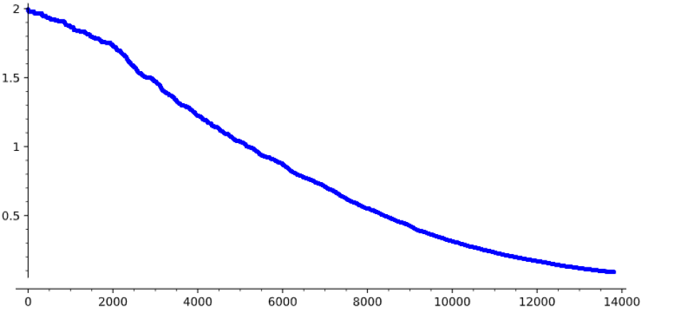
Figure 1: $\Delta_{1}(t,x)$ for $S_{1000}$ with $x_{1}=1-\frac{1}{1001}$ and $x_{i}=\frac{-1}{1001}$ for all other $i$.

On the other hand, we do not expect the bound of Corollary 1.2 to be tight for paths. If $P_{n}$ is the path graph on $n$ vertices, then $\lambda_{1}(P_{n})=2-2\cos(\pi/n)=\Theta(n^{-2})$ and Corollary 1.2 implies that $\Delta_{1}(t,x)$ will be small for $t=\Theta(n^{3}\log(n))$. Figure 2 gives a plot of $\Delta_{1}(t,x)$ when $x$ is the weight vector of $P_{40}$ taking value $\pm 1$ on each endpoint of the path and 0 everywhere else; and Figure 3 shows a plot when $x$ has weight $1-1/40$ on one endpoint and $-1/40$ on every vertex. Note that both processes seem to converge within $n^{3}=64,000$ steps. These results motivate us to conjecture that the $\log(n)$ term in Corollary 1.2 is not necessary for the path.

Figure 2: $\Delta_{1}(t,x)$ for $P_{40}$ with $x_{1}=1,\ x_{40}=-1$ and $0$ elsewhere.

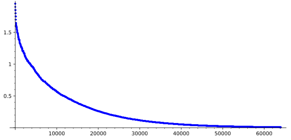
Figure 3: $\Delta_{1}(t,x)$ for $P_{40}$ with $x_{1}=1-\frac{1}{40}$ and $x_{i}=\frac{-1}{40}$ for all other $i$.

Conjecture 5.3.

For all $c>0$, there exists a constant $M=M(c)$ such that for all weight vectors $x$ of $P_{n}$, we have

$$\mathbb{E}[\Delta_{1}(Mn^{3},x)]\leq e^{-c}\lVert x-\overline{x}\rVert_{2}.$$

We now turn our attention to the neighborhood averaging process. By adapting the proof of Theorem 1.4 one can obtain bounds on the convergence of $\mathbf{\tilde{\mathrm{R}}}_{G}^{t}(x)$ for all graphs $G$ in terms of $\lambda_{1}(H_{G})$, where $H_{G}$ is the auxiliary hypergraph introduced in the proof of Theorem 1.4; and more precisely one can show that $\mathbf{\tilde{\mathrm{R}}}_{G}^{t}(x)$ will always converge to $\overline{x}$ if and only if $G$ is connected and not bipartite.

Unfortunately, it is impossible to express $\lambda_{1}(H_{G})$ in terms of $\lambda_{i}(G)$ for general graphs $G$. Indeed, it is well known that the eigenvalues of the Laplacian $L(G)$ can not detect whether $G$ is bipartite in general, so in particular it can not detect whether $\mathbf{\tilde{\mathrm{R}}}_{G}^{t}(x)$ will always converge to $\overline{x}$. However, it may be possible to express $\lambda_{1}(H_{G})$ in terms of eigenvalues of a different matrix associated to $G$. The most natural candidate would be the normalized Laplacian $\mathcal{L}(G)$ since its eigenvalues can detect whether $G$ is connected and bipartite in general; see the survey of Butler and Chung [5] for more on the normalized Laplacian. With this in mind we pose the following question.

Question 5.4.

For any connected and not bipartite graph $G$, can one bound the convergence of $\mathbf{\tilde{\mathrm{R}}}_{G}^{t}(x)$ in terms of the eigenvalues of the normalized Laplacian matrix $\mathcal{L}(G)$?

References

• [1] D.ย AcemoฤŸlu, G.ย Como, F.ย Fagnani, and A.ย Ozdaglar. Opinion fluctuations and disagreement in social networks. Mathematics of Operations Research, 38(1):1โ€“27, 2013.
• [2] D.ย Aldous, D.ย Lanoue, etย al. A lecture on the averaging process. Probability Surveys, 9:90โ€“102, 2012.
• [3] E.ย Ben-Naim, P.ย L. Krapivsky, and S.ย Redner. Bifurcations and patterns in compromise processes. Physica D: nonlinear phenomena, 183(3-4):190โ€“204, 2003.
• [4] A.ย E. Brouwer and W.ย H. Haemers. Spectra of graphs. Springer Science & Business Media, 2011.
• [5] S.ย Butler and F.ย Chung. Spectral graph theory. Handbook of linear algebra, pageย 47, 2006.
• [6] S.ย Chatterjee, P.ย Diaconis, A.ย Sly, and L.ย Zhang. A phase transition for repeated averages. arXiv preprint arXiv:1911.02756, 2020.
• [7] S.ย Chatterjee and E.ย Seneta. Towards consensus: Some convergence theorems on repeated averaging. Journal of Applied Probability, pages 89โ€“97, 1977.
• [8] F.ย Chung. The laplacian of a hypergraph. Expanding graphs (DIMACS series), pages 21โ€“36, 1993.
• [9] P.ย Diaconis and L.ย Saloff-Coste. Comparison techniques for random walk on finite groups. The Annals of Probability, pages 2131โ€“2156, 1993.
• [10] W.ย Feller. An introduction to probability theory and its applications, vol 2. John Wiley & Sons, 2008.
• [11] K.ย Feng etย al. Spectra of hypergraphs and applications. Journal of number theory, 60(1):1โ€“22, 1996.
• [12] L.ย Lu and X.ย Peng. High-ordered random walks and generalized laplacians on hypergraphs. In International Workshop on Algorithms and Models for the Web-Graph, pages 14โ€“25. Springer, 2011.
• [13] A.ย Olshevsky and J.ย N. Tsitsiklis. Convergence speed in distributed consensus and averaging. SIAM Journal on Control and Optimization, 48(1):33โ€“55, 2009.
• [14] J.ย A. Rodrรญguez. On the laplacian eigenvalues and metric parameters of hypergraphs. Linear and Multilinear Algebra, 50(1):1โ€“14, 2002.
• [15] D.ย Shah. Gossip algorithms (foundations and trends in networking), 2007.