Pomeron-LQCD model of $J/\Psi$ photo-production on the nucleon

Abstract

Based on the vector meson dominance assumption, a Hamiltonian model has been developed to investigate $J/\Psi$ photo-production reaction on the nucleon by using the $J/\Psi$-nucleon potential extracted from a lattice QCD calculation of Phys. Rev. D82, 091501 (2010). It is found that the predicted total cross sections are comparable to the recent data of $J/\Psi$ photo-production reaction from Jefferson Laboratory. The model is then extended to include the two-gluon exchange amplitude modeled by Donnachie and Lanshoff within Regge Phenomenology. The resulting Pomeron-LQCD model can then explain the data up to invariant mass $W=$ 300 GeV. Future improvements needed to reduce the uncertainties of the predictions are discussed. The need of an accurate extraction of $J/\Psi$-N potential at short distances from LQCD is illustrated.

I Introduction

The $J/\Psi$-nucleon ($N$) interaction is mediated by gluon exchanges within Quantum Chromodynamics (QCD). It has been investigated by using lattice QCD (LQCD) and the data of the extracted $J/\Psi$-N potential $v_{LQCD}(r)$ have been published by Kawanai and Sasakisasaki ; sasaki-1 . The purpose of this work is to explore how this LQCD potential can be used to predict $J/\Psi$ photo-production reaction cross sections, and how it can be combined with the Pomeron-exchange model, as developed in Refs.dl ; ohlee ; wulee , to explain the recent datajlab from Jefferson Laboratory (JLab) and also the earlier data up to invariant mass $W=300$ GeV.

In section II, we review the Pomeron-exchange model formulated in Refs.ohlee ; wulee . A model based on the vector meson dominance (VMD) and the LQCD potential $v_{LQCD}(r)$ is presented in section III. In section IV, the model is extended to include the amplitudes generated from the Pomeron-exchange model. The discussions on necessary future improvements are given in section V.

II Pomeron-exchange model

We use the conventiongw that the plane-wave state, $|\vec{k}>$, is normalized as $<\vec{k}|\vec{k}^{\,\,{}^{\prime}}>=\delta(\vec{k}-\vec{k}^{\,\,{}^{\prime}})$ and the S-matrix is related to the scattering T-matrix by $S_{fi}=\delta_{fi}-2\pi\,iT_{fi}$. In the center of mass frame, the differential cross section of vector meson ($V$) photo-production reaction, $\gamma(\vec{q})+N(-\vec{q})\rightarrow V(\vec{k})+N(-\vec{k})$, is calculated from

$$\frac{d\sigma_{VN,\gamma N}}{d\Omega}(W)=\frac{(2\pi)^{4}}{q^{2}}\rho_{VN}(k)\rho_{\gamma N}(q)\frac{1}{4}\sum_{\lambda_{V},m^{\prime}_{s}}\sum_{\lambda_{\gamma},m_{s}}|<\vec{k},\lambda_{V},m^{\prime}_{s}|T_{VN,\gamma N}(W)|\vec{q},\lambda_{\gamma}m_{s}>|^{2}$$ (1)

where $\rho_{VN}(k)=\frac{kE_{V}(k)E_{N}(k)}{W}$ and $\rho_{\gamma N}(q)=\frac{q^{2}E_{N}(q)}{W}$, $m_{s}$ denotes the z-component of the nucleon spin, and $\lambda_{V}$ and $\lambda_{\gamma}$ are the helicities of vector meson $V$ and photon $\gamma$, respectively. The magnitudes of $k=|\vec{k}|$ and $q=|\vec{q}|$ are defined by the invariant mass $W=q+E_{N}(q)=E_{V}(k)+E_{N}(k)$. In the Pomeron-exchange model developed in Refs.ohlee ; wulee , the scattering amplitude is written as

$$<\vec{k},\lambda_{V},m^{\prime}_{s}|T_{VN,\gamma N}(W)|\vec{q},\lambda_{\gamma}m_{s}>=<k\lambda_{V};p_{f}m_{s}^{\prime}|T_{P}|q_{i}\lambda_{\gamma},p_{i}m_{s}>$$ (2)

where the four momenta are $k=(E_{V}(\vec{k}),\vec{k})$, $p_{f}=(E_{N}(\vec{k}),-\vec{k})$, $q_{i}=(q,\vec{q})$, $p_{i}=(E_{N}(\vec{q}),-\vec{q})$, and

$$<k\lambda_{V};p_{f}m_{s}^{\prime}|T_{P}|q\lambda_{\gamma},p_{i}m_{s}> = \frac{1}{(2\pi)^{3}}\sqrt{\frac{m_{N}m_{N}}{4E_{V}(\vec{k})E_{N}(\vec{p}_{f})|\vec{q}|E_{N}(\vec{p}_{i})}}\epsilon_{\nu}(q,\lambda_{\gamma})[j^{\nu}_{\lambda_{V},\,m^{\prime}_{s},\,m_{s}}(k,p_{f},q,p_{i})]$$

In the above equation, $\epsilon_{\nu}(q,\lambda_{\gamma})$ is the polarization vector of photon. The current matrix element in Eq.(LABEL:eq:pomt) is

$$j^{\nu}_{\lambda_{V},\,m^{\prime}_{s},\,m_{s}}(k,p_{f},q,p_{i})=\bar{u}(p_{f},m^{\prime}_{s})\epsilon^{*}_{\mu}(k,\lambda_{V})\mathcal{M}^{\mu\nu}_{\mathbb{P}}(k,p_{f},q,p_{i})u(p_{i},m_{s})\,,$$ (4)

where $u(p,m_{s})$ is the nucleon spinor (with the normalization $\bar{u}(p,m_{s}){u}(p,m^{\prime}_{s})=\delta_{m_{s},m^{\prime}_{s}}$) , $\epsilon_{\nu}(k,\lambda_{V})$ is the polarization vector of vector meson $V$. In the amplitude defined in Eq.(4), $\mathcal{M}^{\mu\nu}(k,p_{f},q,p_{i})$, for the Pomeron-exchange mechanism can be written as:

$$\mathcal{M}^{\mu\nu}_{\mathbb{P}}(k,p_{f},q,p_{i})=G_{\mathbb{P}}(s,t)\mathcal{T}^{\mu\nu}_{\mathbb{P}}(k,p_{f},q,p_{i})$$ (5)

with

$$\mathcal{T}^{\mu\nu}_{\mathbb{P}}(q,p,q^{\prime},p^{\prime})=[i12\frac{eM_{V}^{2}}{f_{V}}][\beta_{q_{V}}F_{V}(t)]][\beta_{u/d}F_{1}(t)]\{q\!\!\!/\,g^{\mu\nu}-q^{\mu}\gamma^{\nu}\}\,,$$ (6)

where for $V=\rho,\omega,\phi,J/\Psi,y(1s)$, the masses are $M_{V}=775.50,782.65,1019.45,3096.91,9460.00$ MeV, and $f_{V}=5.3,15.2,13.4,11.2,40.53$ are determined from the decay widths of $V\rightarrow e^{+}e^{-}$. The parameters $\beta_{q_{V}}$ ($\beta_{u/d}$) defines the coupling of the Pomeron with the quark $q_{V}$ ($u$ or $d$ )in the vector meson $V$ (nucleon $N$). In Eq.(6) we have also introduced a form factor for the Pomeron-vector meson vertex as

$$F_{V}(t)=\frac{1}{M_{V}^{2}-t}\left(\frac{2\mu_{0}^{2}}{2\mu_{0}^{2}+M_{V}^{2}-t}\right)$$ (7)

where $t=(q-k)^{2}=(p_{f}-p_{i})^{2}$. By using the Pomeron-photon analogydl , the form factor for the Pomeron-nucleon vertex is defined by the isoscalar electromagnetic form factor of the nucleon as

$$F_{1}(t)=\frac{4M_{N}^{2}-2.8t}{(4M_{N}^{2}-t)(1-t/0.71)^{2}}.$$ (8)

Here $t$ is in unit of GeV², and $M_{N}$ is the proton mass.

The crucial ingredient of Regge Phenomenology is the propagator $G_{\mathbb{P}}$ for the Pomeron in Eq. (5). It is of the following form :

$$G_{\mathbb{P}}=\left(\frac{s}{s_{0}}\right)^{\alpha_{P}(t)-1}\exp\left\{-\frac{i\pi}{2}\left[\alpha_{P}(t)-1\right]\right\}\,,$$ (9)

where $s=(q+p_{i})^{2}=W^{2}$, $\alpha_{P}(t)=\alpha_{0}+\alpha^{\prime}_{P}t$.

By fitting the data of $\rho^{0}$, $\omega$, $\phi$, photo-productionohlee , the parameters of the model have been determined: $\mu_{0}=1.1$ GeV², $\beta_{u/d}=2.07$ GeV^-1, $\beta_{s}=1.38$ GeV^-1, $\alpha_{0}=1.08$ for $\rho$ and $\omega$, $\alpha_{0}=1.12$ for $\phi$, and $\alpha^{\prime}_{P}=1/s_{0}=0.25$ GeV^-2. For the heavy quark systems, we find that with the same $\mu_{0}^{2}$, $\beta_{u/d}$, and $\alpha^{\prime}_{P}$, the $J/\Psi$ and $y(1s)$ photo-production data can be fitted by setting $\beta_{c}=0.32$ GeV^-1 and $\beta_{b}=0.45$ GeV^-1 and choosing a larger $\alpha_{0}=1.25$.

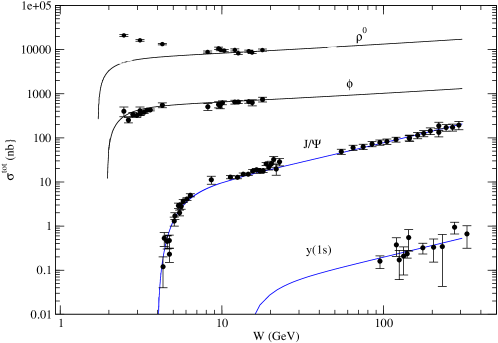
Figure 1: Fits to the data of the total cross sections ($\sigma^{tot}$) of photo-production of $\rho^{0}$, $\phi$, $J/\Psi$ and $y(1s)$ on the proton target. Data are from Refs.jpsi-1 -phi-4 .

In Fig.1, we see that the data for the $\phi$, $J/\Psi$, and $y(1s)$ production can be described very well by the Pomeron-exchange model. On the other hand, the $\rho$ production data at low energies clearly need other mechanisms such as the meson-exchange mechanisms illustrated in Ref.pich .

It appears that the slop parameter $\alpha_{0}$ for the energy-dependence of the diffractive production of heavy quarks ( $c$ and $b$) is rather different from that for light quarks ($u$, $d$, $s$). It will be interesting to understand this observation.

III VMD-LQCD model

We now use the vector meson dominance (VMD) assumption and the $J/\Psi$-N potential $v_{LQCD}$ of Ref.sasaki to construct a model (VMD-LQCD) to predict the $J/\Psi$ photo-production cross sections. It is defined by the following Hamiltonian (from now on, we also use $V$ to denote $J/\Psi$):

$$H=H_{0}+v_{LQCD}(r)+\frac{em^{2}_{V}}{f_{V}}\int dxA_{\mu}(x)\phi_{V}^{\mu}(x)\,\,,$$ (10)

where $H_{0}$ is the free Hamiltonian, $f_{V=J/\Psi}=11.2$ as in the Pomeron-exchange model of section II, $A_{\mu}(x)$ and $\phi_{V}^{\mu}(x)$ are the field operators of the photon and the considered vector meson, respectively. Within the Hamiltonian formulation of hadron reactionsgw ; feshbach ; msl , the amplitude of $\gamma(\vec{q})+N(-\vec{q})\rightarrow J/\Psi(\vec{q})+N(-\vec{k})$ can then be written as

$$<\vec{k}\lambda_{V}m_{s}|T_{VN,\gamma N}(W)|\vec{q}\lambda_{\gamma}m_{s}^{\prime}> = <\vec{k}\lambda_{V}m_{s}|T_{LQCD}(W)|\vec{q}\lambda_{\gamma}m_{s}^{\prime}>$$ (11)

where

$$<\vec{k}\lambda_{V}m_{s}|T_{LQCD}(W)|\vec{q}\lambda_{\gamma}m_{s}^{\prime}> = <\vec{k},\lambda_{V}m_{s}|t_{VN,VN}(W)|\vec{q},\lambda_{\gamma}m^{\prime}_{s}>\frac{1}{W-E_{N}(q)-E_{V}(k)+i\epsilon}$$ (12)

$$\times[\frac{em^{2}_{V}}{f_{V}}\frac{1}{(2\pi)^{3/2}}\frac{1}{\sqrt{2q}}\frac{1}{\sqrt{2E_{V}(q)}}]\,,$$

where the outgoing vector meson momentum $k=|\vec{k}|$ and the incoming photon momentum $q=|\vec{q}|$ are defined by $W=E_{V}(k)+E_{N}(k)=E_{N}(q)+q$.

The $V+N\rightarrow V+N$ scattering amplitude $<\vec{k},m_{v}m_{s}|t_{VN,VN}(E)|\vec{q},\lambda m^{\prime}_{s}>$ in Eq.(11) is calculated from the potential $v_{LQCD}(r)$ by solving the Lippmann-Schwinger equation

$$t_{VN,VN}(E)=v_{LQCD}+v_{LQCD}\frac{1}{W-H_{0}+i\epsilon}t_{VN,VN}(E)\,.$$ (13)

Note that $|\vec{q}|\neq|\vec{k}|$ and hence $<\vec{k},\lambda_{V}m_{s}|t_{VN,VN}(E)|\vec{q},\lambda_{\gamma}m^{\prime}_{s}>$ in Eq.(11) is a half-off-shell t-matrix and can not be directly determined by the elastic scattering, $V(\vec{k})+N(-\vec{k})\rightarrow V(\vec{k}^{\,\,{}^{\prime}})+N(-\vec{k}^{\,\,{}^{\prime}})$, cross sections defined by

$$\frac{d\sigma_{VN,VN}}{d\Omega}(W) = \frac{(2\pi)^{4}}{k^{2}}\rho^{2}_{V,N}(k)\frac{1}{6}\sum_{\lambda_{V},m_{s}}\sum_{\lambda^{\prime}_{V},m^{\prime}_{s}}|<\vec{k},\lambda_{V}m_{s}|t_{VN,VN}(W)|\vec{k}^{\,\,{}^{\prime}}\lambda^{\prime}_{V}m^{\prime}_{s}>|^{2}$$

where $|\vec{k}^{\,\,{}^{\prime}}|=|\vec{k}|=k$.

In this work, we use $v_{LQCD}(r)$ extracted from a LQCD calculation of Ref.sasaki . Their LQCD data can be approximately fittedsasaki-1 by

$$v_{LQCD}(r)=v_{0}\,\frac{e^{-\alpha\,r}}{r}$$ (15)

We consider the ranges of parameters : $v_{0}=(-0.06,-0.11)$ and $\alpha=(0.3,0.5)$ GeV, as estimated in Ref.sasaki-1 . In left side of Fig.2, we see that the LQCD data presented in Ref.sasaki can be fitted very well with $v_{0}=-0.06$ and $\alpha=0.3$ GeV ( pot-1)). However, the short-range part at $r<$ about 0.4 fm is difficultsasaki-1 to quantify in this LQCD calculation with a lattice spacing $\sim 0.1$ fm. Thus the potential (pot-2) with $v_{0}=-0.11$ and $\alpha=0.5$ GeV which fits only the data at $r>$ about 0.4 fm will also be considered in our calculations.

By using Eq.(15) to solve scattering equation Eq.(13), we can get the matrix elements of $t_{VN,VN}(W)$ for evaluating $\gamma+N\rightarrow J/\Psi+N$ amplitude Eq.(11) and the differential cross sections Eq.(1). The predicted $J/\Psi$ photo-production cross sections are compared with the data in the right side of Fig.2. We see that the results from pot-1 are comparable to the JLab data, and are higher than the results from the Pomeron-exchange model (red dotted curve) in the near threshold region. The results (dashed curve) from pot-2 are much larger than the data. This indicates the importance of LQCD data in the $r<$ about 0.4 fm region . We will discuss this in section V.

In Fig.3, we see that the total cross sections calculated from the VMD-LQCD model using $J/\Psi$-N potentials pot-1 and pot-2 are well below the data in the high energy region. Clearly, it is necessary to extend the VMD-LQCD model to include the mechanisms of Pomeron-exchange model.

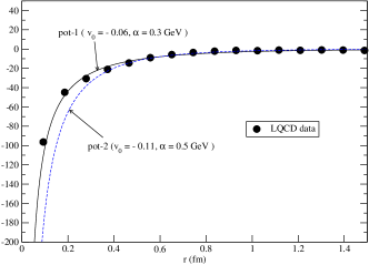
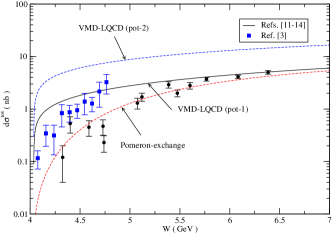
Figure 2: Left: fits to the LQCD data of $J/\Psi$-N potential of Ref.sasaki ; sasaki-1 . $v_{0}$, and $\alpha$ are the parameters of the potential Eq.(15). Right: the total cross sections of $\gamma+p\rightarrow J/\Psi+p$ calculated from VMD-LQCD models with $J/\Psi$-N potentials pot-1 (solid curve) and pot-2 (dashed curve) are compared with the data and the results (dotted curve) from the Pomeron-exchange model presented in section II. The data are from Refs.jpsi-1 -jpsi-4 and jlab .

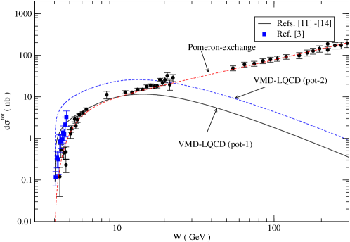
Figure 3: Same as the right-side of Fig.2, except also including the comparisons with the data at high energies.

IV Pomeron-LQCD model

The Pomeron-exchange model developed in Refs.ohlee ; wulee and used here is based on a ”perturbative” analysis of Donnachie and Landshoffdl . Its mechanism is therefore very different from $J/\Psi$-N potential extracted from a LQCD calculation which account for the ”non-perturbative” gluonic interactions between $J/\Psi$ and nucleon. Following the well-established approach in developing models of hadron-hadron scattering, we now extend the Hamiltonian Eq.(10) to develop a model which contain two mechanisms:(1) the ”non-perturbative” $v_{LQCD}$ extracted from LQCD calculation, (2) the ”perturbative” two-gluon-exchange amplitudes of Donnachie and Landshoff which can be generated by a potential $v_{PQCD}$. The $J/\Psi$ photo-production is then defined by the following Hamiltonian:

$$H=H_{0}+[\,v_{LQCD}(r)+v_{PQCD}\,]+\frac{em^{2}_{V}}{f_{V}}\int dxA_{\mu}(x)\phi_{V}^{\mu}(x)$$ (16)

By using the two-potential formula of the well-established reaction theorygw , the amplitude of $J/\Psi$ photo-production derived from Eq.(16) is of the same form of Eq.(11) except that the $V+N\rightarrow V+N$ amplitude is replaced by

$$<\vec{k}|t_{VN,VN}(W)|\vec{q}>\,\,\rightarrow\,\,<\vec{k}|t_{VN,VN}(W)|\vec{q}>+<\vec{k}|t^{PQCD}_{VN,VN}(W)|\vec{q}>\,$$ (17)

where $t_{VN,VN}(W)$ is defined by Eq.(13), and

$$<\vec{k}|t^{PQCD}_{VN,VN}(W)|\vec{q}>=<\phi^{(-)}_{\vec{k},W}|v_{PQCD}|\Psi^{(+)}_{\vec{q},W}>\,,$$ (18)

with

$$<\phi^{(-)}_{\vec{k},W}| = <\vec{k}|[1+v_{LQCD}\frac{1}{W-H_{0}-v_{LQCD}+i\epsilon}]$$ (19)

$$= <\vec{k}|[1+t_{VN,VN}(W)\frac{1}{W-H_{0}+i\epsilon}]$$

and

$$|\Psi^{(+)}_{\vec{q},W}>=[1+\frac{1}{W-H_{0}-v_{LQCD}-v_{PQCD}+i\epsilon}](v_{LQCD}+v_{PQCD})|\vec{k}>\,.$$ (20)

With the replacement Eq.(17), the photo-production amplitude can then be written as

$$<\vec{k}\lambda_{V}m_{s}|T_{VN,\gamma N}(W)|\vec{q}\lambda_{\gamma}m_{s}^{\prime}> = <\vec{k}\lambda_{V}m_{s}|T_{LQCD}(W)|\vec{q}\lambda_{\gamma}m_{s}^{\prime}>$$ (21)

$$+<\vec{k}\lambda_{V}m_{s}|T_{PQCD}(W)|\vec{q}\lambda_{\gamma}m_{s}^{\prime}>$$

where $<\vec{k}\lambda_{V}m_{s}|T_{LQCD}(W)|\vec{q}\lambda_{\gamma}m_{s}^{\prime}>$ is defined by Eq.(12), and

$$<\vec{k}\lambda_{V}m_{s}|T_{PQCD}(W)|\vec{q}\lambda_{\gamma}m_{s}^{\prime}> = <\vec{k},\lambda_{V}m_{s}|t^{PQCD}_{VN,VN}(W)|\vec{q},\lambda_{\gamma}m^{\prime}_{s}>\frac{1}{W-E_{N}(q)-E_{V}(k)+i\epsilon}$$ (22)

$$\times[\frac{em^{2}_{V}}{f_{V}}\frac{1}{(2\pi)^{3/2}}\frac{1}{\sqrt{2q}}\frac{1}{\sqrt{2E_{V}(q)}}]\,,$$

In the absence of a model of $v_{PQCD}$ for solving Eqs.(18)-(20), we assume that the amplitude $<\vec{k}|T_{PQCD}(W)|\vec{q}>$ can be identified with the amplitude of Eq.(LABEL:eq:pomt) of the the Pomeron-exchange model described in section II:

$$<\vec{k}\lambda_{V}m_{s}|T_{PQCD}(W)|\vec{q}\lambda_{\gamma}m_{s}^{\prime}>\,\rightarrow\,<\vec{k}\lambda_{V}m_{s}|T_{P}(W)|\vec{q}\lambda_{\gamma}m_{s}^{\prime}>.$$ (23)

The model defined by Eqs.(16)- Eq.(23) will be refereed to as Pomeron-LQCD model within which the photo-production amplitude is then calculated by using the following form

$$<\vec{k}\lambda_{V}m_{s}|T_{VN,\gamma N}(W)|\vec{q}\lambda_{\gamma}m_{s}^{\prime}> = <\vec{k}\lambda_{V}m_{s}|T_{LQCD}(W)|\vec{q}\lambda_{\gamma}m_{s}^{\prime}>$$ (24)

$$+<\vec{k}\lambda_{V}m_{s}|T_{P}(W)|\vec{q}\lambda_{\gamma}m_{s}^{\prime}>$$

where $<\vec{k}\lambda_{V}m_{s}|T_{LQCD}(W)|\vec{q}\lambda_{\gamma}m_{s}^{\prime}>$ and $<\vec{k}\lambda_{V}m_{s}|T_{P}(W)|\vec{q}\lambda_{\gamma}m_{s}^{\prime}>$ can be calculated by using Eq.(12) and Eq.(LABEL:eq:pomt), respectively.

By using Eq.(24), the $J/\Psi$ photo-production total cross sections are compared with the data in Fig.4. The results from keeping only $T_{LQCD}$ and $T_{P}$ are also shown for comparisons. In the left-side of Fig.4, we see that the contrinution from the amplitude $T_{LQCD}$ dominants the cross sections at low energies. However, it is significantly larger than three JLab data in $W<4.3$ GeV near threshold. At higher energies, it interferes coherently with the Pomeron-exchange contribution (red dashed curve) to give cross sections a little higher than the old data. If pot-2 of $v_{LQCD}$ shown in the left of Fig.2 is used, the calculated total cross sections are a factor of about 5 larger than the JLab data, similar to that (blue dashed curve) shown in the right side of Fig.2.

At high energies, the perturbative amplitude $T_{P}$ dominants and the Pomeron-LQCD model can describe the data as good as the Pomeron-exchange model described in section II. This is shown in the right-side of Fig.4.

We now observe that the best agreements with both the JLab data and earlier data can be obtained by multiplying the VMD constant $1/f_{V}$ in the amplitude Eq.(11) by a factor $F^{off}=0.75$ (0.41) for the calculations using pot-1 (pot-2). These fits are shown in 5. For consistency, the VMD constant in the pomeron-exchange amplitude Eq.(6) should also be multiplied by the same $F^{off}$ factor within Pomeron-LQCD model. This however can be interpreted as just re-defining the Pomeron-quark coupling constant $\beta_{c}\rightarrow\beta_{c}/F^{off}$. We will discuss this $F^{off}$ in the next section.

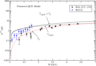
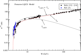
Figure 4: The results (solid curves) from Pomeron-LQCD model are compared with the data. The results from keeping only the amplitude $T_{LQCD}$ (blue dashed curves)and $T_{P}$ (red dashed curves) of Eq.(24) are also shown. Left: from threshold to $W=7$ GeV, Right: from threshold to $W=300$ GeV. The data are from Refs.jpsi-1 -jpsi-4 and jlab .

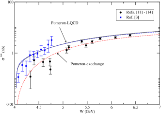
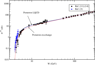
Figure 5: Comparison of the total cross sections calculated from Pomeron-exchange (dotted curves) and Pomeron-LQCD model with $J/\Psi$-N potentials pot-1 (solid curves) and pot-2 (dashed curves). The results from pot-1 (pot-2) are obtained by multiplying $F^{off}=0.75$ (0.41) to VMD coupling constant $1/f_{V}$ to fit the data and are alomst indistinguishable. The data are from Refs.jpsi-1 -jpsi-4 and jlab .

A better way to test the model is to compare the predicted differential cross section $d\sigma/dt$ with the JLab data. In the left side of Fig.6, we see that the results from using $J/\Psi$-N potential pot-1 at three energies in the range of JLab data agree well with the data. In the right side of the same figure, we see that Pomeron-LQCD model can describe the data much better than VMD-LQCD and Pomeron-exchange models.

It will be interesting to test the predictions from Pomeron-LQCD model at energies near threshold. Our predictions at four energies of JLab data are shown in Fig.7. We see that the predictions from Pomeron-exchange model (dashed curves) and Pomeron-LQCD model (solid curves) have rather different $t$-dependence. Hopefully these differences can be tested by the forthcoming data.

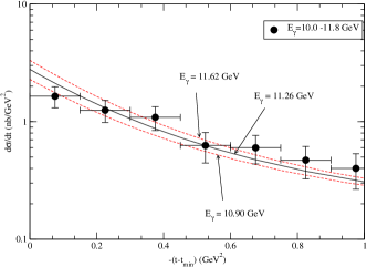
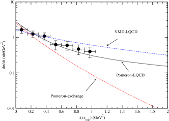
Figure 6: Left: Differential cross sections of $\gamma+p\rightarrow J/\Psi+p$ calculated from the Pomeron-LQCD model are compared with the JLab datajlab . Right:Differential cross sections of $\gamma+p\rightarrow J/\Psi+p$ calculated from the Pomeron-LQCD, VMD-LQCD, and Pomeron-exchange models are compared with the JLab datajlab .

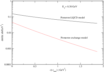
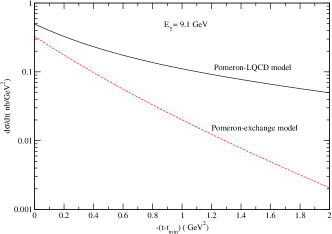
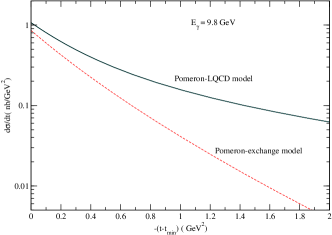
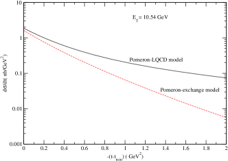
Figure 7: Differential cross sections $\gamma+p\rightarrow J/\Psi+p$ calculated from the Pomeron-LQCD model and Pomeron-exchange model are compared.

V Discussions and necessary improvements

The good agreements with the data shown in Fig.5 are obtained by multiplying the VMD coupling constant $1/f_{V}$ by a factor $F^{off}=075$ and 0.41 for the calculations using $J/\Psi$-N potential pot-1 and pot-2 shown in the left side of Fig.2, respectively. Here we note that the parameter $1/f_{V}$ in Eqs.(6) for Pomeron-exchange model and Eq.(16) for Pomeron-LQCD model is conventionally determined by $V\rightarrow e^{+}e^{-}$ decay width. Thus this coupling is for the photon with $q^{2}=m^{2}_{V}$ which is different from $q^{2}=0$ for the photo-production process considered in this work. It is therefore reasonable to consider that $F^{off}$ is needed phenomenologically to account for this $q^{2}$-dependence of VMD. Since $m^{2}_{J/\Psi}\sim 9$ GeV² is far away from $q^{2}=0$, the factor $F^{off}$ should deviate significantly from 1 and thus the results from pot-2 with a smaller $F^{off}=0.41$ is more reasonable than those from pot-1. If this speculation is correct, a $J/\Psi$-N potential which is more attractive than the data presented in Ref.sasaki is more consistent with Pomeron-LQCD model developed in this work. It will be interesting to have a LQCD calculation which can reduce the uncertainties illustrated in Fig.2.

An another uncertainty of Pomeron-LQCD model is the use of the Yukawa form of Eq.(15) to fit the LQCD data. To see how much our results depend on this choice, we now consider potentials of the following form

$$v(r)=v_{0}(\frac{e^{-\alpha r}}{r}-\frac{e^{\beta r}}{r})$$ (25)

It differs from Eq.(15) in having a finite depth at $r=0$: $v_{0}(0)=v_{0}\times(\beta-\alpha)$. We consider the potentials with $v_{0}=-0.2$ and $\alpha=0.9$ GeV. As shown in the left side of Fig.8, a potential (Fit-1) with $\beta=1.8$ GeV can reproduce the LQCD data as good as pot-1, except that they have very different shapes in the $r<0.2$ fm region. In the right side, we see that the predicted cross sections from these two models are almost indistinguishable. This suggests that in the near threshold region, the predicted cross sections are mainly determined by the potential at $r>$ about 0.2 fm. Thus a LQCD calculation which is accurate for determining the potential down to $r\sim 0.2$ fm will be sufficient for refining the Pomeron-LQCD model.

We next consider two more attractive potentials illustrated in the left side of Fig.9. Their differences with Fit-1 come from using a larger value of $\beta$ in Eq.(25) : $\beta=3.6,6.3$ GeV for Fit-2 and Fit-3, respectively. We see that Fit-2 and Fit-3 only fit the LQCD data at $r>0.3$, and these three potentials have rather different magnitudes at $r=0$. With $F^{off}=1$, the corresponding predictions of $\sigma^{tot}$ are compared in the right side of the same figure. It is clear that the magnitudes of the predicted cross sections increase as the potential becomes more attractive at short distances. Consequently, a smaller $F^{off}$ is needed to fit the data; $F^{off}=0.75,0.4,0.3$ for Fit-1, Fit-2, Fit-3, respectively. This is similar to what we have observed using the potential with Yukawa form Eq.(15) which approaches $\infty$ as $r\rightarrow 0$. Thus the dependence of $F^{off}$ on the attraction of potential is rather independent of the parametrization of the potential in fitting the LQCD data at $r>0.3$ fm.

In summary, we have constructed a Pomeron-LQCD model of $J/\Psi$ photo-production on the nucleon. It is based on the $J/\Psi$ potential extracted from a LQCD calculationsasaki and the amplitudes generated from the Pomeron-exchange model developed in Refs.dl ; ohlee ; wulee . The predicted cross sections are comparable to the recent JLab data at low energies and can also describe the available data up to $W=300$ GeV. However, a off-shell factor $F^{off}$ for accounting for the $q^{2}$-dependence of the VMD constant $1/f_{J/\Psi}$ must be included to explain the JLab data. It is found that this off-shell factor $F^{off}$ sensitively depends on the short-range part of $v_{LQCD}(r)$ at $r<$ about 0.4 fm. To reduce the uncertainties of the Pomeron-LQCD model constructed in this work, we not only need to have information from current LQCD calculations to verify or improve the $v_{LQCD}(r)$ from Ref.sasaki , but also need to find a way to predict $F^{off}$ from a QCD model, such as the $q\bar{q}$-loop model explored in Ref.pich .

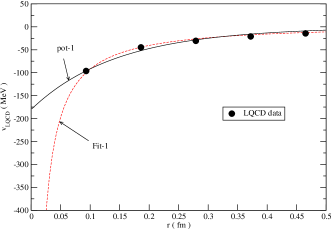
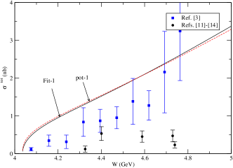
Figure 8: Left: Fits to the LQCD data of $J/\Psi$-N potential of Ref.sasaki ; sasaki-1 . $v_{0}$, $\alpha$, and $\beta$ are the parameters of the potential Eq.(25): $v_{0}=-0.2$, $\alpha=0.9$ GeV, and $\beta=1.8$ GeV for Fit-1. pot-1 is from Fig.2. Right: the predicted total cross sections of $\gamma+p\rightarrow J/\Psi+p$ are compared with the data. $F^{off}$ for the VMD parameter $1/f_{V}$ is set to 1 in these calculations.

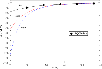
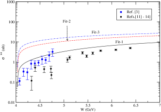
Figure 9: Left: Fits to the LQCD data of $J/\Psi$-N potential of Ref.sasaki . $v_{0}$, $\alpha$, and $\beta$ are the parameters of the potential Eq.(25): $v_{0}=-0.2$, $\alpha=0.9$ GeV and $\beta=1.8,3.6,6.3$ GeV for Fit-1, Fit-2, and Fit-3, respectively. ; Right: the predicted total cross sections of $\gamma+p\rightarrow J/\Psi+p$ are compared with the data. $F^{off}$ for the VMD parameter $1/f_{V}$ is set to 1 in these calculations.