Stochastic processes on surfaces in three-dimensional contact sub-Riemannian manifolds

Davide Barilari, Ugo Boscain, Daniele Cannarsa, Karen Habermann Davide Barilari, Université de Paris, Sorbonne Université, CNRS, Institut de Mathématiques de Jussieu-Paris Rive Gauche, F-75013 Paris, France. davide.barilari@imj-prg.fr Ugo Boscain, CNRS, Laboratoire Jacques-Louis Lions, Sorbonne Université, Université de Paris, Inria, F-75005 Paris, France. ugo.boscain@upmc.fr Daniele Cannarsa, Université de Paris, Sorbonne Université, CNRS, Inria, Institut de Mathématiques de Jussieu-Paris Rive Gauche, F-75013 Paris, France. daniele.cannarsa@imj-prg.fr Karen Habermann, Laboratoire Jacques-Louis Lions, Sorbonne Université, Université de Paris, CNRS, Inria, F-75005 Paris, France. karen.habermann@upmc.fr
Abstract.

We are concerned with stochastic processes on surfaces in three-dimensional contact sub-Riemannian manifolds. Employing the Riemannian approximations to the sub-Riemannian manifold which make use of the Reeb vector field, we obtain a second order partial differential operator on the surface arising as the limit of Laplace–Beltrami operators. The stochastic process associated with the limiting operator moves along the characteristic foliation induced on the surface by the contact distribution. We show that for this stochastic process elliptic characteristic points are inaccessible, while hyperbolic characteristic points are accessible from the separatrices. We illustrate the results with examples and we identify canonical surfaces in the Heisenberg group, and in ${\rm SU}(2)$ and ${\rm SL}(2,\mathbb{R})$ equipped with the standard sub-Riemannian contact structures as model cases for this setting. Our techniques further allow us to derive an expression for an intrinsic Gaussian curvature of a surface in a general three-dimensional contact sub-Riemannian manifold.

1. Introduction

The study of surfaces in three-dimensional contact manifolds has found a lot of interest, amongst others, since the so-called oriented singular foliation on the surface provides an important invariant used to classify contact structures, see Abbas and Hofer [1, Chapter 3], Geiges [17, Chapter 4], and Giroux [18, 19]. In recent years, there has been an increased activity in studying surfaces in three-dimensional contact manifolds whose contact distributions additionally carry a metric. Balogh [4] analyses the Hausdorff dimension of the so-called characteristic set of a hypersurface in the Heisenberg group. Balogh, Tyson and Vecchi [5] define an intrinsic Gaussian curvature for surfaces in the Heisenberg group and an intrinsic signed geodesic curvature for curves on surfaces to obtain a Gauss–Bonnet theorem in the Heisenberg group. Veloso [27] extends the results in [5] to general three-dimensional contact manifolds for non-characteristic surfaces. Danielli, Garofalo and Nhieu [16] discuss the local summability of the sub-Riemannian mean curvature of surfaces in the Heisenberg group. The contribution of this paper is to introduce a canonical stochastic process on a given surface in a three-dimensional contact manifold whose contact distribution is equipped with a metric, to analyse properties of the induced stochastic process and to identify model cases for this setting.

Let $(M,D,g)$ be a three-dimensional contact sub-Riemannian manifold, that is, we consider a three-dimensional manifold $M$ which is equipped with a sub-Riemannian structure $(D,g)$ that is contact. A sub-Riemannian structure on a manifold $M$ consists of a bracket generating distribution $D\subset TM$ and a smooth fibre inner product $g$ defined on $D$. Such a sub-Riemannian structure is said to be contact if the distribution $D$ is a contact structure on $M$. Under the assumption that $D$ is coorientable, the latter means that there exists a global one-form $\omega$ on $M$ satisfying $\omega\wedge{\mathrm{d}}\omega\not=0$ and such that $D=\operatorname{ker}\omega$. The one-form $\omega$ is called a contact form and the pair $(M,D)$ is called a contact manifold. Throughout, we choose the contact form $\omega$ to be normalised such that ${\mathrm{d}}\omega|_{D}=-\operatorname{vol}_{g}$ for $\operatorname{vol}_{g}$ denoting the Euclidean volume form on $D$ induced by the fibre inner product $g$. Associated with the contact form $\omega$, we have the Reeb vector field $X_{0}$ which is the unique vector field on $M$ satisfying ${\mathrm{d}}\omega(X_{0},\cdot)\equiv 0$ and $\omega(X_{0})\equiv 1$.

Let $S$ be an orientable surface embedded in the contact manifold $(M,D)$. We call a point $x\in S$ a characteristic point of $S$ if the contact plane $D_{x}$ coincides with the tangent space $T_{x}S$. Note that characteristic points are also called singular points, cf. [1] and [17]. We denote the set of all characteristic points of $S$ by $\Gamma(S)$. If $x\in S$ is not a characteristic point then $D_{x}$ and $T_{x}S$ intersect in a one-dimensional subspace. These subspaces induce a singular one-dimensional foliation on $S$, that is, an equivalence class of vector fields which differ by a strictly positive or strictly negative function. This foliation is called the characteristic foliation of $S$ induced by the contact structure $D$. We see that the canonical stochastic process we define on the surface $S$ moves along the characteristic foliation. This process does not hit elliptic characteristic points, whereas a hyperbolic characteristic point is hit subject to an appropriate choice of the starting point. In the dynamical systems terminology, an elliptic point corresponds to a node or a focus, and a hyperbolic point is called a saddle, see Robinson [25].

To construct the canonical stochastic process on $S$, we consider the Riemannian approximations to the sub-Riemannian manifold $(M,D,g)$ which make use of the Reeb vector field $X_{0}$. For $\varepsilon>0$, the Riemannian approximation to $(M,D,g)$ defined uniquely by requiring $\sqrt{\varepsilon}X_{0}$ to be unit-length and to be orthogonal to the distribution $D$ everywhere induces a Riemannian metric $g_{\varepsilon}$ on $S$. This gives rise to the two-dimensional Riemannian manifold $(S,g_{\varepsilon})$ and its Laplace–Beltrami operator $\Delta_{\varepsilon}$. We show that the operators $\Delta_{\varepsilon}$ converge uniformly on compacts in $S\setminus\Gamma(S)$ to an operator $\Delta_{0}$ on $S\setminus\Gamma(S)$, and we study the stochastic process on $S\setminus\Gamma(S)$ whose generator is $\frac{1}{2}\Delta_{0}$.

To simplify the presentation of the paper, we shall assume that the distribution $D$ is trivialisable, that is, globally generated by a pair of vector fields, and we choose vector fields $X_{1}$ and $X_{2}$ such that $(X_{1},X_{2})$ is an oriented orthonormal frame for $D$ with respect to the fibre inner product $g$. By the Cartan formula and due to ${\mathrm{d}}\omega|_{D}=-\operatorname{vol}_{g}$, we have

$$\omega([X_{1},X_{2}])=-{\mathrm{d}}\omega(X_{1},X_{2})=1\;.$$

Since $X_{0}$ is the Reeb vector field, we obtain

$$\omega([X_{0},X_{i}])=-{\mathrm{d}}\omega(X_{0},X_{i})=0\quad\mbox{for }i\in\{1,2\}\;.$$

It follows that there exist functions $c_{ij}^{1},c_{ij}^{2}\colon M\to\mathbb{R}$, for $i,j\in\{0,1,2\}$, such that

(1.1) $\displaystyle[X_{1},X_{2}]$ $\displaystyle=c_{12}^{1}X_{1}+c_{12}^{2}X_{2}+X_{0}\;,$
(1.2) $\displaystyle[X_{0},X_{1}]$ $\displaystyle=c_{01}^{1}X_{1}+c_{01}^{2}X_{2}\;,$
(1.3) $\displaystyle[X_{0},X_{2}]$ $\displaystyle=c_{02}^{1}X_{1}+c_{02}^{2}X_{2}\;.$

In particular, the vector fields $X_{1}$, $X_{2}$ and $[X_{1},X_{2}]$ on $M$ are linearly independent everywhere. The Riemannian approximation to $(M,D,g)$ for $\varepsilon>0$ is then obtained by requiring $(X_{1},X_{2},\sqrt{\varepsilon}X_{0})$ to be a global orthonormal frame. We further suppose that the surface $S$ embedded in $M$ is given by

(1.4) $$S=\{x\in M:u(x)=0\}\quad\mbox{for }u\in C^{2}(M)\mbox{ with }{\mathrm{d}}u\not=0\mbox{ on }S\;.$$

While this might define a surface consisting of multiple connected components, we could always restrict our attention to a single connected component. A point $x\in S$ is a characteristic point if and only if $(X_{1}u)(x)=(X_{2}u)(x)=0$, that is,

(1.5) $$x\in\Gamma(S)\quad\mbox{if and only if}\quad\left((X_{1}u)(x)\right)^{2}+\left((X_{2}u)(x)\right)^{2}=0\;.$$

Consequently, the characteristic set $\Gamma(S)$ is a closed subset of $S$. With $\operatorname{Hess}u$ denoting the horizontal Hessian of $u$ defined by

(1.6) $$\operatorname{Hess}u=\begin{pmatrix}X_{1}X_{1}u&X_{1}X_{2}u\\ X_{2}X_{1}u&X_{2}X_{2}u\end{pmatrix}\;,$$

we can classify the characteristic points of $S$ as follows.

Definition.

A characteristic point $x\in\Gamma(S)$ is called non-degenerate if $\det((\operatorname{Hess}u)(x))\not=0$, it is called elliptic if $\det((\operatorname{Hess}u)(x))>0$, and it is called hyperbolic if $\det((\operatorname{Hess}u)(x))<0$.

With the notations introduced above, we can explicitly write down the expression of a unit-length representative of the characteristic foliation of $S$ induced by the contact structure $D$. Let $\widehat{X}_{S}$ be the vector field on $S\setminus\Gamma(S)$ defined by

(1.7) $$\widehat{X}_{S}=\frac{(X_{2}u)X_{1}-(X_{1}u)X_{2}}{\sqrt{(X_{1}u)^{2}+(X_{2}u)^{2}}}\;.$$

Note that while $\widehat{X}_{S}$ is expressed in terms of $X_{1},X_{2}$ and $u$, it only depends on the sub-Riemannian manifold $(M,D,g)$, the embedded surface $S$ and a choice of sign. It is a vector field on $S\setminus\Gamma(S)$ whose vectors have unit length and lie in $D|_{S}\cap TS$ with a continuous choice of sign. In particular, the vector field $\widehat{X}_{S}$ remains unchanged if $u$ is multiplied by a positive function. Let $b\colon S\setminus\Gamma(S)\to\mathbb{R}$ be the function given by

(1.8) $$b=\frac{X_{0}u}{\sqrt{(X_{1}u)^{2}+(X_{2}u)^{2}}}\;.$$

Similarly to the vector field $\widehat{X}_{S}$, the function $b$ can be understood intrinsically. Let $\widehat{X}^{\perp}_{S}$ be such that $(\widehat{X}_{S},\widehat{X}^{\perp}_{S})$ is an oriented orthonormal frame for $D|_{S\setminus\Gamma(S)}$. The function $b$ is then uniquely given by requiring $b\widehat{X}^{\perp}_{S}-X_{0}$ to be a vector field on $S\setminus\Gamma(S)$. Set

(1.9) $$\Delta_{0}=\widehat{X}_{S}^{2}+b\widehat{X}_{S}\;,$$

which is a second order partial differential operator on $S\setminus\Gamma(S)$. The operator $\Delta_{0}$ is invariant under multiplications of $u$ by functions which do not change its zero set. As stated in the theorem below, it arises as the limiting operator of the Laplace–Beltrami operators $\Delta_{\varepsilon}$ in the limit $\varepsilon\to 0$.

Theorem 1.1.

For any twice differentiable function $f\in C_{c}^{2}(S\setminus\Gamma(S))$ compactly supported in $S\setminus\Gamma(S)$, the functions $\Delta_{\varepsilon}f$ converge uniformly on $S\setminus\Gamma(S)$ to $\Delta_{0}f$ as $\varepsilon\to 0$.

Since the theorem above only concerns twice differentiable functions of compact support in $S\setminus\Gamma(S)$, we do not have to put any additional assumptions on the set of characteristic points of $S$.

Following the definition in Balogh, Tyson and Vecchi [5] for surfaces in the Heisenberg group, we introduce an intrinsic Gaussian curvature $K_{0}$ of a surface in a general three-dimensional contact sub-Riemannian manifold as the limit as $\varepsilon\to 0$ of the Gaussian curvatures $K_{\varepsilon}$ of the Riemannian manifolds $(S,g_{\varepsilon})$. To derive the expression given in the following proposition, we employ the same orthogonal frame exhibited to prove Theorem 1.1.

Proposition 1.2.

Uniformly on compact subsets of $S\setminus\Gamma(S)$, we have

$$K_{0}:=\lim_{\varepsilon\to 0}K_{\varepsilon}=-\widehat{X}_{S}(b)-b^{2}\;.$$

We now consider the canonical stochastic process on $S\setminus\Gamma(S)$ whose generator is $\frac{1}{2}\Delta_{0}$. Assuming that it starts at a fixed point then, up to explosion, the process moves along the unique leaf of the characteristic foliation picked out by the starting point. As shown by the next theorem and the following proposition, for this stochastic process, elliptic characteristic points are inaccessible, while hyperbolic characteristic points are accessible from the separatrices. Recall that what we call hyperbolic characteristic points are known as saddles in the dynamical systems literature, whereas what is referred to as hyperbolic points in their language are non-degenerate characteristic points in our terminology.

Theorem 1.3.

The set of elliptic characteristic points in a surface $S$ embedded in $M$ is inaccessible for the stochastic process with generator $\frac{1}{2}\Delta_{0}$ on $S\setminus\Gamma(S)$.

In Section 4.3, we discuss an example of a surface in the Heisenberg group whose induced stochastic process is killed in finite time if started along the separatrices of the characteristic point. Indeed, this phenomena always occurs in the presence of a hyperbolic characteristic point.

Proposition 1.4.

Suppose that the surface $S$ embedded in $M$ has a hyperbolic characteristic point. Then the stochastic process having generator $\frac{1}{2}\Delta_{0}$ and started on the separatrices of the hyperbolic characteristic point reaches that characteristic point with positive probability.

The Sections 4 and 5 are devoted to illustrating the various behaviours the canonical stochastic process induced on the surface $S$ can show. Besides illustrating Proposition 1.4, we show that three classes of familiar stochastic processes arise when considering a natural choice for the surface $S$ in the three classes of model spaces for three-dimensional sub-Riemannian structures, which are the Heisenberg group $\mathbb{H}$, and the special unitary group ${\rm SU}(2)$ and the special linear group ${\rm SL}(2,\mathbb{R})$ equipped with sub-Riemannian contact structures for fibre inner products differing by a constant multiple. In all these cases, the orthonormal frame $(X_{1},X_{2})$ for the distribution $D$ is formed by two left-invariant vector fields which together with the Reeb vector field $X_{0}$ satisfy, for some $\kappa\in\mathbb{R}$, the commutation relations

$$[X_{1},X_{2}]=X_{0}\;,\quad[X_{0},X_{1}]=\kappa X_{2}\;,\quad[X_{0},X_{2}]=-\kappa X_{1}\;,$$

with $\kappa=0$ in the Heisenberg group, $\kappa>0$ in ${\rm SU}(2)$ and $\kappa<0$ in ${\rm SL}(2,\mathbb{R})$. Associated with each of these Lie groups and their Lie algebras, we have the group exponential map $\exp$ for which we identify a left-invariant vector field with its value at the origin.

Theorem 1.5.

Fix $\kappa\in\mathbb{R}$. For $\kappa\not=0$, let $k\in\mathbb{R}$ with $k>0$ be such that $|\kappa|=4k^{2}$. Set $I=(0,\frac{\pi}{k})$ if $\kappa>0$ and $I=(0,\infty)$ otherwise. In the model space for three-dimensional sub-Riemannian structures corresponding to $\kappa$, we consider the embedded surface $S$ parameterised as

$$S=\{\exp(r\cos\theta X_{1}+r\sin\theta X_{2}):r\in I\mbox{ and }\theta\in[0,2\pi)\}\;.$$

Then the limiting operator $\Delta_{0}$ on $S$ is given by

$$\Delta_{0}=\frac{\partial^{2}}{\partial r^{2}}+b\left(r\right)\frac{\partial}{\partial r}\;,$$

where

$$b(r)=\begin{cases}2k\cot(kr)&\mbox{if }\kappa=4k^{2}\\ \frac{2}{r}&\mbox{if }\kappa=0\\ 2k\coth(kr)&\mbox{if }\kappa=-4k^{2}\\ \end{cases}\;.$$

The stochastic process induced by the operator $\frac{1}{2}\Delta_{0}$ moving along the leaves of the characteristic foliation of $S$ is a Bessel process of order $3$ if $\kappa=0$, a Legendre process of order $3$ if $\kappa>0$ and a hyperbolic Bessel process of order $3$ if $\kappa<0$.

Notably, the stochastic processes recovered in the above theorem are all related to one-dimensional Brownian motion by the same type of Girsanov transformation, with only the sign of a parameter distinguishing between them. For the details, see Revuz and Yor [24, p. 357]. A Bessel process of order $3$ arises by conditioning a one-dimensional Brownian motion started on the positive real line to never hit the origin, whereas a Legendre process of order $3$ is obtained by conditioning a Brownian motion started inside an interval to never hit either endpoint of the interval. The examples making up Theorem 1.5 can be considered as model cases for our setting, and all of them illustrate Theorem 1.3.

Notice that the limiting operator we obtain on the leaves is not the Laplacian associated with the metric structure restricted to the leaves as the latter has no drift term. However, the operator $\Delta_{0}$ restricted to a leaf can be considered as a weighted Laplacian. For a smooth measure $\mu=h^{2}\,{\mathrm{d}}x$ on an interval $I$ of the Euclidean line $\mathbb{R}$, the weighted Laplacian applied to a scalar function $f$ yields

$$\operatorname{div}_{\mu}\left(\frac{\partial f}{\partial x}\right)=\frac{\partial^{2}f}{\partial x^{2}}+\frac{2h^{\prime}(x)}{h(x)}\frac{\partial f}{\partial x}\;.$$

In the model cases above, we have

$$h(r)=\begin{cases}\sin\left(kr\right)&\mbox{if }\kappa=4k^{2}\\ r&\mbox{if }\kappa=0\\ \sinh\left(kr\right)&\mbox{if }\kappa=-4k^{2}\\ \end{cases}\;.$$

We prove Theorem 1.1 and Proposition 1.2 in Section 2, where the proof of the theorem relies on the expression of $\Delta_{\varepsilon}|_{S\setminus\Gamma(S)}$ given in Lemma 2.2 in terms of an orthogonal frame for $T(S\setminus\Gamma(S))$. In Section 3, we prove Theorem 1.3 and Proposition 1.4 using Lemma 3.1 and Lemma 3.2, which expand the function $b\colon S\setminus\Gamma(S)\to\mathbb{R}$ from (1.8) in terms of the arc length along the integral curves of $\widehat{X}_{S}$. The results are illustrated in the last two sections. In Section 4, we study quadric surfaces in the Heisenberg group, whereas in Section 5, we consider canonical surfaces in ${\rm SU}(2)$ and ${\rm SL}(2,\mathbb{R})$ equipped with the standard sub-Riemannian contact structures. The examples establishing Theorem 1.5 are discussed in Section 4.1, Section 5.1 and Section 5.2, with a unified viewpoint presented in Section 5.3.

Acknowledgement.

This work was supported by the Grant ANR-15-CE40-0018 “Sub-Riemannian Geometry and Interactions” of the French ANR. The third author is supported by grants from Région Ile-de-France. The fourth author is supported by the Fondation Sciences Mathématiques de Paris. All four authors would like to thank Robert Neel for illuminating discussions.

2. Family of Laplace–Beltrami operators on the embedded surface

We express the Laplace–Beltrami operators $\Delta_{\varepsilon}$ of the Riemannian manifolds $(S,g_{\varepsilon})$ in terms of two vector fields on the surface $S$ which are orthogonal for each of the Riemannian approximations employing the Reeb vector field. Using these expressions of the Laplace–Beltrami operators $\Delta_{\varepsilon}$ where only the coefficients and not the vector fields depend on $\varepsilon>0$, we prove Theorem 1.1. The orthogonal frame exhibited further allows us to establish Proposition 1.2.

For a vector field $X$ on the manifold $M$, the property $Xu|_{S}\equiv 0$ ensures that $X(x)\in T_{x}S$ for all $x\in S$. Therefore, we see that $F_{1}$ and $F_{2}$ given by

(2.1) $\displaystyle F_{1}$ $\displaystyle=\frac{(X_{2}u)X_{1}-(X_{1}u)X_{2}}{\sqrt{(X_{1}u)^{2}+(X_{2}u)^{2}}}\qquad\mbox{and}$
(2.2) $\displaystyle F_{2}$ $\displaystyle=\frac{(X_{0}u)(X_{1}u)X_{1}+(X_{0}u)(X_{2}u)X_{2}}{(X_{1}u)^{2}+(X_{2}u)^{2}}-X_{0}\;,$

are indeed well-defined vector fields on $S\setminus\Gamma(S)$ due to (1.5) and because we have $F_{1}u|_{S\setminus\Gamma(S)}\equiv 0$ as well as $F_{2}u|_{S\setminus\Gamma(S)}\equiv 0$. Here, $S\setminus\Gamma(S)$ is a manifold itself because the characteristic set $\Gamma(S)$ is a closed subset of $S$. We observe that both $F_{1}$ and $F_{2}$ remain unchanged if the function $u$ defining the surface $S$ is multiplied by a positive function, whereas $F_{1}$ changes sign and $F_{2}$ remains unchanged if $u$ is multiplied by a negative function. Since the zero set of the twice differentiable submersion defining $S$ needs to remain unchanged, these are the only two options which can occur. Observe that the vector field $F_{1}$ on $S\setminus\Gamma(S)$ is nothing but the vector field $\widehat{X}_{S}$ defined in (1.7).

Recalling that $g_{\varepsilon}$ is the restriction to the surface $S$ of the Riemannian metric on $M$ obtained by requiring $(X_{1},X_{2},\sqrt{\varepsilon}X_{0})$ to be a global orthonormal frame, we further obtain

$$g_{\varepsilon}(F_{1},F_{2})=0$$

as well as

(2.3) $$g_{\varepsilon}(F_{1},F_{1})=1\quad\mbox{and}\quad g_{\varepsilon}(F_{2},F_{2})=\frac{(X_{0}u)^{2}}{(X_{1}u)^{2}+(X_{2}u)^{2}}+\frac{1}{\varepsilon}\;.$$

Thus, $(F_{1},F_{2})$ is an orthogonal frame for $T(S\setminus\Gamma(S))$ for each Riemannian manifold $(S,g_{\varepsilon})$. While in general, the frame $(F_{1},F_{2})$ is not orthonormal it has the nice property that it does not depend on $\varepsilon>0$, which aids the analysis of the convergence of the operators $\Delta_{\varepsilon}$ in the limit $\varepsilon\to 0$. Since $F_{1}$ and $F_{2}$ are vector fields on $S\setminus\Gamma(S)$, there exist functions $b_{1},b_{2}\colon S\setminus\Gamma(S)\to\mathbb{R}$, not depending on $\varepsilon>0$, such that

(2.4) $$[F_{1},F_{2}]=b_{1}F_{1}+b_{2}F_{2}\;.$$

Whereas determining the functions $b_{1}$ and $b_{2}$ explicitly from (2.1) and (2.2) is a painful task, we can express them nicely in terms of, following the notations in [7], the characteristic deviation $h$ and a tensor $\eta$ related to the torsion. Let $J\colon D\to D$ be the linear transformation induced by the contact form $\omega$ by requiring that, for vector fields $X$ and $Y$ in the distribution $D$,

(2.5) $$g\left(X,J(Y)\right)={\mathrm{d}}\omega(X,Y)\;.$$

Under the assumption of the existence of the global orthonormal frame $(X_{1},X_{2})$ this amounts to saying that

(2.6) $$J(X_{1})=X_{2}\quad\mbox{and}\quad J(X_{2})=-X_{1}\;.$$

For a unit-length vector field $X$ in the distribution $D$, we use $[X,J(X)]|_{D}$ to denote the restriction of the vector field $[X,J(X)]$ on $M$ to the distribution $D$ and we set

$\displaystyle h(X)$ $\displaystyle=-g\left([X,J(X)]|_{D},X\right)\;,$
$\displaystyle\eta(X)$ $\displaystyle=-g\left([X_{0},X],X\right)\;,$

where the expression for $\eta$ is indeed well-defined because according to (1.2) and (1.3), the vector field $[X_{0},X]$ lies in the distribution $D$.

Lemma 2.1.

For $b\colon S\setminus\Gamma(S)\to\mathbb{R}$ defined by (1.8), we have

$$[F_{1},F_{2}]=-\left(bh(F_{1})+\eta(F_{1})\right)F_{1}-bF_{2}\;,$$

that is, $b_{1}=-bh(F_{1})-\eta(F_{1})$ and $b_{2}=-b$.

Proof.

We first observe that due to (2.6), we can write

$$F_{2}=bJ(F_{1})-X_{0}\;.$$

Using (1.2) and (1.3) as well as (2.5), it follows that

$$\omega\left([F_{1},F_{2}]\right)=\omega\left([F_{1},bJ(F_{1})-X_{0}]\right)=-{\mathrm{d}}\omega(F_{1},bJ(F_{1}))=-g(F_{1},bJ^{2}(F_{1}))=b\;.$$

On the other hand, from (2.1), (2.2) and (2.4), we deduce

$$\omega\left([F_{1},F_{2}]\right)=\omega\left(b_{2}F_{2}\right)=-b_{2}\;,$$

which implies that $b_{2}=-b$, as claimed. It remains to determine $b_{1}$. From (2.5), we see that

$$g(F_{1},J(F_{1}))=-\omega([F_{1},F_{1}])=0\;.$$

Together with (2.4) this yields

$$b_{1}=g\left([F_{1},F_{2}],F_{1}\right)=g\left([F_{1},bJ(F_{1})-X_{0}],F_{1}\right)=bg\left([F_{1},J(F_{1})]|_{D},F_{1}\right)+g\left([X_{0},F_{1}],F_{1}\right)\;,$$

and therefore, we have $b_{1}=-bh(F_{1})-\eta(F_{1})$, as required. ∎

To derive an expression for the Laplace–Beltrami operators $\Delta_{\varepsilon}$ of $(S,g_{\varepsilon})$ restricted to $S\setminus\Gamma(S)$ in terms of the vector fields $F_{1}$ and $F_{2}$, it is helpful to consider the normalised frame associated with the orthogonal frame $(F_{1},F_{2})$. For $\varepsilon>0$ fixed, we define $a_{\varepsilon}\colon S\setminus\Gamma(S)\to\mathbb{R}$ by

(2.7) $$a_{\varepsilon}=\left(\frac{(X_{0}u)^{2}}{(X_{1}u)^{2}+(X_{2}u)^{2}}+\frac{1}{\varepsilon}\right)^{-\frac{1}{2}}$$

and we introduce the vector fields $E_{1}$ and $E_{2,\varepsilon}$ on $S\setminus\Gamma(S)$ given by

(2.8) $$E_{1}=F_{1}\quad\mbox{and}\quad E_{2,\varepsilon}=a_{\varepsilon}F_{2}\;.$$

In the Riemannian manifold $(S,g_{\varepsilon})$, this yields the orthonormal frame $(E_{1},E_{2,\varepsilon})$ for $T(S\setminus\Gamma(S))$.

Lemma 2.2.

For $\varepsilon>0$, the operator $\Delta_{\varepsilon}$ restricted to $S\setminus\Gamma(S)$ can be expressed as

$$\Delta_{\varepsilon}|_{S\setminus\Gamma(S)}=F_{1}^{2}+a_{\varepsilon}^{2}F_{2}^{2}+\left(b-\frac{F_{1}(a_{\varepsilon})}{a_{\varepsilon}}\right)F_{1}-a_{\varepsilon}^{2}\left(bh(F_{1})+\eta(F_{1})\right)F_{2}\;.$$
Proof.

Fix $\varepsilon>0$ and let $\operatorname{div}_{\varepsilon}$ denote the divergence operator on the Riemannian manifold $(S,g_{\varepsilon})$ with respect to the corresponding Riemannian volume form. Since $(E_{1},E_{2,\varepsilon})$ is an orthonormal frame for $T(S\setminus\Gamma(S))$, we have

(2.9) $$\Delta_{\varepsilon}|_{S\setminus\Gamma(S)}=E_{1}^{2}+E_{2,\varepsilon}^{2}+\left(\operatorname{div}_{\varepsilon}E_{1}\right)E_{1}+\left(\operatorname{div}_{\varepsilon}E_{2,\varepsilon}\right)E_{2,\varepsilon}\;.$$

Let $(\nu_{1},\nu_{2,\varepsilon})$ denote the dual to the orthonormal frame $(E_{1},E_{2,\varepsilon})$. Proceeding, for instance, in the same way as in [6, Proof of Proposition 11], we show that, for any vector field $X$ on $S\setminus\Gamma(S)$,

$$\operatorname{div}_{\varepsilon}X=\nu_{1}\left([E_{1},X]\right)+\nu_{2,\varepsilon}\left([E_{2,\varepsilon},X]\right)\;.$$

This together with (2.8) and Lemma 2.1 implies that

$$\operatorname{div}_{\varepsilon}E_{1}=\nu_{2,\varepsilon}\left([a_{\varepsilon}F_{2},F_{1}]\right)=-\nu_{2,\varepsilon}\left(a_{\varepsilon}[F_{1},F_{2}]+F_{1}(a_{\varepsilon})F_{2}\right)=b-\frac{F_{1}(a_{\varepsilon})}{a_{\varepsilon}}$$

as well as

$$\operatorname{div}_{\varepsilon}E_{2,\varepsilon}=\nu_{1}\left([F_{1},a_{\varepsilon}F_{2}]\right)=\nu_{1}\left(a_{\varepsilon}[F_{1},F_{2}]+F_{1}(a_{\varepsilon})F_{2}\right)=-a_{\varepsilon}\left(bh(F_{1})+\eta(F_{1})\right)\;.$$

The desired result follows from (2.8) and (2.9). ∎

Note that $\Delta_{\varepsilon}|_{S\setminus\Gamma(S)}$ in Lemma 2.2 can equivalently be written as

$$\Delta_{\varepsilon}|_{S\setminus\Gamma(S)}=F_{1}^{2}+a_{\varepsilon}^{2}F_{2}^{2}+\left(b-\frac{F_{1}\left(a_{\varepsilon}^{2}\right)}{2a_{\varepsilon}^{2}}\right)F_{1}-a_{\varepsilon}^{2}\left(bh(F_{1})+\eta(F_{1})\right)F_{2}\;.$$

Using Lemma 2.2 we can prove Theorem 1.1.

Proof of Theorem 1.1.

From (1.8) and (2.7), we obtain that

(2.10) $$a_{\varepsilon}^{2}=\left(b^{2}+\frac{1}{\varepsilon}\right)^{-1}=\frac{\varepsilon}{\varepsilon b^{2}+1}\;,$$

which we use to compute

$$\frac{F_{1}(a_{\varepsilon})}{a_{\varepsilon}}=\frac{F_{1}(a_{\varepsilon}^{2})}{2a_{\varepsilon}^{2}}=-\frac{\varepsilon bF_{1}(b)}{\varepsilon b^{2}+1}\;.$$

It follows that

(2.11) $$a_{\varepsilon}^{2}\leq\varepsilon\quad\mbox{as well as}\quad\left|\frac{F_{1}(a_{\varepsilon})}{a_{\varepsilon}}\right|\leq\varepsilon\left|bF_{1}(b)\right|\;.$$

Since $u\in C^{2}(M)$ by assumption, both $b\colon S\setminus\Gamma(S)\to\mathbb{R}$ and $F_{1}(b)\colon S\setminus\Gamma(S)\to\mathbb{R}$ are continuous and therefore bounded on compact subsets of $S\setminus\Gamma(S)$. In a similar way, we argue that the function $b_{1}=-bh(F_{1})-\eta(F_{1})$ is bounded on compact subsets of $S\setminus\Gamma(S)$. Due to (2.11), this implies that, uniformly on compact subsets of $S\setminus\Gamma(S)$,

(2.12) $$\lim_{\varepsilon\to 0}a_{\varepsilon}^{2}=0\;,\quad\lim_{\varepsilon\to 0}\frac{F_{1}(a_{\varepsilon})}{a_{\varepsilon}}=0\quad\mbox{and}\quad\lim_{\varepsilon\to 0}a_{\varepsilon}^{2}\left(bh(F_{1})+\eta(F_{1})\right)=0\;.$$

Let $f\in C_{c}^{2}(S\setminus\Gamma(S))$. We then have $F_{1}f,F_{2}f\in C_{c}^{1}(S\setminus\Gamma(S))$ and $F_{1}^{2}f,F_{2}^{2}f\in C_{c}^{0}(S\setminus\Gamma(S))$. Since the expression (1.9) for $\Delta_{0}$ can be rewritten as

$$\Delta_{0}=F_{1}^{2}+bF_{1}$$

and since the convergence in (2.12) is uniformly on compact subsets of $S\setminus\Gamma(S)$, we deduce from Lemma 2.2 that

$$\lim_{\varepsilon\to 0}\left\|\Delta_{\varepsilon}f-\Delta_{0}f\right\|_{\infty,S\setminus\Gamma(S)}=\lim_{\varepsilon\to 0}\left\|a_{\varepsilon}^{2}F_{2}^{2}f-\frac{F_{1}\left(a_{\varepsilon}\right)}{a_{\varepsilon}}F_{1}f-a_{\varepsilon}^{2}\left(bh(F_{1})+\eta(F_{1})\right)F_{2}f\right\|_{\infty,S\setminus\Gamma(S)}=0\;,$$

that is, the functions $\Delta_{\varepsilon}f$ indeed converge uniformly on $S\setminus\Gamma(S)$ to $\Delta_{0}f$. ∎

Using the orthonormal frames $(E_{1},E_{2,\varepsilon})$, we easily derive the expression given in Proposition 1.2 for the intrinsic Gaussian curvature $K_{0}$ of the surface $S$ in terms of the vector field $\widehat{X}_{S}$ and the function $b$. Unlike the reasoning presented in [5], which further exploits intrinsic symmetries of the Heisenberg group $\mathbb{H}$, our derivation does not rely on the cancellation of divergent quantities and holds for surfaces in any three-dimensional contact sub-Riemannian manifold, cf. [5, Remark 5.3].

Proof of Proposition 1.2.

From Lemma 2.1 and due to (2.4) as well as (2.8), we have

$$[E_{1},E_{2,\varepsilon}]=[F_{1},a_{\varepsilon}F_{2}]=a_{\varepsilon}[F_{1},F_{2}]+F_{1}(a_{\varepsilon})F_{2}=a_{\varepsilon}b_{1}E_{1}+\left(-b+\frac{F_{1}(a_{\varepsilon})}{a_{\varepsilon}}\right)E_{2,\varepsilon}\;.$$

According to the classical formula for the Gaussian curvature of a surface in terms of an orthonormal frame, see e.g. [3, Proposition 4.40], the Gaussian curvature $K_{\varepsilon}$ of the Riemannian manifold $(S,g_{\varepsilon})$ is given by

(2.13) $$K_{\varepsilon}=F_{1}\left(-b+\frac{F_{1}(a_{\varepsilon})}{a_{\varepsilon}}\right)-a_{\varepsilon}F_{2}\left(a_{\varepsilon}b_{1}\right)-\left(a_{\varepsilon}b_{1}\right)^{2}-\left(-b+\frac{F_{1}(a_{\varepsilon})}{a_{\varepsilon}}\right)^{2}\;.$$

We deduce from (2.10) that

$$a_{\varepsilon}F_{2}\left(a_{\varepsilon}\right)=\frac{1}{2}F_{2}\left(a_{\varepsilon}^{2}\right)=-\frac{\varepsilon^{2}bF_{2}(b)}{\left(\varepsilon b^{2}+1\right)^{2}}$$

as well as

$$F_{1}\left(\frac{F_{1}(a_{\varepsilon})}{a_{\varepsilon}}\right)=-F_{1}\left(\frac{\varepsilon bF_{1}(b)}{\varepsilon b^{2}+1}\right)=-\frac{\varepsilon F_{1}\left(bF_{1}(b)\right)}{\varepsilon b^{2}+1}+\frac{2\varepsilon^{2}b^{2}\left(F_{1}(b)\right)^{2}}{\left(\varepsilon b^{2}+1\right)^{2}}\;,$$

which, in addition to (2.11), implies

$$\left|a_{\varepsilon}F_{2}\left(a_{\varepsilon}\right)\right|\leq\varepsilon^{2}\left|bF_{2}(b)\right|\quad\mbox{and}\quad\left|F_{1}\left(\frac{F_{1}(a_{\varepsilon})}{a_{\varepsilon}}\right)\right|\leq\varepsilon\left|F_{1}\left(bF_{1}(b)\right)\right|+2\varepsilon^{2}b^{2}\left(F_{1}(b)\right)^{2}\;.$$

By passing to the limit $\varepsilon\to 0$ in (2.13), the desired expression follows. ∎

Notice that, by construction, the function $b$ and the intrinsic Gaussian curvature $K_{0}$ are related by the Riccati-like equation

$$\dot{b}+b^{2}+K_{0}=0\;,$$

with the notation $\dot{b}=\widehat{X}_{S}(b)$.

3. Canonical stochastic process on the embedded surface

We study the stochastic process with generator $\frac{1}{2}\Delta_{0}$ on $S\setminus\Gamma(S)$. After analysing the behaviour of the drift of the process around non-degenerate characteristic points, we prove Theorem 1.3 and Proposition 1.4.

By construction, the process with generator $\frac{1}{2}\Delta_{0}$ moves along the characteristic foliation of $S$, that is, along the integral curves of the vector field $\widehat{X}_{S}$ on $S\setminus\Gamma(S)$ defined in (1.7). Around a fixed non-degenerate characteristic point $x\in\Gamma(S)$, the behaviour of the canonical stochastic process is determined by how $b\colon S\setminus\Gamma(S)\to\mathbb{R}$ given in (1.8) depends on the arc length along integral curves emanating from $x$. Since the vector fields $X_{1},X_{2}$ and the Reeb vector field $X_{0}$ are linearly independent everywhere, the function $X_{0}u\colon S\to\mathbb{R}$ does not vanish near characteristic points. In particular, we may and do choose the function $u\in C^{2}(M)$ defining the surface $S$ such that $X_{0}u\equiv 1$ in a neighbourhood of $x$.

Understanding the expression for the horizontal Hessian $\operatorname{Hess}u$ in (1.6) as a matrix representation in the dual frame of $(X_{1},X_{2})$, and noting that the linear transformation $J\colon D\to D$ defined in (2.5) has the matrix representation

$$J=\begin{pmatrix}0&-1\\ 1&0\end{pmatrix}\;,$$

we see that

$$\left(\operatorname{Hess}u\right)J=\begin{pmatrix}X_{1}X_{2}u&-X_{1}X_{1}u\\ X_{2}X_{2}u&-X_{2}X_{1}u\end{pmatrix}\;.$$

The dynamics around the characteristic point $x\in\Gamma(S)$ is uniquely determined by the eigenvalues $\lambda_{1}$ and $\lambda_{2}$ of $((\operatorname{Hess}u)(x))J$. Since $x\in\Gamma(S)$ is non-degenerate by assumption both eigenvalues are non-zero, and due to $X_{0}u\equiv 1$ in a neighbourhood of $x$, we further have

(3.1) $$\lambda_{1}+\lambda_{2}=\operatorname{Tr}\left(((\operatorname{Hess}u)(x))J\right)=\left(X_{1}X_{2}u\right)(x)-\left(X_{2}X_{1}u\right)(x)=\left(X_{0}u\right)(x)=1\;.$$

Thus, one of the following three cases occurs, where we use the terminology from [25, Section 4.4] to distinguish between them. In the first case, where the eigenvalues $\lambda_{1}$ and $\lambda_{2}$ are complex conjugate, the characteristic point $x$ is of focus type and the integral curves of $\widehat{X}_{S}$ spiral towards the point $x$. In the second case, where both eigenvalues are real and of positive sign, we call $x\in\Gamma(S)$ of node type, and all integral curves of $\widehat{X}_{S}$ approaching $x$ do so tangentially to the eigendirection corresponding to the smaller eigenvalue, with the exception of the separatrices of the larger eigenvalue. In the third case with the characteristic point $x$ being of saddle type, the two eigenvalues are real but of opposite sign, and the only integral curves of $\widehat{X}_{S}$ approaching $x$ are the separatrices.

Note that an elliptic characteristic point is of focus type or of node type, whereas a hyperbolic characteristic point is of saddle type. Depending on which of theses cases arises, we can determine how the function $b$ depends on the arc length along integral curves of $\widehat{X}_{S}$ emanating from $x$. The choice of the function $u\in C^{2}(M)$ such that $X_{0}u\equiv 1$ in a neighbourhood of $x$ fixes the sign of the vector field $\widehat{X}_{S}$. In particular, an integral curve $\gamma$ of $\widehat{X}_{S}$ which extends continuously to $\gamma(0)=x$ might be defined either on the interval $[0,\delta)$ or on $(-\delta,0]$ for some $\delta>0$. As the derivation presented below works irrespective of the sign of the parameter of $\gamma$, we combine the two cases by writing $\gamma\colon I_{\delta}\to S$ for integral curves of $\widehat{X}_{S}$ extended continuously to $\gamma(0)=x$.

The expansion around a characteristic point of focus type is a result of the fact that the real parts of complex conjugate eigenvalues satisfying (3.1) equal $\frac{1}{2}$.

Lemma 3.1.

Let $x\in\Gamma(S)$ be a non-degenerate characteristic point and suppose that $u\in C^{2}(M)$ is chosen such that $X_{0}u\equiv 1$ in a neighbourhood of $x$. For $\delta>0$, let $\gamma\colon I_{\delta}\to S$ be an integral curve of the vector field $\widehat{X}_{S}$ extended continuously to $\gamma(0)=x$. If the eigenvalues of $((\operatorname{Hess}u)(x))J$ are complex conjugate then, as $s\to 0$,

$$b(\gamma(s))=\frac{2}{s}+O(1)\;.$$
Proof.

Since $X_{0}u\equiv 1$ in a neighbourhood of $x$, we may suppose that $\delta>0$ is chosen small enough such that, for $s\in I_{\delta}\setminus\{0\}$,

$$b(\gamma(s))=\frac{1}{\sqrt{\left(\left(X_{1}u\right)\left(\gamma(s)\right)\right)^{2}+\left(\left(X_{2}u\right)\left(\gamma(s)\right)\right)^{2}}}\;.$$

A direct computation shows

$$\frac{\partial}{\partial s}\left(b(\gamma(s))^{-1}\right)=\widehat{X}_{S}\left(b(\gamma(s))^{-1}\right)=\left(\left(\operatorname{Hess}u\right)\left(\gamma(s)\right)\right)\left(J\left(\widehat{X}_{S}\left(\gamma(s)\right)\right),\widehat{X}_{S}\left(\gamma(s)\right)\right)\;.$$

By the Hartman–Grobman theorem, it follows that, for $s\to 0$,

$$\frac{\partial}{\partial s}\left(b(\gamma(s))^{-1}\right)=\left((\operatorname{Hess}u)(x)\right)\left(J\left(\widehat{X}_{S}\left(\gamma(s)\right)\right),\widehat{X}_{S}\left(\gamma(s)\right)\right)+O(s)\;.$$

As complex conjugate eigenvalues of $((\operatorname{Hess}u)(x))J$ have real part equal to $\frac{1}{2}$ and due to $\widehat{X}_{S}$ being a unit-length vector field, the previous expression simplifies to

(3.2) $$\frac{\partial}{\partial s}\left(b(\gamma(s))^{-1}\right)=\frac{1}{2}+O(s)\;.$$

Since $(X_{1}u)(x)=(X_{2}u)(x)=0$ at the characteristic point $x$, we further have

(3.3) $$\lim_{s\to 0}\frac{1}{b(\gamma(s))}=0\;.$$

A Taylor expansion together with (3.2) and (3.3) then implies that, as $s\to 0$,

$$\frac{1}{b(\gamma(s))}=\frac{s}{2}+O\left(s^{2}\right)\;,$$

which yields, for $s\to 0$,

$$b(\gamma(s))=\frac{2}{s}\left(1+O(s)\right)^{-1}=\frac{2}{s}+O(1)\;,$$

as claimed. ∎

The expansion of the function $b$ around characteristic points of node type or of saddle type depends on along which integral curve of $\widehat{X}_{S}$ we are expanding. By the discussions preceding Lemma 3.1, all possible behaviours are covered by the next result.

Lemma 3.2.

Fix a non-degenerate characteristic point $x\in\Gamma(S)$. For $\delta>0$, let $\gamma\colon I_{\delta}\to S$ be an integral curve of the vector field $\widehat{X}_{S}$ which extends continuously to $\gamma(0)=x$. Assume $u\in C^{2}(M)$ is chosen such that $X_{0}u\equiv 1$ in a neighbourhood of $x$ and suppose $((\operatorname{Hess}u)(x))J$ has real eigenvalues. If the curve $\gamma$ approaches $x$ tangentially to the eigendirection corresponding to the eigenvalue $\lambda_{i}$, for $i\in\{1,2\}$, then, as $s\to 0$,

$$b(\gamma(s))=\frac{1}{\lambda_{i}s}+O(1)\;.$$
Proof.

As in the proof of Lemma 3.1, we obtain, for $\delta>0$ small enough and $s\in I_{\delta}\setminus\{0\}$,

$$\widehat{X}_{S}\left(b(\gamma(s))^{-1}\right)=\left(\left(\operatorname{Hess}u\right)\left(\gamma(s)\right)\right)\left(J\left(\widehat{X}_{S}\left(\gamma(s)\right)\right),\widehat{X}_{S}\left(\gamma(s)\right)\right)\;.$$

Since $\gamma$ is an integral curve of the vector field $\widehat{X}_{S}$, we deduce that

$$\frac{\partial}{\partial s}\left(\frac{1}{b(\gamma(s))}\right)=\left(\left(\operatorname{Hess}u\right)\left(\gamma(s)\right)\right)\left(J\left(\gamma^{\prime}(s)\right),\gamma^{\prime}(s)\right)\;.$$

By Taylor expansion, this together with (3.3) yields, for $s\to 0$,

$$\frac{1}{b(\gamma(s))}=\left(\left(\operatorname{Hess}u\right)(x)\right)\left(J\left(\gamma^{\prime}(0)\right),\gamma^{\prime}(0)\right)s+O\left(s^{2}\right)\;.$$

By assumption, the vector $\gamma^{\prime}(0)\in T_{x}S$ is a unit-length eigenvector of $((\operatorname{Hess}u)(x))J$ corresponding to the eigenvalue $\lambda_{i}$, which has to be non-zero because $x$ is a non-degenerate characteristic point. It follows that

$$\left(\left(\operatorname{Hess}u\right)(x)\right)\left(J\left(\gamma^{\prime}(0)\right),\gamma^{\prime}(0)\right)=\lambda_{i}\not=0\;,$$

which implies, for $s\to 0$,

$$b(\gamma(s))=\frac{1}{\lambda_{i}s}\left(1+O(s)\right)^{-1}=\frac{1}{\lambda_{i}s}+O(1)\;,$$

as required. ∎

Remark 3.3.

We stress Lemma 3.2 does not contradict the positivity of the function $b$ near the point $x$ ensured by the choice of $u\in C^{2}(M)$ such that $X_{0}u\equiv 1$ in neighbourhood of $x$. The derived expansion for $b$ simply implies that on the separatrices corresponding to the negative eigenvalue of a hyperbolic characteristic point, the vector field $\widehat{X}_{S}$ points towards the characteristic point for that choice of $u$, that is, we have $s\in(-\delta,0)$. At the same time, we notice that

$$\frac{\partial^{2}}{\partial s^{2}}+b\left(\gamma(s)\right)\frac{\partial}{\partial s}$$

remains invariant under a change from $s$ to $-s$. Therefore, in our analysis of the one-dimensional diffusion processes induced on integral curves of $\widehat{X}_{S}$, we may again assume that the integral curves are parameterised by a positive parameter. $\square$

With the classification of singular points for stochastic differential equations given by Cherny and Engelbert in [15, Section 2.3], the previous two lemmas provide what is needed to prove Theorem 1.3 and Proposition 1.4. One additional crucial observation is that for a characteristic point of node type both eigenvalues of $\left((\operatorname{Hess}u)(x)\right)J$ are positive and less than one, whereas for a characteristic point of saddle type, the positive eigenvalue is greater than one.

Proof of Theorem 1.3.

Fix an elliptic characteristic point $x\in\Gamma(S)$. For $\delta>0$, let $\gamma\colon[0,\delta]\to S$ be an integral curve of the vector field $\widehat{X}_{S}$ extended continuously to $x=\lim_{s\downarrow 0}\gamma(s)$. Following Cherny and Engelbert [15, Section 2.3], since the one-dimensional diffusion process on $\gamma$ induced by $\frac{1}{2}\Delta_{0}$ has unit diffusivity and drift equal to $\frac{1}{2}b$, we set

(3.4) $$\rho(t)=\exp\left(\int_{t}^{\delta}b(\gamma(s))\,{\mathrm{d}}s\right)\quad\mbox{for }t\in(0,\delta]\;.$$

If the characteristic point $x$ is of node type the real positive eigenvalues $\lambda_{1}$ and $\lambda_{2}$ of $((\operatorname{Hess}u)(x))J$ satisfy $0<\lambda_{1},\lambda_{2}<1$ by (3.1). As $x$ is of focus type or of node type by assumption, Lemma 3.1 and Lemma 3.2 establish the existence of some $\lambda\in\mathbb{R}$ with $0<\lambda<1$ such that, as $s\downarrow 0$,

$$b(\gamma(s))=\frac{1}{\lambda s}+O(1)\;.$$

We deduce, for $\delta>0$ sufficiently small,

$$\rho(t)=\exp\left(\int_{t}^{\delta}\left(\frac{1}{\lambda s}+O\left(1\right)\right)\,{\mathrm{d}}s\right)=\exp\left(\frac{1}{\lambda}\ln\left(\frac{\delta}{t}\right)+O(\delta-t)\right)=\left(\frac{\delta}{t}\right)^{\frac{1}{\lambda}}\left(1+O(\delta-t)\right).$$

Due to $\frac{1}{\lambda}>1$, this implies that

$$\int_{0}^{\delta}\rho(t)\,{\mathrm{d}}t=\infty\;.$$

According to [15, Theorem 2.16 and Theorem 2.17], it follows that the elliptic characteristic point $x$ is an inaccessible boundary point for the one-dimensional diffusion processes induced on the integral curves of $\widehat{X}_{S}$ emanating from $x$. Since $x\in\Gamma(S)$ was an arbitrary elliptic characteristic point, the claimed result follows. ∎

Proof of Proposition 1.4.

We consider the stochastic process with generator $\frac{1}{2}\Delta_{0}$ on $S\setminus\Gamma(S)$ near a hyperbolic point $x\in\Gamma(S)$. Let $\gamma$ be one of the four separatrices of $x$ parameterised by arc length $s\geq 0$ and such that $\gamma(0)=x$. Let $\lambda_{1}$ be the positive eigenvalue and $\lambda_{2}$ be the negative eigenvalue of $((\operatorname{Hess}u)(x))J$. From the trace property (3.1), we see that $\lambda_{1}>1$. By Lemma 3.2 and Remark 3.3, we have, for $i\in\{1,2\}$ and as $s\downarrow 0$,

$$b(\gamma(s))=\frac{1}{\lambda_{i}s}+O(1)\;.$$

As in the previous proof, for $\delta>0$ sufficiently small and $\rho\colon(0,\delta]\to\mathbb{R}$ defined by (3.4), we have

$$\rho(t)=\left(\frac{\delta}{t}\right)^{\frac{1}{\lambda_{i}}}\left(1+O(\delta-t)\right)\;.$$

However, this time, due to $\frac{1}{\lambda_{i}}<1$ for $i\in\{1,2\}$, we obtain

$$\int_{0}^{\delta}\rho(t)\,{\mathrm{d}}t<\infty\;.$$

Using $\frac{1}{\lambda_{1}}>0$, we further compute that, on the separatrices corresponding to the positive eigenvalue,

$$\int_{0}^{\delta}\frac{1+\frac{1}{2}|b(\gamma(t))|}{\rho(t)}\,{\mathrm{d}}t=\int_{0}^{\delta}\frac{t^{\frac{1}{\lambda_{1}}-1}}{2\lambda_{1}\delta^{\frac{1}{\lambda_{1}}}}\left(1+O(t)\right)\,{\mathrm{d}}t<\infty$$

and

$$\int_{0}^{\delta}\frac{|b(\gamma(t))|}{2}\,{\mathrm{d}}t=\infty\;.$$

On the separatrices corresponding to the negative eigenvalue, we have, due to $\frac{1}{\lambda_{2}}<0$,

$$\int_{0}^{\delta}\frac{1+\frac{1}{2}|b(\gamma(t))|}{\rho(t)}\,{\mathrm{d}}t=\int_{0}^{\delta}\frac{t^{\frac{1}{\lambda_{2}}-1}}{2\lambda_{2}\delta^{\frac{1}{\lambda_{2}}}}\left(1+O(t)\right)\,{\mathrm{d}}t=\infty$$

as well as

$$s(t)=\int_{0}^{t}\rho(s)\,{\mathrm{d}}s=\frac{\lambda_{2}\delta^{\frac{1}{\lambda_{2}}}}{\lambda_{2}-1}t^{1-\frac{1}{\lambda_{2}}}\left(1+O(t)\right)$$

and

$$\int_{0}^{\delta}\frac{1+\frac{1}{2}|b(\gamma(t))|}{\rho(t)}s(t)\,{\mathrm{d}}t=\int_{0}^{\delta}\frac{1}{2\left(\lambda_{2}-1\right)}\left(1+O(t)\right)\,{\mathrm{d}}t<\infty\;.$$

Hence, as a consequence of the criterions [15, Theorem 2.12 and Theorem 2.13], the hyperbolic characteristic point $x$ is reached with positive probability by the one-dimensional diffusion processes induced on the separatrices. Thus, the canonical stochastic process started on the separatrices is killed in finite time with positive probability. ∎

4. Stochastic processes on quadric surfaces in the Heisenberg group

Let $\mathbb{H}$ be the first Heisenberg group, that is, the Lie group obtained by endowing $\mathbb{R}^{3}$ with the group law, expressed in Cartesian coordinates,

$$(x_{1},y_{1},z_{1})\ast(x_{2},y_{2},z_{2})=\left(x_{1}+x_{2},y_{1}+y_{2},z_{1}+z_{2}+\frac{1}{2}\left(x_{1}y_{2}-x_{2}y_{1}\right)\right)\;.$$

On $\mathbb{H}$, we consider the two left-invariant vector fields

$$X=\frac{\partial}{\partial x}-\frac{y}{2}\frac{\partial}{\partial z}\qquad\mbox{and}\qquad Y=\frac{\partial}{\partial y}+\frac{x}{2}\frac{\partial}{\partial z}\;,$$

and the contact form

$$\omega={\mathrm{d}}z-\frac{1}{2}\left(x\,{\mathrm{d}}y-y\,{\mathrm{d}}x\right)\;.$$

We note that the vector fields $X$ and $Y$ span the contact distribution $D$ corresponding to $\omega$, that they are orthonormal with respect to the smooth fibre inner product $g$ on $D$ given by

$$g_{(x,y,z)}={\mathrm{d}}x\otimes{\mathrm{d}}x+{\mathrm{d}}y\otimes{\mathrm{d}}y\;,$$

and that

$${\mathrm{d}}\omega|_{D}=-{\mathrm{d}}x\wedge{\mathrm{d}}y=-\operatorname{vol}_{g}\;.$$

Therefore, the Heisenberg group $\mathbb{H}$ understood as the three-dimensional contact sub-Riemannian manifold $(\mathbb{R}^{3},D,g)$ falls into our setting, with $X_{1}=X$, $X_{2}=Y$ and the Reeb vector field

$$X_{0}=\frac{\partial}{\partial z}=[X_{1},X_{2}]\;.$$

In Section 4.1 and in Section 4.2, we discuss paraboloids and ellipsoids of revolution admitting one or two characteristic points, respectively, which are elliptic and of focus type. For these examples, the characteristic foliations can be described by logarithmic spirals in $\mathbb{R}^{2}$ lifted to the paraboloids and spirals between the poles on the ellipsoids, which are loxodromes, also called rhumb lines, on spheres. The induced stochastic processes are the Bessel process of order $3$ for the paraboloids and Legendre-like processes for the ellipsoids moving along the leaves of the characteristic foliation. In Section 4.3, we consider hyperbolic paraboloids where, depending on a parameter, the unique characteristic point is either of saddle type or of node type, and we analyse the induced stochastic processes on the separatrices.

4.1. Paraboloid of revolution

For $a\in\mathbb{R}$, let $S$ be the Euclidean paraboloid of revolution given by the equation $z=a(x^{2}+y^{2})$ for Cartesian coordinates $(x,y,z)$ in the Heisenberg group $\mathbb{H}$. This corresponds to the surface given by (1.4) with $u\colon\mathbb{R}^{3}\to\mathbb{R}$ defined as

$$u(x,y,z)=z-a\left(x^{2}+y^{2}\right)\;.$$

We compute

$$X_{0}u\equiv 1\;,\quad\left(X_{1}u\right)(x,y,z)=-2ax-\frac{y}{2}\quad\mbox{and}\quad\left(X_{2}u\right)(x,y,z)=-2ay+\frac{x}{2}\;,$$

which yields

(4.1) $$\left((X_{1}u)(x,y,z)\right)^{2}+\left((X_{2}u)(x,y,z)\right)^{2}=\frac{1}{4}\left(1+16a^{2}\right)\left(x^{2}+y^{2}\right)\;.$$

Thus, the origin of $\mathbb{R}^{3}$ is the only characteristic point on the paraboloid $S$. It is elliptic and of focus type because $X_{0}u\equiv 1$ and

$$\left(\operatorname{Hess}u\right)J\equiv\begin{pmatrix}\frac{1}{2}&2a\\[3.99994pt] -2a&\frac{1}{2}\end{pmatrix}$$

has eigenvalues $\frac{1}{2}\pm 2a\operatorname{i}$. On $S\setminus\Gamma(S)$, the vector field $\widehat{X}_{S}$ defined by (1.7) can be expressed as

(4.2) $$\widehat{X}_{S}=\frac{1}{\sqrt{\left(1+16a^{2}\right)\left(x^{2}+y^{2}\right)}}\left(\left(x-4ay\right)\frac{\partial}{\partial x}+\left(y+4ax\right)\frac{\partial}{\partial y}+2a\left(x^{2}+y^{2}\right)\frac{\partial}{\partial z}\right)\;.$$

Changing to cylindrical coordinates $(r,\theta,z)$ for $\mathbb{R}^{3}\setminus\{0\}$ with $r>0$, $\theta\in[0,2\pi)$, $z\in\mathbb{R}$ and using

$$r\frac{\partial}{\partial r}=x\frac{\partial}{\partial x}+y\frac{\partial}{\partial y}\quad\mbox{as well as}\quad\frac{\partial}{\partial\theta}=-y\frac{\partial}{\partial x}+x\frac{\partial}{\partial y}\;,$$

the expression (4.2) for the vector field $\widehat{X}_{S}$ simplifies to

$$\widehat{X}_{S}=\frac{1}{\sqrt{1+16a^{2}}}\left(\frac{\partial}{\partial r}+\frac{4a}{r}\frac{\partial}{\partial\theta}+2ar\frac{\partial}{\partial z}\right)\;.$$

From (4.1), we further obtain that the function $b\colon S\setminus\Gamma(S)\to\mathbb{R}$ defined by (1.8) can be written as

$$b(r,\theta,z)=\frac{1}{\sqrt{1+16a^{2}}}\frac{2}{r}\;.$$

Characteristic foliation

The characteristic foliation induced on the paraboloid $S$ of revolution by the contact structure $D$ of the Heisenberg group $\mathbb{H}$ is described through the integral curves of the vector field $\widehat{X}_{S}$, cf. Figure 4.1. Its integral curves are spirals emanating from the origin which can be indexed by $\psi\in[0,2\pi)$ and parameterised by $s\in(0,\infty)$ as follows

(4.3) $$s\mapsto\left(\frac{s}{\sqrt{1+16a^{2}}},4a\ln\left(\frac{s}{\sqrt{1+16a^{2}}}\right)+\psi,\frac{as^{2}}{1+16a^{2}}\right)\;.$$

By construction, the vector field $\widehat{X}_{S}$ is a unit vector field with respect to each metric induced on the surface $S$ from Riemannian approximations of the Heisenberg group. In particular, it follows that the parameter $s\in(0,\infty)$ describes the arc length along the spirals (4.3).
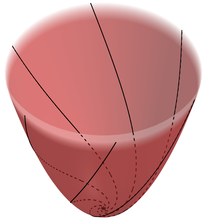
Refer to caption
Figure 4.1. Characteristic foliation described by logarithmic spirals
Remark 4.1.

The spirals on $S$ defined by (4.3) are logarithmic spirals in $\mathbb{R}^{2}$ lifted to the paraboloid of revolution. In polar coordinates $(r,\theta)$ for $\mathbb{R}^{2}$, a logarithmic spiral can be written as

(4.4) $$r=\operatorname{e}^{k\left(\theta+\theta_{0}\right)}\quad\mbox{for }k\in\mathbb{R}\setminus\{0\}\mbox{ and }\theta_{0}\in[0,2\pi)\;.$$

Therefore, the spirals in (4.3) correspond to lifts of logarithmic spirals (4.4) with $k=\frac{1}{4a}$. The arc length $s\in(0,\infty)$ of a logarithmic spiral (4.4) measured from the origin satisfies

$$s=\sqrt{1+\frac{1}{k^{2}}}\,r\;,$$

which for $k=\frac{1}{4a}$ yields $s=\sqrt{1+16a^{2}}\,r.$ Note that this is the same relation between arc length and radial distance as obtained for integral curves (4.3) of the vector field $\widehat{X}_{S}$. For further information on logarithmic spirals, see e.g. Zwikker [29, Chapter 16]. $\square$

Using the spirals (4.3) which describe the characteristic foliation on the paraboloid of revolution, we introduce coordinates $(s,\psi)$ with $s>0$ and $\psi\in[0,2\pi)$ on the surface $S\setminus\Gamma(S)$. The vector field $\widehat{X}_{S}$ on $S\setminus\Gamma(S)$ and the function $b\colon S\setminus\Gamma(S)\to\mathbb{R}$ are then given by

$$\widehat{X}_{S}=\frac{\partial}{\partial s}\quad\mbox{and}\quad b(s,\psi)=\frac{2}{s}\;.$$

Thus, the canonical stochastic process induced on $S\setminus\Gamma(S)$ has generator

$$\frac{1}{2}\Delta_{0}=\frac{1}{2}\left(\widehat{X}_{S}^{2}+b\widehat{X}_{S}\right)=\frac{1}{2}\frac{\partial^{2}}{\partial s^{2}}+\frac{1}{s}\frac{\partial}{\partial s}\;.$$

This gives rise to a Bessel process of order $3$ which out of all the spirals (4.3) describing the characteristic foliation on $S$ stays on the unique spiral passing through the chosen starting point of the induced stochastic process. In agreement with Theorem 1.3, the origin is indeed inaccessible for this stochastic process because a Bessel process of order $3$ with positive starting point remains positive almost surely. It arises as the radial component of a three-dimensional Brownian motion, and it is equal in law to a one-dimensional Brownian motion started on the positive real line and conditioned to never hit the origin. We further observe that the operator $\Delta_{0}$ coincides with the radial part of the Laplace–Beltrami operator for a quadratic cone, cf. [9, 10] for $\alpha=-2$, where the self-adjointness of $\Delta_{0}$ is also studied.

As the limiting operator $\Delta_{0}$ does not depend on the parameter $a\in\mathbb{R}$, the behaviour described above is also what we encounter on the plane $\{z=0\}$ in the Heisenberg group $\mathbb{H}$, where the spirals (4.3) degenerate into rays emanating from the origin. We note that the stochastic process induced by $\frac{1}{2}\Delta_{0}$ on the rays differs from the singular diffusion introduced by Walsh [28] on the same type of structure, but that it falls into the setting of Chen and Fukushima [14].

4.2. Ellipsoid of revolution

For $a,c\in\mathbb{R}$ positive, we study the Euclidean spheroid, also called ellipsoid of revolution, in the Heisenberg group $\mathbb{H}$ given by the equation

$$\frac{x^{2}}{a^{2}}+\frac{y^{2}}{a^{2}}+\frac{z^{2}}{a^{2}c^{2}}=1$$

in Cartesian coordinates $(x,y,z)$. To shorten the subsequent expressions, we choose $u\colon\mathbb{R}^{3}\to\mathbb{R}$ defining the Euclidean spheroid $S$ through (1.4) to be given by

$$u(x,y,z)=x^{2}+y^{2}+\frac{z^{2}}{c^{2}}-a^{2}\;.$$

Proceeding as in the previous example, we first obtain

$$\left(X_{0}u\right)(x,y,z)=\frac{2z}{c^{2}}$$

as well as

$$\left(X_{1}u\right)(x,y,z)=2x-\frac{yz}{c^{2}}\quad\mbox{and}\quad\left(X_{2}u\right)(x,y,z)=2y+\frac{xz}{c^{2}}\;,$$

which yields

(4.5) $$\left((X_{1}u)(x,y,z)\right)^{2}+\left((X_{2}u)(x,y,z)\right)^{2}=\left(x^{2}+y^{2}\right)\left(4+\frac{z^{2}}{c^{4}}\right)\;.$$

This implies the north pole $(0,0,ac)$ and the south pole $(0,0,-ac)$ are the only two characteristic points on the spheroid $S$. We further compute that

(4.6) $$(X_{2}u)X_{1}-(X_{1}u)X_{2}=\left(2y+\frac{xz}{c^{2}}\right)\frac{\partial}{\partial x}-\left(2x-\frac{yz}{c^{2}}\right)\frac{\partial}{\partial y}-\left(x^{2}+y^{2}\right)\frac{\partial}{\partial z}\;.$$

Using adapted spheroidal coordinates $(\theta,\varphi)$ for $S\setminus\Gamma(S)$ with $\theta\in(0,\pi)$ and $\varphi\in[0,2\pi)$, which are related to the coordinates $(x,y,z)$ by

$$x=a\sin(\theta)\cos(\varphi)\;,\quad y=a\sin(\theta)\sin(\varphi)\;,\quad z=ac\cos(\theta)\;,$$

we have

$\displaystyle\frac{a\sin(\theta)}{c}\frac{\partial}{\partial\theta}$ $\displaystyle=\frac{xz}{c^{2}}\frac{\partial}{\partial x}+\frac{yz}{c^{2}}\frac{\partial}{\partial y}-\left(x^{2}+y^{2}\right)\frac{\partial}{\partial z}\quad\mbox{and}$
$\displaystyle\frac{\partial}{\partial\varphi}$ $\displaystyle=-y\frac{\partial}{\partial x}+x\frac{\partial}{\partial y}\;.$

It follows that (4.6) on the surface $S\setminus\Gamma(S)$ simplifies to

$$(X_{2}u)X_{1}-(X_{1}u)X_{2}=\frac{a\sin(\theta)}{c}\frac{\partial}{\partial\theta}-2\frac{\partial}{\partial\varphi}\;,$$

whereas (4.5) on $S\setminus\Gamma(S)$ rewrites as

$$\left((X_{1}u)(\theta,\varphi)\right)^{2}+\left((X_{2}u)(\theta,\varphi)\right)^{2}=a^{2}\left(\sin(\theta)\right)^{2}\left(4+\frac{a^{2}\left(\cos(\theta)\right)^{2}}{c^{2}}\right)\;.$$

This shows that the vector field $\widehat{X}_{S}$ on $S\setminus\Gamma(S)$ defined by (1.7) is given as

(4.7) $$\widehat{X}_{S}=\frac{1}{\sqrt{4c^{2}+a^{2}\left(\cos(\theta)\right)^{2}}}\left(\frac{\partial}{\partial\theta}-\frac{2c}{a\sin(\theta)}\frac{\partial}{\partial\varphi}\right)\;.$$

For the function $b\colon S\setminus\Gamma(S)\to\mathbb{R}$ defined by (1.8), we further obtain that

(4.8) $$b(\theta,\varphi)=\frac{2\cot(\theta)}{\sqrt{4c^{2}+a^{2}\left(\cos(\theta)\right)^{2}}}\;.$$

As in the preceding example, in order to understand the canonical stochastic process induced by the operator $\frac{1}{2}\Delta_{0}$ defined through (1.9), we need to express the vector field $\widehat{X}_{S}$ and the function $b$ in terms of the arc length along the integral curves of $\widehat{X}_{S}$. Since both $\widehat{X}_{S}$ and $b$ are invariant under rotations along the azimuthal angle $\varphi$, this amounts to changing coordinates on the spheroid $S$ from $(\theta,\varphi)$ to $(s,\varphi)$ where $s=s(\theta)$ is uniquely defined by requiring that

$$\frac{\partial}{\partial s}=\frac{1}{\sqrt{4c^{2}+a^{2}\left(\cos(\theta)\right)^{2}}}\left(\frac{\partial}{\partial\theta}-\frac{2c}{a\sin(\theta)}\frac{\partial}{\partial\varphi}\right)\qquad\mbox{and}\qquad s(0)=0\;.$$

This corresponds to

(4.9) $$\frac{{\mathrm{d}}\theta}{{\mathrm{d}}s}=\frac{1}{\sqrt{4c^{2}+a^{2}\left(\cos(\theta)\right)^{2}}}\;,$$

which together with $s(0)=0$ yields

$$s(\theta)=\int_{0}^{\theta}\sqrt{4c^{2}+a^{2}\left(\cos(\tau)\right)^{2}}\,{\mathrm{d}}\tau=\int_{0}^{\theta}\sqrt{\left(4c^{2}+a^{2}\right)-a^{2}\left(\sin(\tau)\right)^{2}}\,{\mathrm{d}}\tau\quad\mbox{for }\theta\in(0,\pi)\;.$$

Hence, the arc length $s$ along the integral curves of $\widehat{X}_{S}$ is given in terms of the polar angle $\theta$ as a multiple of an elliptic integral of the second kind. Consequently, the question if $\theta$ can be expressed explicitly in terms of $s$ is open. However, for our analysis, it is sufficient that the map $\theta\mapsto s(\theta)$ is invertible and that (4.8) as well as (4.9) then imply

$$b(s,\varphi)=2\cot\left(\theta(s)\right)\frac{{\mathrm{d}}\theta}{{\mathrm{d}}s}\;.$$

Therefore, using the coordinates $(s,\varphi)$, the operator $\frac{1}{2}\Delta_{0}$ on $S\setminus\Gamma(S)$ can be expressed as

$$\frac{1}{2}\Delta_{0}=\frac{1}{2}\frac{\partial^{2}}{\partial s^{2}}+\left(\cot\left(\theta(s)\right)\frac{{\mathrm{d}}\theta}{{\mathrm{d}}s}\right)\frac{\partial}{\partial s}\;,$$

which depends on the constants $a,c\in\mathbb{R}$ through (4.9). Without the Jacobian factor $\frac{{\mathrm{d}}\theta}{{\mathrm{d}}s}$ appearing in the drift term, the canonical stochastic process induced by the operator $\frac{1}{2}\Delta_{0}$ and moving along the leaves of the characteristic foliation would be a Legendre process, that is, a Brownian motion started inside an interval and conditioned not to hit either endpoint of the interval. The reason for the appearance of the additional factor $\frac{{\mathrm{d}}\theta}{{\mathrm{d}}s}$ is that the integral curves of $\widehat{X}_{S}$ connecting the two characteristic points are spirals and not just great circles. For some further discussions on the characteristic foliation of the spheroid, see the subsequent Remark 4.3.

The emergence of an operator which is almost the generator of a Legendre process moving along the leaves of the characteristic foliation motivates the search for a surface in a three-dimensional contact sub-Riemannian manifold where we do exhibit a Legendre process moving along the leaves of the characteristic foliation induced by the contact structure. This is achieved in Section 5.1.

Remark 4.2.

The northern hemisphere of the spheroid could equally be defined by the function

$$u(x,y,z)=z-c\sqrt{a^{2}-x^{2}-y^{2}}\;.$$

With this choice we have $X_{0}u\equiv 1$. We further obtain

$$\left(\left(\operatorname{Hess}u\right)(0,0,ac)\right)J=\begin{pmatrix}\frac{1}{2}&-\frac{c}{a}\\[3.99994pt] \frac{c}{a}&\frac{1}{2}\end{pmatrix}\;,$$

whose eigenvalues are 12±caiplus-or-minus12𝑐𝑎i\frac{1}{2}\pm\frac{c}{a}\operatorname{i}. A similar computation on the southern hemisphere implies that both characteristic points are elliptic and of focus type. Thus, by Theorem 1.3, the stochastic process with generator 12Δ012subscriptΔ0\frac{1}{2}\Delta_{0} hits neither the north pole nor the south pole, and it induces a one-dimensional process on the unique leaf of the characteristic foliation picked out by the starting point.
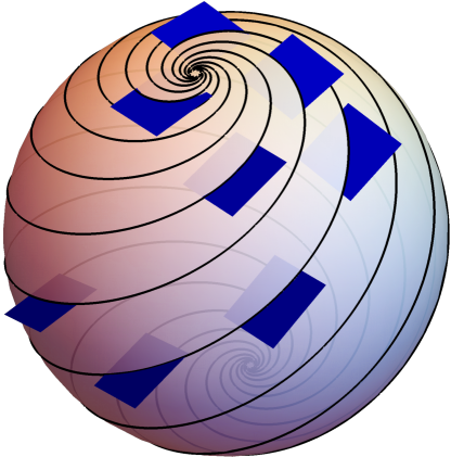
 \square

Remark 4.3.

With respect to the Euclidean metric $\langle\cdot,\cdot\rangle$ on $\mathbb{R}^{3}$, we have for the adapted spheroidal coordinates $(\theta,\varphi)$ of $S\setminus\Gamma(S)$ as above that

$$\left\langle\frac{\partial}{\partial\theta},\frac{\partial}{\partial\theta}\right\rangle=a^{2}\left(\cos(\theta)\right)^{2}+a^{2}c^{2}\left(\sin(\theta)\right)^{2}\quad\mbox{and}\quad\left\langle\frac{\partial}{\partial\varphi},\frac{\partial}{\partial\varphi}\right\rangle=a^{2}\left(\sin(\theta)\right)^{2}\;.$$

It follows that the angle $\alpha$ formed by the vector field $\widehat{X}_{S}$ given in (4.7) and the azimuthal direction satisfies

$$\cos\left(\alpha(\theta,\varphi)\right)=-\frac{2c}{\sqrt{a^{2}\left(\cos(\theta)\right)^{2}+a^{2}c^{2}\left(\sin(\theta)\right)^{2}+4c^{2}}}\;.$$

Notably, on spheres, that is, if $c=1$, the angle $\alpha$ is constant everywhere. Hence, the integral curves of $\widehat{X}_{S}$ considered as Euclidean curves on an Euclidean sphere are loxodromes, cf. Figure 4.2, which are also called rhumb lines. They are related to logarithmic spirals through stereographic projection. Loxodromes arise in navigation by following a path with constant bearing measured with respect to the north pole or the south pole, see Carlton-Wippern [13].

Refer to caption
Figure 4.2. Characteristic foliation on spheres described by loxodromes

\square

4.3. Hyperbolic paraboloid

For $a\in\mathbb{R}$ positive and such that $a\not=\frac{1}{2}$, we consider the Euclidean hyperbolic paraboloid $S$ in the Heisenberg group $\mathbb{H}$ given by (1.4) with $u\colon\mathbb{R}^{3}\to\mathbb{R}$ defined as

$$u(x,y,z)=z-axy\;,$$

for Cartesian coordinates $(x,y,z)$. We compute

(4.10) $$X_{0}u\equiv 1\;,\quad\left(X_{1}u\right)(x,y,z)=-ay-\frac{y}{2}\quad\mbox{as well as}\quad\left(X_{2}u\right)(x,y,z)=-ax+\frac{x}{2}\;,$$

and further that

(4.11) $$\left(\operatorname{Hess}u\right)J\equiv\begin{pmatrix}\frac{1}{2}-a&0\\[3.99994pt] 0&\frac{1}{2}+a\end{pmatrix}\;.$$

Due to

$$\left((X_{1}u)(x,y,z)\right)^{2}+\left((X_{2}u)(x,y,z)\right)^{2}=\left(\frac{1}{2}-a\right)^{2}x^{2}+\left(\frac{1}{2}+a\right)^{2}y^{2}\;,$$

the hyperbolic paraboloid $S$ has the origin of $\mathbb{R}^{3}$ as its unique characteristic point. By (4.11), this characteristic point is elliptic and of node type if $0<a<\frac{1}{2}$, and hyperbolic and therefore of saddle type if $a>\frac{1}{2}$. The reason for having excluded the case $a=\frac{1}{2}$ right from the beginning is that it gives rise to a line of degenerate characteristic points.

We note that the $x$-axis and the $y$-axis lie in the hyperbolic paraboloid $S$. From (4.10), we see that the positive and negative $x$-axis as well as the positive and negative $y$-axis are integral curves of the vector field $\widehat{X}_{S}$ on $S\setminus\Gamma(S)$. In the following, we restrict our attention to studying the behaviour of the canonical stochastic process on these integral curves, which nevertheless nicely illustrates Theorem 1.3 and Proposition 1.4.

We start by analysing the one-dimensional diffusion process induced on the positive $y$-axis $\gamma_{y}^{+}$, which by symmetry is equal in law to the process induced on the negative $y$-axis. For all positive $a\in\mathbb{R}$ with $a\not=\frac{1}{2}$, we have

$$\widehat{X}_{S}|_{\gamma_{y}^{+}}=\frac{\partial}{\partial y}\;,$$

implying that the arc length $s>0$ along $\gamma_{y}^{+}$ is given by $s=y$. This yields, for all $s>0$,

$$b\left(\gamma_{y}^{+}(s)\right)=\frac{1}{\left(\frac{1}{2}+a\right)s}\;.$$

Thus, the one-dimensional diffusion process on $\gamma_{y}^{+}$ induced by $\frac{1}{2}\Delta_{0}$ has generator

$$\frac{1}{2}\frac{\partial^{2}}{\partial s^{2}}+\frac{1}{\left(1+2a\right)s}\frac{\partial}{\partial s}\;,$$

which gives rise to a Bessel process of order $1+\frac{2}{1+2a}$. If started at a point with positive value this diffusion process stays positive for all times almost surely if $1+\frac{2}{1+2a}>2$ whereas it hits the origin with positive probability if $1+\frac{2}{1+2a}<2$. This is consistent with Theorem 1.3 and Proposition 1.4 because for $a>\frac{1}{2}$ the positive $y$-axis is a separatrix for the hyperbolic characteristic point at the origin and

$$2<1+\frac{2}{1+2a}\quad\mbox{if }0<a<\frac{1}{2}\qquad\mbox{as well as}\qquad 2>1+\frac{2}{1+2a}\quad\mbox{if }a>\frac{1}{2}\;.$$

Some more care is needed when studying the diffusion process induced on the positive $x$-axis $\gamma_{x}^{+}$. As before, this process is equal in law to the process induced on the negative $x$-axis. We obtain

$$\widehat{X}_{S}|_{\gamma_{x}^{+}}=\begin{cases}\phantom{-}\frac{\partial}{\partial x}&\mbox{if }0<a<\frac{1}{2}\\[3.99994pt] -\frac{\partial}{\partial x}&\mbox{if }a>\frac{1}{2}\end{cases}$$

as well as, for $x>0$,

$$b(x,0,0)=\begin{cases}\phantom{-}\dfrac{1}{\left(\frac{1}{2}-a\right)x}&\mbox{if }0<a<\frac{1}{2}\\[10.00002pt] -\dfrac{1}{\left(\frac{1}{2}-a\right)x}&\mbox{if }a>\frac{1}{2}\end{cases}\;.$$

It follows that the one-dimensional diffusion process on $\gamma_{x}^{+}$ induced by $\frac{1}{2}\Delta_{0}$ has generator

$$\frac{1}{2}\frac{\partial^{2}}{\partial x^{2}}+\frac{1}{\left(1-2a\right)x}\frac{\partial}{\partial x}\;.$$

This yields a Bessel process of order $1+\frac{2}{1-2a}$. In agreement with Theorem 1.3 and Proposition 1.4, if started at a point with positive value this process never reaches the origin if $0<a<\frac{1}{2}$ which ensures $1+\frac{2}{1-2a}>3$, whereas the process reaches the origin with positive probability if $a>\frac{1}{2}$ as this corresponds to $1+\frac{2}{1-2a}<1$.

5. Stochastic processes on canonical surfaces in ${\rm SU}(2)$ and ${\rm SL}(2,\mathbb{R})$

In Section 4.1, we establish that for a paraboloid of revolution embedded in the Heisenberg group $\mathbb{H}$, the operator $\frac{1}{2}\Delta_{0}$ induces a Bessel process of order $3$ moving along the leaves of the characteristic foliation, which is described by lifts of logarithmic spirals emanating from the origin. As discussed in Revuz and Yor [24, Chapter VIII.3], the Legendre processes and the hyperbolic Bessel processes arise from the same type of Girsanov transformation as the Bessel process, where these three cases only differ by the sign of a parameter. We further recall that in Section 4.2 we encounter a canonical stochastic process which is almost a Legendre process moving along the leaves of the characteristic foliation induced on a spheroid in the Heisenberg group $\mathbb{H}$. This motivates the search for surfaces in three-dimensional contact sub-Riemannian manifolds where the canonical stochastic process is a Legendre process of order $3$ or a hyperbolic Bessel process of order $3$ moving along the leaves of the characteristic foliation.

We consider surfaces in the Lie groups ${\rm SU}(2)$ and ${\rm SL}(2,\mathbb{R})$ endowed with standard sub-Riemannian structures. Together with the Heisenberg group, these sub-Riemannian geometries play the role of model spaces for three-dimensional contact sub-Riemannian manifolds. In the first two subsections, we find, by explicit computations, the canonical stochastic processes induced on certain surfaces in these groups, when expressed in convenient coordinates. The last subsection proposes a unified geometric description, justifying the choice of our surfaces.

5.1. Special unitary group ${\rm SU}(2)$

One obstruction to recovering Legendre processes moving along the characteristic foliation in Section 4.2 is that the characteristic foliation of a spheroid in the Heisenberg group is described by spirals connecting the north pole and the south pole instead of great circles. This is the reason for considering $S^{2}$ as a surface embedded in ${\rm SU}(2)\simeq S^{3}$ understood as a contact sub-Riemannian manifold because this gives rise to a characteristic foliation on $S^{2}$ described by great circles.

The special unitary group ${\rm SU}(2)$ is the Lie group of $2\times 2$ unitary matrices of determinant $1$, that is,

$${\rm SU}(2)=\left\{\begin{pmatrix}\phantom{-}z+w\operatorname{i}&y+x\operatorname{i}\\ -y+x\operatorname{i}&z-w\operatorname{i}\end{pmatrix}\colon x,y,z,w\in\mathbb{R}\mbox{ with }x^{2}+y^{2}+z^{2}+w^{2}=1\right\}\;,$$

with the group operation being given by matrix multiplication. Using the Pauli matrices

$$\sigma_{1}=\begin{pmatrix}0&1\\ 1&0\end{pmatrix}\;,\quad\sigma_{2}=\begin{pmatrix}0&-\operatorname{i}\\ \operatorname{i}&0\end{pmatrix}\quad\mbox{and}\quad\sigma_{3}=\begin{pmatrix}1&0\\ 0&-1\end{pmatrix}\;,$$

we identify ${\rm SU}(2)$ with the unit quaternions, and hence also with $S^{3}$, via the map

$$\begin{pmatrix}\phantom{-}z+w\operatorname{i}&y+x\operatorname{i}\\ -y+x\operatorname{i}&z-w\operatorname{i}\end{pmatrix}\mapsto zI_{2}+x\operatorname{i}\sigma_{1}+y\operatorname{i}\sigma_{2}+w\operatorname{i}\sigma_{3}\;.$$

The Lie algebra $\mathfrak{su}(2)$ of ${\rm SU}(2)$ is the algebra formed by the $2\times 2$ skew-Hermitian matrices with trace zero. A basis for $\mathfrak{su}(2)$ is $\{\frac{\operatorname{i}\sigma_{1}}{2},\frac{\operatorname{i}\sigma_{2}}{2},\frac{\operatorname{i}\sigma_{3}}{2}\}$ and the corresponding left-invariant vector fields on the Lie group ${\rm SU}(2)$ are

$\displaystyle U_{1}$ $\displaystyle=\frac{1}{2}\left(-x\frac{\partial}{\partial z}+z\frac{\partial}{\partial x}-w\frac{\partial}{\partial y}+y\frac{\partial}{\partial w}\right)\;,$
$\displaystyle U_{2}$ $\displaystyle=\frac{1}{2}\left(-y\frac{\partial}{\partial z}+w\frac{\partial}{\partial x}+z\frac{\partial}{\partial y}-x\frac{\partial}{\partial w}\right)\;,$
$\displaystyle U_{3}$ $\displaystyle=\frac{1}{2}\left(-w\frac{\partial}{\partial z}-y\frac{\partial}{\partial x}+x\frac{\partial}{\partial y}+z\frac{\partial}{\partial w}\right)\;,$

which satisfy the commutation relations $[U_{1},U_{2}]=-U_{3}$, $[U_{2},U_{3}]=-U_{1}$ and $[U_{3},U_{1}]=-U_{2}$. Thus, any two of these three left-invariant vector fields give rise to a sub-Riemannian structure on ${\rm SU}(2)$. To streamline the subsequent computations, we choose $k\in\mathbb{R}$ with $k>0$ and equip ${\rm SU}(2)$ with the sub-Riemannian structure obtained by setting $X_{1}=2kU_{1}$, $X_{2}=2kU_{2}$ and by requiring $(X_{1},X_{2})$ to be an orthonormal frame for the distribution $D$ spanned by the vector fields $X_{1}$ and $X_{2}$. The appropriately normalised contact form $\omega$ for the contact distribution $D$ is

$$\omega=\frac{1}{2k^{2}}\left(w\,{\mathrm{d}}z+y\,{\mathrm{d}}x-x\,{\mathrm{d}}y-z\,{\mathrm{d}}w\right)$$

and the associated Reeb vector field $X_{0}$ satisfies

$$X_{0}=[X_{1},X_{2}]=-4k^{2}U_{3}=2k^{2}\left(w\frac{\partial}{\partial z}+y\frac{\partial}{\partial x}-x\frac{\partial}{\partial y}-z\frac{\partial}{\partial w}\right)\;.$$

In ${\rm SU}(2)$, we consider the surface $S$ given by the function $u\colon{\rm SU}(2)\to\mathbb{R}$ defined by

$$u(x,y,z,w)=w\;.$$

The surface $S$ is isomorphic to $S^{2}$ because

$$S=\left\{\begin{pmatrix}z&y+x\operatorname{i}\\ -y+x\operatorname{i}&z\end{pmatrix}\colon x,y,z\in\mathbb{R}\mbox{ with }x^{2}+y^{2}+z^{2}=1\right\}\;.$$

We compute

$$(X_{0}u)(x,y,z,w)=-2k^{2}z\;,\quad(X_{1}u)(x,y,z,w)=ky\quad\mbox{and}\quad(X_{2}u)(x,y,z,w)=-kx\;,$$

which yields

$$\left((X_{1}u)(x,y,z,w)\right)^{2}+\left((X_{2}u)(x,y,z,w)\right)^{2}=k^{2}\left(x^{2}+y^{2}\right)\;.$$

Due to $x^{2}+y^{2}+z^{2}=1$, it follows that a point on $S$ is characteristic if and only if $z=\pm 1$. Thus, the characteristic points on $S$ are the north pole $(0,0,1)$ and the south pole $(0,0,-1)$. The vector field $\widehat{X}_{S}$ on $S\setminus\Gamma(S)$ defined by (1.7) is given as

(5.1) $$\widehat{X}_{S}=\frac{k}{\sqrt{x^{2}+y^{2}}}\left(\left(x^{2}+y^{2}\right)\frac{\partial}{\partial z}-xz\frac{\partial}{\partial x}-yz\frac{\partial}{\partial y}\right)\;,$$

and for the function $b\colon S\setminus\Gamma(S)\to\mathbb{R}$ defined by (1.8), we obtain

(5.2) $$b(x,y,z)=-\frac{2kz}{\sqrt{x^{2}+y^{2}}}\;.$$

We now change coordinates for $S\setminus\Gamma(S)$ from $(x,y,z)$ with $x^{2}+y^{2}+z^{2}=1$ and $z\not=\pm 1$ to $(\theta,\varphi)$ with $\theta\in(0,\frac{\pi}{k})$ and $\varphi\in[0,2\pi)$ by

$$x=\sin(k\theta)\cos(\varphi)\;,\quad y=\sin(k\theta)\sin(\varphi)\quad\mbox{and}\quad z=\cos(k\theta)\;.$$

We note that

$$\frac{\partial}{\partial\theta}=k\cos(k\theta)\cos(\varphi)\frac{\partial}{\partial x}+k\cos(k\theta)\sin(\varphi)\frac{\partial}{\partial y}-k\sin(k\theta)\frac{\partial}{\partial z}$$

as well as

$$xz=\sin(k\theta)\cos(k\theta)\cos(\varphi)\;,\quad yz=\sin(k\theta)\cos(k\theta)\sin(\varphi)\quad\mbox{and}\quad\sqrt{x^{2}+y^{2}}=\sin(k\theta)\;.$$

This together with (5.1) and (5.2) implies that

$$\widehat{X}_{S}=-\frac{\partial}{\partial\theta}\quad\mbox{and}\quad b(\theta,\varphi)=-2k\cot(k\theta)\;.$$

We deduce that the integral curves of $\widehat{X}_{S}$ are great circles on $S$ and that

$$\frac{1}{2}\Delta_{0}=\frac{1}{2}\frac{\partial^{2}}{\partial\theta^{2}}+k\cot(k\theta)\frac{\partial}{\partial\theta}\;,$$

which indeed, on each great circle, induces a Legendre process of order $3$ on the interval $(0,\frac{\pi}{k})$. These processes first appeared in Knight [23] as so-called taboo processes and are obtained by conditioning Brownian motion started inside the interval $(0,\frac{\pi}{k})$ to never hit either of the two boundary points, see Bougerol and Defosseux [12, Section 5.1]. As discussed in Itô and McKean [21, Section 7.15], they also arise as the latitude of a Brownian motion on the three-dimensional sphere of radius $\frac{1}{k}$.

5.2. Special linear group ${\rm SL}(2,\mathbb{R})$

The appearance of the Bessel process on the plane $\{z=0\}$ in the Heisenberg group $\mathbb{H}$ and of the Legendre processes on a compactified plane in ${\rm SU}(2)$ understood as a contact sub-Riemannian manifold suggests that the hyperbolic Bessel processes arise on planes in the special linear group ${\rm SL}(2,\mathbb{R})$ equipped with a sub-Riemannian structure. This is indeed the case if we consider the standard sub-Riemannian structures on ${\rm SL}(2,\mathbb{R})$ where the flow of the Reeb vector field preserves the distribution and the fibre inner product.

The special linear group ${\rm SL}(2,\mathbb{R})$ of degree two over the field $\mathbb{R}$ is the Lie group of $2\times 2$ matrices with determinant $1$, that is,

$${\rm SL}(2,\mathbb{R})=\left\{\begin{pmatrix}x&y\\ z&w\end{pmatrix}\colon x,y,z,w\in\mathbb{R}\mbox{ with }xw-yz=1\right\}\;,$$

where the group operation is taken to be matrix multiplication. The Lie algebra $\mathfrak{sl}(2,\mathbb{R})$ of ${\rm SL}(2,\mathbb{R})$ is the algebra of traceless $2\times 2$ real matrices. A basis of $\mathfrak{sl}(2,\mathbb{R})$ is formed by the three matrices

$$p=\frac{1}{2}\begin{pmatrix}1&0\\ 0&-1\end{pmatrix}\;,\quad q=\frac{1}{2}\begin{pmatrix}0&1\\ 1&0\end{pmatrix}\quad\mbox{and}\quad j=\frac{1}{2}\begin{pmatrix}0&1\\ -1&0\end{pmatrix}\;,$$

whose corresponding left-invariant vector fields on ${\rm SL}(2,\mathbb{R})$ are

$\displaystyle X$ $\displaystyle=\frac{1}{2}\left(x\frac{\partial}{\partial x}-y\frac{\partial}{\partial y}+z\frac{\partial}{\partial z}-w\frac{\partial}{\partial w}\right)\;,$
$\displaystyle Y$ $\displaystyle=\frac{1}{2}\left(y\frac{\partial}{\partial x}+x\frac{\partial}{\partial y}+w\frac{\partial}{\partial z}+z\frac{\partial}{\partial w}\right)\;,$
$\displaystyle K$ $\displaystyle=\frac{1}{2}\left(-y\frac{\partial}{\partial x}+x\frac{\partial}{\partial y}-w\frac{\partial}{\partial z}+z\frac{\partial}{\partial w}\right)\;.$

These vector fields satisfy the commutation relations $[X,Y]=K$, $[X,K]=Y$ and $[Y,K]=-X$. For $k\in\mathbb{R}$ with $k>0$, we equip ${\rm SL}(2,\mathbb{R})$ with the sub-Riemannian structure obtain by considering the distribution $D$ spanned by $X_{1}=2kX$ and $X_{2}=2kY$ as well as the fibre inner product uniquely given by requiring $(X_{1},X_{2})$ to be a global orthonormal frame. The appropriately normalised contact form corresponding to this choice is

$$\omega=\frac{1}{4k^{2}}\left(z\,{\mathrm{d}}x+w\,{\mathrm{d}}y-x\,{\mathrm{d}}z-y\,{\mathrm{d}}w\right)\;,$$

and the Reeb vector field $X_{0}$ associated with the contact form $\omega$ satisfies

$$X_{0}=[X_{1},X_{2}]=4k^{2}K=2k^{2}\left(-y\frac{\partial}{\partial x}+x\frac{\partial}{\partial y}-w\frac{\partial}{\partial z}+z\frac{\partial}{\partial w}\right)\;.$$

The plane in ${\rm SL}(2,\mathbb{R})$ passing tangentially to the contact distribution through the identity element is the surface $S$ given as (1.4) by the function $u\colon{\rm SL}(2,\mathbb{R})\to\mathbb{R}$ defined by

$$u(x,y,z,w)=y-z\;.$$

Observe that, on $S$, we have the relation $xw=1+y^{2}\geq 1$. Therefore, if a point $(x,y,z,w)$ lies on the surface $S$ then so does the point $(-x,y,z,-w)$, and neither $x$ nor $w$ can vanish on $S$. Thus, the function $u\colon{\rm SL}(2,\mathbb{R})\to\mathbb{R}$ induces a surface consisting of two sheets. By symmetry, we restrict our attention to the sheet containing the $2\times 2$ identity matrix, henceforth referred to as the upper sheet. We compute

$$(X_{1}u)(x,y,z,w)=-k\left(y+z\right)\quad\mbox{and}\quad(X_{2}u)(x,y,z,w)=k\left(x-w\right)\;,$$

as well as

$$(X_{0}u)(x,y,z,w)=2k^{2}\left(x+w\right)\;.$$

We note that

$$\left((X_{1}u)(x,y,z,w)\right)^{2}+\left((X_{2}u)(x,y,z,w)\right)^{2}=k^{2}\left(y+z\right)^{2}+k^{2}\left(x-w\right)^{2}$$

vanishes on $S$ if and only if $y=z=0$ and $x=w$. From $xw=1+y^{2}$, it follows that the surface $S$ admits the two characteristic points $(1,0,0,1)$ and $(-1,0,0,-1)$, that is, one unique characteristic point on each sheet. Following Rogers and Williams [26, Section V.36], we choose coordinates $(r,\theta)$ with $r>0$ and $\theta\in[0,2\pi)$ on the upper sheet of $S\setminus\Gamma(S)$ such that

$\displaystyle x$ $\displaystyle=\cosh\left(kr\right)+\sinh\left(kr\right)\cos(\theta)\;,$
$\displaystyle w$ $\displaystyle=\cosh\left(kr\right)-\sinh\left(kr\right)\cos(\theta)\;,\quad\mbox{and}$
$\displaystyle y$ $\displaystyle=\sinh\left(kr\right)\sin(\theta)\;.$

On the upper sheet of $S\setminus\Gamma(S)$, we obtain

$$(X_{1}u)(r,\theta)=-2k\sinh\left(kr\right)\sin(\theta)\quad\mbox{and}\quad(X_{2}u)(r,\theta)=2k\sinh\left(kr\right)\cos(\theta)\;,$$

which yields

$$\sqrt{\left((X_{1}u)(r,\theta)\right)^{2}+\left((X_{2}u)(r,\theta)\right)^{2}}=2k\sinh\left(kr\right)\;,$$

as well as

$$(X_{0}u)(r,\theta)=4k^{2}\cosh\left(kr\right)\;.$$

A direct computation shows that on the upper sheet of $S\setminus\Gamma(S)$, we have

$$\widehat{X}_{S}=\frac{\partial}{\partial r}\quad\mbox{and}\quad b(r,\theta)=2k\coth\left(kr\right)\;,$$

which implies that

$$\frac{1}{2}\Delta_{0}=\frac{1}{2}\frac{\partial^{2}}{\partial r^{2}}+k\coth\left(kr\right)\frac{\partial}{\partial r}\;.$$

Hence, we recover all hyperbolic Bessel processes of order $3$ as the canonical stochastic processes moving along the leaves of the characteristic foliation of the upper sheet of $S\setminus\Gamma(S)$, and similarly on its lower sheet. For further discussions on hyperbolic Bessel processes, see Borodin [8], Gruet [20], Jakubowski and Wiśniewolski [22], and Revuz and Yor [24, Exercise 3.19]. As for the Bessel process of order $3$ and the Legendre processes of order $3$, the hyperbolic Bessel processes of order $3$ can be defined as the radial component of Brownian motion on three-dimensional hyperbolic spaces.

5.3. A unified viewpoint

The surfaces considered in the last two examples together with the plane $\{z=0\}$ in the Heisenberg group are particular cases of the following construction.

Let $G$ be a three-dimensional Lie group endowed with a contact sub-Riemannian structure whose distribution $D$ is spanned by two left-invariant vector fields $X_{1}$ and $X_{2}$ which are orthonormal for the fibre inner product $g$ defined on $D$. Assume that the commutation relations between $X_{1},X_{2}$ and the Reeb vector field $X_{0}$ are given by, for some $\kappa\in\mathbb{R}$,

$$[X_{1},X_{2}]=X_{0}\;,\quad[X_{0},X_{1}]=\kappa X_{2}\;,\quad[X_{0},X_{2}]=-\kappa X_{1}\;.$$

Under these assumptions the flow of the Reeb vector field $X_{0}$ preserves not only the distribution, namely $\operatorname{e}^{tX_{0}}_{*}D=D$, but also the fibre inner product $g$. The examples presented in Section 4.1 and in Sections 5.1 and 5.2 satisfy the above commutation relations with $\kappa=0$ in the Heisenberg group, and for a parameter $k>0$, with $\kappa=4k^{2}$ in ${\rm SU}(2)$ and $\kappa=-4k^{2}$ in ${\rm SL}(2,\mathbb{R})$. These are the three classes of model spaces for three-dimensional sub-Riemannian structures on Lie groups with respect to local sub-Riemannian isometries, see for instance [3, Chapter 17] and [2] for more details.

In each of the examples concerned, the surface $S$ that we consider can be parameterised as

$\displaystyle S$ $\displaystyle=\left\{\exp(x_{1}X_{1}+x_{2}X_{2}):x_{1},x_{2}\in\mathbb{R}\right\}$
$\displaystyle=\left\{\exp(r\cos\theta X_{1}+r\sin\theta X_{2}):r\geq 0,\theta\in[0,2\pi)\right\}\;.$

Observe that $S$ is automatically smooth, connected, and contains the origin of the group. Under these assumptions, the sub-Riemannian structure is of type $\mathbf{d}\oplus\mathbf{s}$ in the sense of [3, Section 7.7.1], and for $\theta$ fixed, the curve $r\mapsto\exp(r\cos\theta X_{1}+r\sin\theta X_{2})$ is a geodesic parameterised by length. Hence, $r\geq 0$ is the arc length parameter along the corresponding trajectory. It follows that the surface $S$ is ruled by geodesics, each of them having vertical component of the initial covector equal to zero. We refer to [3, Chapter 7] for more details on explicit expressions for sub-Riemannian geodesics in these cases, see also [11].

References

  • [1] Casim Abbas and Helmut Hofer. Holomorphic Curves and Global Questions in Contact Geometry. Birkhäuser Advanced Texts: Basler Lehrbücher. Birkhäuser, 2019.
  • [2] Andrei Agrachev and Davide Barilari. Sub-Riemannian structures on 3D Lie groups. Journal of Dynamical and Control Systems, 18(1):21–44, 2012.
  • [3] Andrei Agrachev, Davide Barilari, and Ugo Boscain. A Comprehensive Introduction to Sub-Riemannian Geometry, volume 181 of Cambridge Studies in Advanced Mathematics. Cambridge University Press, 2019.
  • [4] Zoltán M. Balogh. Size of characteristic sets and functions with prescribed gradient. Journal für die Reine und Angewandte Mathematik, 564:63–83, 2003.
  • [5] Zoltán M. Balogh, Jeremy T. Tyson, and Eugenio Vecchi. Intrinsic curvature of curves and surfaces and a Gauss–Bonnet theorem in the Heisenberg group. Mathematische Zeitschrift, 287(1-2):1–38, 2017.
  • [6] Davide Barilari. Trace heat kernel asymptotics in 3D contact sub-Riemannian geometry. Journal of Mathematical Sciences, 195(3):391–411, 2013.
  • [7] Davide Barilari and Mathieu Kohli. On sub-Riemannian geodesic curvature in dimension three.
    arXiv:1910.13132, 29 Oct 2019.
  • [8] Andrei N. Borodin. Hypergeometric diffusion. Journal of Mathematical Sciences, 159(3):295–304, 2009.
  • [9] Ugo Boscain and Robert W. Neel. Extensions of Brownian motion to a family of Grushin-type singularities. Electronic Communications in Probability, 25:12 pp., 2020.
  • [10] Ugo Boscain and Dario Prandi. Self-adjoint extensions and stochastic completeness of the Laplace-Beltrami operator on conic and anticonic surfaces. Journal of Differential Equations, 260(4):3234–3269, 2016.
  • [11] Ugo Boscain and Francesco Rossi. Invariant Carnot-Caratheodory metrics on $S^{3},\ {\rm SO}(3),\ {\rm SL}(2)$, and lens spaces. SIAM Journal on Control and Optimization, 47(4):1851–1878, 2008.
  • [12] Philippe Bougerol and Manon Defosseux. Pitman transforms and Brownian motion in the interval viewed as an affine alcove. arXiv:1808.09182, 12 Sep 2019.
  • [13] Kitt C. Carlton-Wippern. On Loxodromic Navigation. Journal of Navigation, 45(2):292–297, 1992.
  • [14] Zhen-Qing Chen and Masatoshi Fukushima. One-point reflection. Stochastic Processes and their Applications, 125(4):1368–1393, 2015.
  • [15] Alexander S. Cherny and Hans-Jürgen Engelbert. Singular Stochastic Differential Equations, volume 1858 of Lecture Notes in Mathematics. Springer, Berlin, 2005.
  • [16] Donatella Danielli, Nicola Garofalo, and Duy-Minh Nhieu. Integrability of the sub-Riemannian mean curvature of surfaces in the Heisenberg group. Proceedings of the American Mathematical Society, 140(3):811–821, 2012.
  • [17] Hansjörg Geiges. An Introduction to Contact Topology, volume 109 of Cambridge Studies in Advanced Mathematics. Cambridge University Press, 2008.
  • [18] Emmanuel Giroux. Convexité en topologie de contact. Commentarii Mathematici Helvetici, 66(4):637–677, 1991.
  • [19] Emmanuel Giroux. Structures de contact en dimension trois et bifurcations des feuilletages de surfaces. Inventiones Mathematicae, 141(3):615–689, 2000.
  • [20] Jean-Claude Gruet. A note on hyperbolic von Mises distributions. Bernoulli, 6(6):1007–1020, 2000.
  • [21] Kiyosi Itô and Henry P. McKean. Diffusion Processes and their Sample Paths. Springer, Berlin-New York, 1974. Second printing. Die Grundlehren der mathematischen Wissenschaften, Band 125.
  • [22] Jacek Jakubowski and Maciej Wiśniewolski. On hyperbolic Bessel processes and beyond. Bernoulli, 19(5B):2437–2454, 2013.
  • [23] Frank B. Knight. Brownian local times and taboo processes. Transactions of the American Mathematical Society, 143:173–185, 1969.
  • [24] Daniel Revuz and Marc Yor. Continuous Martingales and Brownian Motion, volume 293 of Grundlehren der Mathematischen Wissenschaften. Springer, Berlin, third edition, 1999.
  • [25] Clark Robinson. Dynamical Systems: Stability, Symbolic Dynamics, and Chaos. Studies in Advanced Mathematics. CRC Press, 1995.
  • [26] L. C. G. Rogers and David Williams. Diffusions, Markov Processes, and Martingales. Volume 2: Itô Calculus. Cambridge Mathematical Library. Cambridge University Press, Cambridge, 2000. Reprint of the second edition.
  • [27] José M. M. Veloso. Limit of Gaussian and normal curvatures of surfaces in Riemannian approximation scheme for sub-Riemannian three dimensional manifolds and Gauss–Bonnet theorem. arXiv:2002.07177, 17 Feb 2020.
  • [28] John B. Walsh. A diffusion with a discontinuous local time. In Temps locaux, number 52-53 in Astérisque, pages 37–45. Société mathématique de France, 1978.
  • [29] Cornelis Zwikker. The Advanced Geometry of Plane Curves and Their Applications. (Formerly titled: Advanced Plane Geometry). Dover Publications, 1963.