Carbon ionization at Gbar pressures: an ab initio perspective on astrophysical high-density plasmas

Abstract

A realistic description of partially-ionized matter in extreme thermodynamic states is critical to model the interior and evolution of the multiplicity of high-density astrophysical objects. Current predictions of its essential property, the ionization degree, rely widely on analytical approximations that have been challenged recently by a series of experiments. Here, we propose a novel ab initio approach to calculate the ionization degree directly from the dynamic electrical conductivity using the Thomas-Reiche-Kuhn sum rule. This Density Functional Theory framework captures genuinely the condensed matter nature and quantum effects typical for strongly-correlated plasmas. We demonstrate this new capability for carbon and hydrocarbon, which most notably serve as ablator materials in inertial confinement fusion experiments aiming at recreating stellar conditions. We find a significantly higher carbon ionization degree than predicted by commonly used models, yet validating the qualitative behavior of the average atom model Purgatorio. Additionally, we find the carbon ionization state to remain unchanged in the environment of fully-ionized hydrogen. Our results will not only serve as benchmark for traditional models, but more importantly provide an experimentally accessible quantity in the form of the electrical conductivity.

I Introduction

Modeling the internal structure and thermal evolution of low-mass stars, brown dwarfs, and massive giant planets requires accurate equation of state data and even more importantly reliable transport properties of warm dense matter Chabrier and Baraffe (1997); Becker et al. (2018). For example, the interplay of convective and radiative transport in low-mass stars is reflected by key plasma quantities such as opacity, electrical conductivity, and absorption coefficients. All those properties can be directly linked to the ionization degree, which is defined as the ratio between the number of free electrons and the sum of all electrons.

The ionization degree can be obtained directly from the Saha equations for the limiting case of the low-density plasma in thermodynamic equilibrium. In this framework, the corresponding ionization energies are defined as the difference between the ground state energy and its continuum of free states. Generally, the ionization energies crucially depend on the temperature and density of a plasma. For example, an increase of the density results in a lowering of the ionization energies with respect to their well-known values for isolated atoms due to correlation effects such as screening of the Coulomb interaction, self-energy, strong ion-ion interactions, and Pauli blocking Zimmermann et al. (1978); Kraeft et al. (1986). This effect is known as Ionization Potential Depression (IPD) and inherit to any theory aiming at predicting the ionization degree, which has been subject of many-particle physics for decades Kraeft et al. (1986); Rogers et al. (1996); Murillo and Weisheit (1998); Crowley (2014). For instance, the simple Debye-Hückel theory for static screening has been combined with the ion sphere model by Ecker and Kröll (EK) Ecker and Kröll (1963) and later improved by Stewart and Pyatt (SP) Stewart and Pyatt Jr. (1966). The predictions of both models differ considerably for high-density plasmas as encountered in the deep interior of astrophysical objects, which are characterized by pressures up to the Gbar range and temperatures of several eV to keV.

Matter under such extreme conditions is notoriously challenging to produce and probe. However, great advances in X-ray techniques have been made over the last decade and have been implemented at high-power laser facilities and free electron lasers (FELs), which are now available for the experimental study of high-density plasmas. For instance, the ionization state of isochorically heated solid aluminum was extracted at temperatures in the range of 10-100 eV by measuring the $K$ edge threshold at the Linac Coherent Light Source (LCLS) Vinko et al. (2012); Ciricosta et al. (2012); Cho et al. (2012). Additionally, the ionization of hot dense aluminum plasmas in the range of 1-10 g/cm³ and 500-700 eV was determined using the ORION laser Hoarty et al. (2013). Experiments performed at the Omega laser facility and National Ignition Facility compressed hydrocarbon (CH) up to 100 Mbar, and obtained the ionization state via X-ray Thomson scattering (XRTS) Fletcher et al. (2014); Kraus et al. (2016a). The same technique was applied at the LCLS to measure the IPD in carbon plasma Kraus et al. (2018). Furthermore, the total intensity of plasma emission in Al and Fe driven by narrow-bandwidth X-ray pulses across a range of wavelengths was utilized to determine the IPD Kasim et al. (2018). Generally, the results of those experiments indicate that rather simple models including IPD based on the EK or SP approaches fail to describe the ionization degree correctly Crowley (2014).

Therefore, novel theoretical concepts for the prediction of the ionization degree are imperatively required and first improvements have been made. For example, a two-step Hartree-Fock-Slater (HFS) approach has been proposed recently Son et al. (2014). It is a combined atomic-solid-plasma model that permits ionization potential depression studies also for single and multiple core hole states Rosmej (2018), or the dynamic ion-ion structure factor Lin et al. (2017). The latter approach has been generalized to include Pauli blocking effects which are important at high densities Röpke et al. (2019). Another route is to characterize ionization by applying molecular dynamics simulations for the ions in combination with electronic structure calculations using density functional theory (DFT-MD) Vinko et al. (2014); Hu (2017); Driver et al. (2018), which is especially well-suited for dense plasmas. So far, all DFT-MD works relied widely on the density of states (DOS), which was used to analyze the evolution of the ionization degree with density and temperature Vinko et al. (2014); Hu (2017); Driver et al. (2018). However, none of these works provided a consistent picture of the ionization degree resolving the recent discussion on IPD in high-density plasmas; see Refs. Iglesias (2014); Hu (2017); Röpke et al. (2019), the comment of Iglesias and Sterne Iglesias and Sterne (2018), and the reply by Hu Hu (2018). This debate is fundamentally related to the question of how to define the ionization degree properly for warm dense matter, which is characterized by densities beyond the applicability range of the Saha equations and its underlying chemical picture.

In this work, we meet this challenge by calculating the ionization degree directly from an experimentally accessible quantity: the dynamic electrical conductivity. This DFT-MD method takes into account the electronic and ionic correlations in a self-consistent way and, in particular, reflects essential features of high-density plasmas such as the existence of energy bands instead of sharp atomic levels and their occupation according to Fermi-Dirac statistics. In contrast to a definition relying entirely on the DOS, our novel approach is based on the Thomas-Reiche-Kuhn (TRK) sum rule and the evaluation of electronic transitions originating solely from electrons within the conduction band. This method, which has, to our knowledge, never been used before, is a step toward precisely modeling matter at high energy densities as occurring, e.g., in inertially confined fusion experiments S. H. Glenzer et al. (2012) or in low-mass stars Chabrier and Baraffe (1997), brown dwarfs, and massive giant planets Becker et al. (2018). Carbon and CH are chosen as exemplary materials relevant to the before-mentioned applications.

II Methods

II.1 Deriving ionization from the dynamic conductivity and the sum rule

The dynamic electrical conductivity, also referred to as optical conductivity, is calculated from the Kubo-Greenwood formula,

$$\begin{split}\sigma^{\textrm{tot}}(\omega)\ &=\frac{2\pi e^{2}}{3V\omega}\sum_{\mathbf{k}\nu\mu}\left(f_{\mathbf{k}\nu}-f_{\mathbf{k}\mu}\right)\left|\bra{\mathbf{k}\nu}\hat{\mathbf{v}}\ket{\mathbf{k}\mu}\right|^{2}\cr&\times\delta\left(E_{\mathbf{k}\mu}-E_{\mathbf{k}\nu}-\hbar\omega\right);\end{split}$$ (1)

which can be derived from linear response theory Kubo (1957); Greenwood (1958); Recoules and Crocombette (2005); Holst et al. (2011). In the above equation, the transition matrix elements $\left|\bra{\mathbf{k}\nu}\hat{\mathbf{v}}\ket{\mathbf{k}\mu}\right|^{2}$ with the velocity operator $\hat{\mathbf{v}}$ are the key components. They reflect the transition probability between the initial eigenstate associated with band $\nu$ and the final eigenstate in band $\mu$ at a particular k point in the Brillouin zone of the simulation box of volume $V$. For a given frequency $\omega$, only states with a positive difference between eigenenergies $E_{\mathbf{k}\mu}$ and $E_{\mathbf{k}\nu}$ contribute to the conductivity. The occupation of initial and final states is weighted with the Fermi-Dirac function $f_{\mathbf{k}\nu}=\left[\exp((E_{\mathbf{k}\nu}-\mu_{\textrm{e}})/k_{B}T)+1\right]^{-1}$, whereas $T$ and $\mu_{\textrm{e}}$ denote the temperature and the chemical potential of the electrons, respectively. Additionally, $e$ and $\hbar$ represent the elementary charge and the reduced Planck constant in Eq. (1).

The resulting dynamical electrical conductivity has to fulfill the well-known Thomas-Reiche-Kuhn (TRK) sum rule for dipole transitions Thomas (1925); Reiche and Thomas (1925); Kuhn (1925); Mahan (2000); Desjarlais et al. (2002),

$$Z^{\textrm{tot}}=\frac{N^{\textrm{tot}}_{\textrm{e}}}{N_{\textrm{i}}}=\frac{2m_{e}V}{\pi e^{2}N_{\textrm{i}}}\int_{0}^{\infty}d\omega\;\sigma^{\textrm{tot}}(\omega)\;.$$ (2)

It yields the ratio between the total number of electrons $N^{\textrm{tot}}_{\textrm{e}}$ and the number of ionic centers in the system $N_{\textrm{i}}$ and establishes an important convergence criterion for the numerical computation of the dynamic electrical conductivity. For the examples chosen in this work, we require charge state values of $Z^{\textrm{tot}}=6$ for carbon and $Z^{\textrm{tot}}=7$ for CH in order to fulfill the TRK sum rule exactly. The number of ionic centers is in both cases $N_{\textrm{i}}=N_{\textrm{C}}=N_{\textrm{CH}}=32$.

Our novel approach separates the dynamic electrical conductivity $\sigma^{\textrm{tot}}$ into three individual parts based on the different nature of electronic transitions in the energy spectrum. Hence, the transition matrix elements for a given k point of the sum in Eq. (1) are divided into contributions attributed to intraband transitions in the conduction (c-c) and valence (v-v) band as well as interband transitions between the valence and conduction band (v-c):

$$\sigma^{\textrm{tot}}(\omega)=\sigma^{\textrm{c-c}}(\omega)+\sigma^{\textrm{v-c}}(\omega)+\sigma^{\textrm{v-v}}(\omega)\;,$$ (3)

whereas each contributions $\textrm{x}=\{\textrm{c-c, v-c, v-v}\}$ is required to fulfill the partial TRK sum rule

$$Z^{\textrm{x}}\equiv\frac{2m_{e}V}{\pi e^{2}N_{\textrm{i}}}\int_{0}^{\infty}d\omega\;\sigma^{\textrm{x}}(\omega).$$ (4)

The individual conductivity contributions can be simply identified by choosing an energy within the energy gap between the valence and conduction band, which is chosen naturally as the center of the gap between the states of interest. For our carbon and CH examples, the gap is always chosen between the clearly identifiable 1s valence and the continuum as conduction states, which already comprise the 2s and 2p states at the considered conditions.

The electrons effectively contributing to the conductivity in the conduction band are the free electrons $N_{e}^{\textrm{free}}$, so that we can identify $\sigma^{\textrm{x}}(\omega)=\sigma^{\textrm{c-c}}(\omega)$ in Eq. (4) and define the ionization state as

$$Z^{\textrm{free}}=\frac{N^{\textrm{free}}_{\textrm{e}}}{N_{\textrm{i}}}\equiv Z^{\textrm{c-c}},$$ (5)

which we propose as a new and suitable measure for this quantity in high-density plasmas.

Finally, we calculate the ionization degree,

$$\alpha=\frac{Z^{\textrm{free}}}{Z^{\textrm{tot}}}=\frac{N^{\textrm{free}}_{\textrm{e}}}{N^{\textrm{tot}}_{\textrm{e}}},$$ (6)

which is consequently defined as the ratio between the number of free and total charge carriers per number of ionic centers $N_{\textrm{i}}$.

II.2 Computational details

The DFT-MD simulations for carbon and CH were performed with the Vienna Ab initio Simulation Package (VASP) Kresse and Hafner (1993, 1994); Kresse and Furthmüller (1996). We considered densities between 20-400 g/cm³ at a temperature of 100 eV resulting in a pressure range between 0.8-65 Gbar. These conditions correspond to a maximum compression ratio of more than 100 and thus, it was crucial to treat all electrons explicitly using the Coulomb potential with a cutoff energy of 15 keV. We considered 32 carbon atoms up to 150 g/cm³ and 64 carbon atoms for the three highest densities starting at 200 g/cm³. For the CH calculations, we added 32 and 64 hydrogen atoms to the respective pure carbon simulations. Additionally, a large number of bands, i.e. typically 800 – 5000 bands, was required to describe the adequately at the high temperature considered here. Each DFT-MD simulation was run for at least 20 000 time steps with a step size of 50 as for carbon and 10 as for CH in order to reflect the ion dynamics properly. A Nosé-Hoover thermostat Nosé (1984) was used to control the ion temperature, the Brillouin zone was evaluated at the Baldereschi mean value point Baldereschi (1973), and we employed the exchange-correlation (XC) functional of Perdew, Burke, and Ernzerhof (PBE) Perdew et al. (1996).
The electrical conductivity was determined from an average over 20 snapshots taken from the DFT-MD simulation per condition, and a Monkhorst-Pack 2x2x2 grid was used to evaluate the Kubo-Greenwood formula, Eq. (1). We performed extensive convergence tests of the DFT-MD simulations with respect to the energy cutoff, number of bands, k point sets, and the number of atoms. Furthermore, we tested the influence of the XC functional used in the DFT cycles by carrying out additional calculations with the LDA and SCAN Sun et al. (2015) functionals. All parameters were chosen such that the TRK sum rule is always fulfilled within 2%, which depends most significantly on the number of explicitly considered bands.

III Results

III.1 Dynamic electrical conductivity and sum rule

In the following, we are demonstrating our novel method for an exemplary single snapshot of a carbon plasma at 50 g/cm³ and 100 eV. In Fig. 1, the total dynamic electrical conductivity obtained with the Kubo-Greenwood approach is shown as solid black line. The curve spans three orders of magnitude over the entire considered energy range and exhibits a pronounced local maximum at about 250 eV, which results from the strong v-c conductivity contribution as becomes apparent upon breaking up the total conductivity into its individual contributions associated with c-c, v-c, and v-v transitions according to Eq. (3). While the c-c contribution dominates the total conductivity at energies below 225 eV, the v-c contribution shows a pronounced threshold behaviour at about 175 eV and starts to prevail at energies above 225 eV. At the same time, the v-v transition contribution is almost negligible and can be associated with hopping processes. These can occur as a result of the partial filling of the 1s states at the extreme densities and temperatures investigated here. This behavior is contrary to the known 0 K concept for solids, where the v-v conductivity has to be zero, since the full occupation of the 1s states leads to a vanishing transition probability due to selection rules.

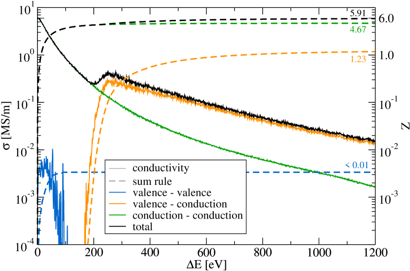
Figure 1: Electrical conductivity (solid lines) and TRK sum rule values (dashed lines) for a carbon simulation snapshot at 50 g/cm³ and $T=100$ eV. The different colors indicate the total value and the individual components of both quantities according to Eq. (3) and Eq. (4). The final TRK sum rule values are given as colored numbers.

Evaluation of the TRK sum rule for the total conductivity according to Eq. (2) yields a value of 5.91, which agrees with the exact sum rule value of 6 within 2 %. The same procedure applied to the v-c contribution results in a value of 1.23, which makes about 21 % to the total sum rule at these conditions. Additionally, the sum rule for the v-v transitions yields a value less than 0.01, which translates to about 0.2 % of the total value, and contributes the most at low energies. Finally,the largest total sum rule contribution of the remaining 79 % is attributed to the sum rule value applied to the c-c conductivity contribution. The resulting c-c value is 4.67 and will be identified as the ionization state later in this work. Note, that all sum rule values given in the following sections are corrected by a factor $Z^{\textrm{exact}}/Z^{\textrm{tot}}$ that accounts for the numerical uncertainty.

III.2 Density of states

In Fig. 2, we show our results for the density of states (DOS) for carbon and CH for all considered densities at 100 eV. Each DOS shows a pronounced valence band corresponding to the 1s states at small energies and the continuum of conduction states at high energies. Note that all energies are plotted with respect to the chemical potential $\mu_{e}$.

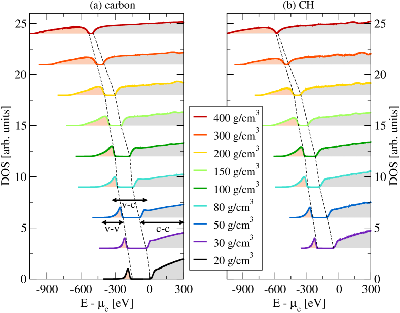
Figure 2: Density of states of carbon (a) and CH (b) for different densities at T = 100 eV. The pink areas indicate states in the 1s valence band, while states in the conduction band are colored in grey. The black arrows show exemplarily at 50 g/cm³ the regions associated with intraband (v-v, c-c) and interband transitions (v-c). The dashed lines serve as guide to the eye for the valence-conduction gap.

For both materials, we observe the valence bands to broaden and shift towards smaller energies with increasing density. At the same time, the edge of the conduction states moves as well towards smaller energies and the gap between valence and conduction bands narrows with rising density. However, the gap never completely vanishes for the considered conditions and can be still clearly identified at the highest considered density of 400 g/cm³.

The center of the gap between valence and conduction bands serves as input for our method to calculate the different conductivity contributions. In principle, any energy in the gap can be used to separate valence from conduction states. In this work, the gap was determined for every snapshot individually via the smallest energy difference between a state in the valence band and one in the conduction state. This approach is formally equivalent to the HOMO-LUMO method, which is applied at T=0 K to obtain the energy difference between highest occupied and lowest unoccupied molecular orbital.

III.3 Conductivity-based Ionization

In Fig. 3 we present our DFT-MD results for the ionization state of dense carbon for a temperature of 100 eV as function of density compared to ionization models that are commonly used for modeling astrophysical or ICF capsule implosions.

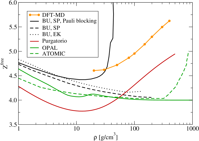
Figure 3: Ionization state of carbon $Z^{\textrm{free}}$ derived from DFT-MD simulations (orange line) according to Eq. (5) compared to predictions of Purgatorio (red line), OPAL (green solid line) Rogers et al. (1996), ATOMIC (green dashed line) Hakel et al. (2006) and Beth-Uhlenbeck (BU) calculations (black lines) Röpke et al. (2019). The BU results incorporate the two different IPD models by Ecker-Kröll (EK) and Stewart-Pyatt (SP), respectively, and the solid line additionally takes into account Pauli blocking effects.

For the lowest densities considered here, the predictions for the carbon ionization state of Purgatorio Sterne et al. (2007), ATOMIC Hakel et al. (2006), OPAL Rogers et al. (1996) and the different Beth-Uhlenbeck (BU) models Röpke et al. (2019) agree qualitatively and predict a decreasing ionization state with increasing density. However, two classes of models can be identified for the high-density regime. On one hand, OPAL and both BU models without Pauli blocking generally continue that trend at densities above 10 g/cm³. Among the three models, OPAL predicts the smallest ionization state and converges towards a constant value of 4. The BU curve including IPD based on the SP model gives slightly higher ionization states, but leads to no essential change in the general behavior compared to the BU approach using the EK description instead. On the other hand, the second class of curves, namely Purgatorio, ATOMIC, the BU model including Pauli blocking as well as our DFT-MD results, is characterized by a steep rise at high densities, which is associated with pressure ionization expected under those conditions Mott (1961). However, the slope and onset of this rise in ionization state vary vastly depending on the approach. The steepest slopes are predicted by ATOMIC and the BU model including Pauli blocking, which in contrast to the other two BU models includes electron degeneracy. While ATOMIC suggests the onset of the increase at about 300 g/cm³, the BU model including Pauli blocking predicts this effect at a density an order of magnitude lower. The DFT-MD results confirm the increase, but the slope of our DFT-MD curve is not as steep. Furthermore, our calculations capture the slope of the average atom model Purgatorio, which evaluates the effective charge at the Wigner Seitz radius Sterne et al. (2007). However, our ab initio calculations yield systematically about 0.5 higher ionization states than Purgatorio indicating that this effective one-particle model is not capturing all important correlation effects treated via our many-body method.

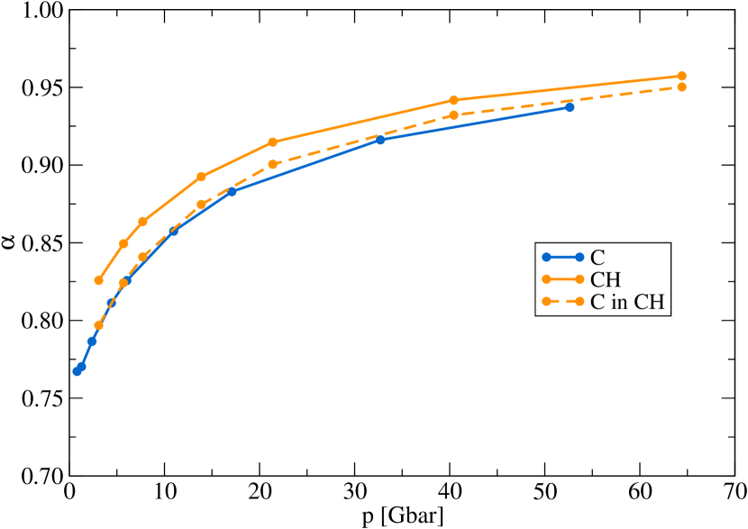
Figure 4: Ionization degree $\alpha$ of pure carbon (blue line), CH (solid orange line), and carbon in CH assuming hydrogen to be fully-ionized (dashed orange line).

The ionization degree derived according to Eq. (6) is shown as a function of pressure for carbon and CH as solid lines in Fig. 4. For both materials, we find a steady increase of the ionization degree in the range of 0.76 to 0.96. Both curves have a very similar slope, while CH yields slightly higher ionization degrees than carbon. Additionally, we plot the ionization degree of the carbon in CH as dashed curve, which agrees remarkably well with the values found for pure carbon indicating that the ionization degree of carbon is not changed by adding hydrogen. Note, that this curve was calculated under the assumption that all hydrogen atoms are fully ionized. This assumption was tested for pure hydrogen at 80 g/cm³, where we find an ionization degree of 1.00 as a result of the conductivity showing only a c-c contribution and of the vanished gap in the DOS.

IV Conclusion

Our presented novel method to derive the ionization state and ionization degree entirely from ab initio simulations by applying the exact TRK sum rule for the dynamic electrical conductivity is entirely self-consistent. This approach naturally takes into account the electronic and ionic correlations, in particular, it reflects essential features of high-density plasmas such as the existence of energy bands instead of sharp atomic levels and their occupation according to Fermi-Dirac statistics. Our DFT-MD results for the carbon ionization state predict a gradually increasing pressure ionization and strongly disagree with commonly used models such as BU Röpke et al. (2019), OPAL Rogers et al. (1996), and ATOMIC Hakel et al. (2006) in high-density plasmas, yet, we confirm the slope of the average atom model Purgatorio Sterne et al. (2007). This indicates that the degeneracy and many-body effects contained in our DFT-MD treatment are crucial to incorporate in any description of the ionization degree and that assumptions based on atomic physics are not valid to treat the ionization balance in high-density plasmas properly. Our conductivity-based method directly exploits knowledge of possible electronic transitions taking into account the nature of the wavefunctions of different states, which cannot be captured by a method that solely relies on the evaluation of the density of states, and additionally provides an experimentally accessible quantity. Hence, the presented data will be useful for analyzing and predicting conditions in inertial confinement fusion experiments using, e.g., the National Ignition Facility. In particular, this data will guide the understanding of XRTS spectra; see Witte et al. (2017); Kraus et al. (2016b).

Finally, the conditions considered in this work, are typically found in high-density astrophysical objects. For instance, densities of 100 g/cm³ and temperatures of 100 eV are expected in the interior of M dwarf stars with a mass of 0.1 M_⊙ (in units of the solar mass). Our results for the ionization degree of carbon and CH can be directly used as input for interior structure models, whose underlying radiation transport models and the nuclear reaction rates crucially rely on ionization models and opacities.

References

- Chabrier and Baraffe (1997) G. Chabrier and I. Baraffe, Astron. Astrophys. 327, 1039 (1997).
- Becker et al. (2018) A. Becker, M. Bethkenhagen, C. Kellermann, J. Wicht, and R. Redmer, Astron. J. 156, 149 (2018).
- Zimmermann et al. (1978) R. Zimmermann, K. Kilimann, W.-D. Kraeft, D. Kremp, and G. Röpke, Phys. Stat. Sol. B 90, 175 (1978).
- Kraeft et al. (1986) W.-D. Kraeft, D. Kremp, W. Ebeling, and G. Röpke, Quantum statistics of charged particle systems (Akademie-Verlag, Berlin, 1986).
- Rogers et al. (1996) F. J. Rogers, F. J. Swenson, and C. A. Iglesias, Astrophys J. 456, 902 (1996).
- Murillo and Weisheit (1998) M. S. Murillo and J. C. Weisheit, Phys. Rep. 302, 1 (1998).
- Crowley (2014) B. J. B. Crowley, High Energy Dens. Phys. 13, 84 (2014).
- Ecker and Kröll (1963) G. Ecker and Kröll, Phys. Fluids 6, 62 (1963).
- Stewart and Pyatt Jr. (1966) J. C. Stewart and K. D. Pyatt Jr., Astrophys. J. 144, 1203 (1966).
- Vinko et al. (2012) S. M. Vinko, O. Ciricosta, B. I. Cho, K. Engelhorn, H.-K. Chung, C. R. D. Brown, T. Burian, J. Chalupsky, R. Falcone, C. Graves, V. Hajkova, A. Higginbotham, L. Juha, J. Krzywinski, H. J. Lee, M. Messerschmidt, C. D. Murphy, Y. Ping, A. Scherz, W. Schlotter, S. Toleikis, J. Turner, L. Vysin, T. Wang, B. Wu, U. Zastrau, D. Zhu, R. W. Lee, P. A. Heimann, B. Nagler, and J. S. Wark, Nature 482, 59 (2012).
- Ciricosta et al. (2012) O. Ciricosta, S. M. Vinko, H.-K. Chung, B.-I. Cho, C. R. D. Brown, T. Burian, J. Chalupsky, K. Engelhorn, R. W. Falcone, V. Graves, C. Hajkova, A. Higginbotham, L. Juja, J. Krzywinski, H. J. Lee, M. Messerschmidt, C. D. Murphy, Y. Ping, D. S. Rackstraw, A. Scherz, W. Schlotter, S. Toleikis, J. J. Turner, L. Vysin, T. Wang, B. Wu, U. Zastrau, D. Zhu, R. W. Lee, P. Heimann, B. Nagler, and J. S. Wark, Phys. Rev. Lett. 109, 065002 (2012).
- Cho et al. (2012) B. I. Cho, K. Engelhorn, S. M. Vinko, H.-K. Chung, O. Ciricosta, D. S. Rackstraw, R. W. Falcone, C. R. D. Brown, T. Burian, J. Chalupský, C. Graves, V. Hájková, A. Higginbotham, L. Juha, J. Krzywinski, H. J. Lee, M. Messersmidt, C. Murphy, Y. Ping, N. Rohringer, A. Scherz, W. Schlotter, S. Toleikis, J. J. Turner, L. Vysin, T. Wang, B. Wu, U. Zastrau, D. Zhu, R. W. Lee, B. Nagler, J. S. Wark, and P. A. Heimann, Phys. Rev. Lett. 109, 245003 (2012).
- Hoarty et al. (2013) D. J. Hoarty, P. Allan, S. F. James, C. R. D. Brown, L. M. R. Hobbs, M. P. Hill, J. W. O. Harris, J. Morton, M. G. Brookes, R. Shepherd, H. Chen, E. Von Marley, P. Beiersdorfer, H.-K. Chung, R. W. Lee, G. Brown, and J. Emig, Phys. Rev. Lett. 110, 265003 (2013).
- Fletcher et al. (2014) L. B. Fletcher, A. L. Kritcher, A. Pak, T. Ma, T. Döppner, C. Fortmann, L. Divol, O. S. Jones, O. L. Landen, H. A. Scott, J. Vorberger, D. A. Chapman, D. O. Gericke, B. A. Mattern, G. T. Seidler, G. Gregori, R. W. Falcone, and S. H. Glenzer, Phys. Rev. Lett. 112, 145004 (2014).
- Kraus et al. (2016a) D. Kraus, D. A. Chapman, A. L. Kritcher, R. A. Baggott, B. Bachmann, G. W. Collins, S. H. Glenzer, J. A. Hawreliak, D. H. Kalantar, O. L. Landen, T. Ma, S. LePape, J. Nilsen, D. C. Swift, P. Neumayer, R. W. Falcone, D. O. Gericke, and T. Döppner, Phys. Rev. E 94, 011202(R) (2016a).
- Kraus et al. (2018) D. Kraus, B. Bachmann, B. Barbrel, R. W. Falcone, L. B. Fletcher, S. Frydrych, E. J. Gamboa, M. Gauthier, D. O. Gericke, S. H. Glenzer, S. Göde, E. Granados, N. J. Hartley, J. Helfrich, H. J. Lee, B. Nagler, A. Ravasio, W. Schumaker, J. Vorberger, and T. Döppner, Plasma Phys. Control. Fusion 61, 014015 (2018).
- Kasim et al. (2018) M. F. Kasim, J. S. Wark, and S. M. Vinko, Sci. Rep. 8, 6276 (2018).
- Son et al. (2014) S.-K. Son, R. Thiele, Z. Jurek, B. Ziaja, and R. Santra, Phys. Rev. X 4, 031004 (2014).
- Rosmej (2018) F. B. Rosmej, J. Phys. B: At. Mol. Opt. Phys. 51, 09LT01 (2018).
- Lin et al. (2017) C. L. Lin, G. Röpke, H. Reinholz, and W. D. Kraeft, Contrib. Plasma Phys. 57, 518 (2017).
- Röpke et al. (2019) G. Röpke, D. Blaschke, T. Döppner, C. Lin, W. D. Kraeft, R. Redmer, and H. Reinholz, Phys. Rev. E 99, 033201 (2019).
- Vinko et al. (2014) S. M. Vinko, O. Ciricosta, and J. S. Wark, Nat. Commun. 5, 3533 (2014).
- Hu (2017) S. X. Hu, Phys. Rev. Lett. 119, 065001 (2017).
- Driver et al. (2018) K. P. Driver, F. Soubiran, and B. Militzer, Phys. Rev. E 97, 063207 (2018).
- Iglesias (2014) C. A. Iglesias, High Energy Dens. Phys. 12, 5 (2014).
- Iglesias and Sterne (2018) C. A. Iglesias and P. A. Sterne, Phys. Rev. Lett. 120, 119501 (2018).
- Hu (2018) S. X. Hu, Phys. Rev. Lett. 120, 119502 (2018).
- S. H. Glenzer et al. (2012) S. H. Glenzer et al., Phys. Plasmas 19, 056318 (2012).
- Kubo (1957) R. Kubo, J. Phys. Soc. Jpn. 12, 570 (1957).
- Greenwood (1958) D. A. Greenwood, Proc. Phys. Soc. 71, 585 (1958).
- Recoules and Crocombette (2005) V. Recoules and J.-P. Crocombette, Phys. Rev. B 72, 104202 (2005).
- Holst et al. (2011) B. Holst, M. French, and R. Redmer, Phys. Rev. B 83, 235120 (2011).
- Thomas (1925) W. Thomas, Naturwissenschaften 13, 627 (1925).
- Reiche and Thomas (1925) F. Reiche and W. Thomas, Z. Phys. 34, 510 (1925).
- Kuhn (1925) W. Kuhn, Z. Phys. 33, 408 (1925).
- Mahan (2000) G. D. Mahan, Many-Particle Physics (Plenum Publishers, New York, 2000).
- Desjarlais et al. (2002) M. P. Desjarlais, J. D. Kress, and L. A. Collins, Phys. Rev. E 66, 025401 (2002).
- Kresse and Hafner (1993) G. Kresse and J. Hafner, Phys. Rev. B 47, 558 (1993).
- Kresse and Hafner (1994) G. Kresse and J. Hafner, Phys. Rev. B 49, 14251 (1994).
- Kresse and Furthmüller (1996) G. Kresse and J. Furthmüller, Phys. Rev. B 54, 11169 (1996).
- Nosé (1984) S. Nosé, J. Chem. Phys. 81, 511 (1984).
- Baldereschi (1973) A. Baldereschi, Phys. Rev. B 7, 5212 (1973).
- Perdew et al. (1996) J. P. Perdew, K. Burke, and M. Ernzerhof, Phys. Rev. Lett. 77, 3865 (1996).
- Sun et al. (2015) J. Sun, A. Ruzsinszky, and J. P. Perdew, Phys. Rev. Lett. 115, 036402 (2015).
- Hakel et al. (2006) P. Hakel, M. E. Sherill, S. Mazevet, J. Abdallah Jr., J. anf Colgan, D. P. Kilcrease, N. H. Magee, C. J. Fontes, and H. L. Zhang, J. Quant. Spectrosc. Radiat. Transf. 99, 265 (2006).
- Sterne et al. (2007) P. A. Sterne, S. B. Hansen, B. G. Wilson, and W. A. Isaacs, High Energy Dens. Phys. 3, 278 (2007).
- Mott (1961) N. F. Mott, Phil. Mag. 6, 287 (1961).
- Witte et al. (2017) B. B. L. Witte, L. B. Fletcher, E. Galtier, E. Gamboa, H. J. Lee, U. Zastrau, R. Redmer, S. H. Glenzer, and P. Sperling, Phys. Rev. Lett. 118, 225001 (2017).
- Kraus et al. (2016b) D. Kraus, T. Döppner, A. L. Kritcher, A. Yi, K. Boehm, B. Bachmann, L. Divol, L. B. Fletcher, S. H. Glenzer, O. L. Landen, N. Masters, A. M. Saunders, C. Weber, R. W. Falcone, and P. Neumayer, J. Phys. Conf. Ser. 717, 012067 (2016b).