Finite-size effects in the reconstruction of dynamic properties from ab initio path integral Monte-Carlo simulations

Abstract

We systematically investigate finite-size effects in the dynamic structure factor $S(q,\omega)$ of the uniform electron gas obtained via the analytic continuation of ab initio path integral Monte-Carlo (PIMC) data for the imaginary-time density–density correlation function $F(q,\tau)$. Using the recent scheme by Dornheim et al. [PRL 121, 255001 (2018)], we find that the reconstructed spectra are not afflicted with any finite-size effects for as few as $N=14$ electrons both at warm dense matter (WDM) conditions and at the margins of the strongly correlated electron liquid regime. Our results further corroborate the high quality of our current description of the dynamic density response of correlated electrons, which is of high importance for many applications in WDM theory and beyond.

I Introduction

Over the recent years, there has been a high interest in the study of matter at extreme conditions Fortov (2009). Of particular importance is so-called warm dense matter (WDM) Graziani et al. (2014), a remarkable state with high densities ($r_{s}=a/a_{\textnormal{B}}\sim 1$, with $a$ and $a_{\textnormal{B}}$ being the average interparticle distance and first Bohr radius) and temperatures ($\theta=k_{\textnormal{B}}T/E_{\textnormal{F}}\sim 1$, with $E_{\textnormal{F}}$ being the usual Fermi energy). These conditions are well-known to occur in astrophysical objects like giant planet interiors Saumon et al. (1992); Militzer et al. (2008); Guillot et al. (2018) and brown dwarfs Becker et al. (2014); Saumon et al. (1992). Moreover, they are expected to occur on the pathway towards inertial confinement fusion Hu et al. (2011), which promises a potential abundance of clean energy in the future. Consequently, WDM research constitutes a topical frontier at the intersection of plasma physics and materials science, and WDM is nowadays routinely realized in large research centers around the globe such as NIF Moses et al. (2009) and LCLS Bostedt et al. (2016) in California, or the brandnew European X-FEL Tschentscher et al. (2017) in Germany. Other techniques include diamond anvil cells and heavy-ion beams, see Ref. Falk (2018) for a recent review article on WDM experiments. Indeed, there have been many spectacular recent discoveries, e.g., Refs. Kraus et al. (2016, 2017); Kritcher et al. (2008); Mo et al. (2018).

Yet, the theoretical description of WDM is notoriously difficult due to the intriguingly intricate interplay of i) Coulomb coupling, ii) quantum degeneracy effects, and iii) thermal excitations Bonitz et al. (2020); Graziani et al. (2014); Dornheim et al. (2018a). This renders WDM theory a marvellous challenge, and to this date there does not exist a single method that is capable to provide an accurate and reliable description of WDM applications in all situations. Among the most promising approaches are quantum Monte-Carlo (QMC) methods, such as the well-known path integral Monte-Carlo (PIMC) technique Ceperley (1995); Takahashi and Imada (1984); Herman et al. (1982). On the one hand, QMC methods can take into account the effects i)-iii) without any approximations and, thus, are capable to provide highly accurate input for other simulation methods. On the other hand, QMC simulations of electrons are severely limited by the notorious fermion sign problem (FSP), which leads to an exponential increase in computation time with decreasing temperature or increasing system size Troyer and Wiese (2005); Dornheim (2019); Dornheim et al. (2019a). For these reasons, there has been a remarkable spark of new developments concerning the QMC simulation of fermions at finite temperature Driver and Militzer (2012); Brown et al. (2013); Blunt et al. (2014); Schoof et al. (2015); Filinov et al. (2015); Chin (2015); Dornheim et al. (2015a, b); Militzer and Driver (2015); Malone et al. (2015); Groth et al. (2016); Dornheim et al. (2016a); Malone et al. (2016); Dornheim et al. (2016b, 2017a); Groth et al. (2017a); Claes and Clark (2017); Dornheim et al. (2017b); Liu et al. (2018); Dornheim et al. (2019b); Spencer et al. (2019); Hirshberg et al. (2020); Dornheim et al. (2020a); Yilmaz et al. (2020); Dornheim et al. (2020b).

An important mile stone was given by the construction of the first accurate QMC-based parametrizations of the exchange–correlation free energy $f_{\textnormal{xc}}$ of the uniform electron gas (UEG) Karasiev et al. (2014); Groth et al. (2017a), which allow for the possibility to perform density functional theory (DFT) calculations of WDM on the level of the local density approximation. Indeed, it has been revealed in several independent studies by different groups that using $f_{\textnormal{xc}}$—in contrast to the usual ground-state approximation where the temperature-dependent $f_{\textnormal{xc}}$ is replaced by the zero-temperature limit $\lim_{T\to 0}f_{\textnormal{xc}}=\epsilon_{\textnormal{xc}}$ Ceperley and Alder (1980); Vosko et al. (1980); Perdew and Zunger (1981)—that temperature-effects in the exchange–correlation functional cannot be neglected in the WDM regime Sjostrom and Daligault (2014); Karasiev et al. (2016); Ramakrishna et al. (2020).

Another important field of investigation is the electronic density response to an external perturbation. Within linear response theory Giuliani and Vignale (2008), this is fully characterized by the dynamic density response function Kugler (1975)

$$\chi(q,\omega)=\frac{\chi_{0}(q,\omega)}{1-\tilde{v}(q)\left(1-G(q,\omega)\right)\chi_{0}(q,\omega)}\quad.$$ (1)

Here, $\chi_{0}(q,\omega)$ denotes the density response function of the ideal Fermi gas and the dynamic local field correction (LFC) $G(q,\omega)$ contains the full wave-number- and frequency-resolved description of exchange–correlation effects in the system. For example, setting $G(q,\omega)=0$ in Eq. (1) corresponds to a mean-field description of the dynamic density response, and is typically referred to as the random phase approximation (RPA). Naturally, the information contained in $G(q,\omega)$ is vital for many applications, like the construction of advanced exchange-correlation functionals for DFT Lu (2014); Patrick and Thygesen (2015); Pribram-Jones et al. (2016); Görling (2019) and time-dependent DFT Baczewski et al. (2016), including electronic correlations into quantum hydrodynamics Moldabekov et al. (2018a); Bonitz et al. (2020); Diaw and Murillo (2015, 2017), taking into account electronic screening into effective ion–ion potentials Senatore et al. (1996); Moldabekov et al. (2018b, 2019), and the computation of many physical observables like electrical and thermal conductivities Veysman et al. (2016); Desjarlais et al. (2017), energy loss characteristics Moldabekov et al. (2020), and energy transfer rates Vorberger et al. (2010); Benedict et al. (2017). Moreover, we mention the interpretation of X-ray Thomson scattering (XRTS) experiments Glenzer and Redmer (2009); Dornheim et al. (2020c), e.g. within the framework of the Chihara decomposition Chihara (1987); Kraus et al. (2019)—a de-facto standard method of diagnostics in WDM experiments.

Unfortunately, QMC methods are inherently incapable to directly compute time-dependent (or, equivalently, frequency-dependent) properties due to an additional dynamical sign problem Mak and Egger (1999); Schiró (2010). Therefore, the first accurate results for the electronic density response have been obtained in the static limit (i.e., $\omega\to 0$) based on the ground-state QMC simulations by Moroni et al. Moroni et al. (1992, 1995); Corradini et al. (1998). Very recently, Dornheim et al. Dornheim et al. (2019c) were able to extend this description to finite temperature by presenting extensive new PIMC results for the static LFC over a broad parameter range. These new data were subsequently used to train a fully connected deep neural network, which provides an accurate description of the static LFC $G(q):=G(q,\omega=0)$ (and, thus, also $\chi(q)$ etc.) covering the entire WDM regime ($0.7\leq r_{s}\leq 20$ and $0\leq\theta\leq 4$). Furthermore, the same group also presented similar data for the static density response both for the strongly coupled electron liquid Dornheim et al. (2020d) ($20\leq r_{s}\leq 100$) and the weakly coupled high energy density limit regime Dornheim et al. (2020e) ($0.05\leq r_{s}\leq 0.5$). Lastly, we mention that accurate PIMC data for the static response have become available even for the nonlinear regime Dornheim et al. (2020a).

On the other hand, an unbiased ab initio description of the full frequency dependence of either $\chi(q,\omega)$ or, equivalently, $G(q,\omega)$ is most challenging. For example, the nonequilibrium Green function method Kwong and Bonitz (2000); Kas and Rehr (2017) is based on a perturbative expansion around the noninteracting system and, thus, cannot fully take into account the effects due to electronic correlations that are important in the WDM regime. Other approximate methods include the extension of a dynamical mean-field description by using known static limits for the exchange–correlation effects within the frame-work of the method of frequency moments by Tkachenko and co-workers Vorberger et al. (2012); Arkhipov et al. (2017, 2018), or the ground-state many-body approach by Takada Takada (2016); Takada and Yasuhara (2002). Yet, the accuracy of these methods had remained unclear, and reliable benchmark data were highly needed.

While real-time dependent simulations still remain out of reach, there does exist a neat alternative: the analytic continuation of an imaginary-time correlation function. More specifically, the PIMC method allows to obtain exact results for the imaginary-time density–density correlation function $F(q,\tau)$ [cf. Eq. (7) below], which can be used as input for the reconstruction of dynamic properties. The required inverse Laplace transform is a well-known, but notoriously difficult problem Jarrell and Gubernatis (1996); Goulko et al. (2017) as the reconstructed spectra might not be unique, and the problem statement is ill-posed with respect to the inevitable Monte-Carlo error bars. This problem was recently solved for the specific case of the dynamic density response of the UEG by Dornheim et al. Dornheim et al. (2018b); Groth et al. (2019), who were able to obtain the first PIMC data for the dynamic structure factor $S(q,\omega)$ going from WDM conditions ($r_{s}=2$) to the margins of the electron liquid regime ($r_{s}=10$). These new results have opened up many avenues for future investigations, like the investigation and possible experimental verification of an incipient excitionic mode that appears with increasing electronic correlation effects Dornheim et al. (2018b); Takada (2016). Another hands-on application of the results from Refs. Dornheim et al. (2018b); Groth et al. (2019) would be the construction of a dynamic exchange–correlation kernel for time-dependent DFT simulations Baczewski et al. (2016). Yet, one detail of this new approach to the dynamic properties of WDM has remained unaddressed: the finite size of the simulation cell in any PIMC simulation.

Typically, these calculations use $N=30\dots 100$ electrons, and the respective PIMC data explicitly depend on the system size. For example, to obtain accurate results for the interaction energy per particle $v$ in the thermodynamic limit (i.e., $\lim_{N\to\infty}V/N$), even $N\sim 10^{2}-10^{3}$ electrons are not necessarily sufficient  Dornheim et al. (2016b, 2017b, 2018a). In contrast, wave-number resolved quantities like the static structure factor $S(q)$ or the static density response function $\chi(q)$ are known empirically to converge much faster with $N$ Dornheim et al. (2017c); Groth et al. (2017b); Dornheim et al. (2016b, 2019c). Moreover, finite-size effects in $\chi(q)$ can even be removed from the QMC data by applying a subsequent finite-size correction Groth et al. (2017b); Moroni et al. (1992, 1995); Dornheim et al. (2019c, 2020d, 2020e).

In this work, we verify that these findings do indeed also hold for the reconstructed results for $S(q,\omega)$ from Refs. Dornheim et al. (2018b); Groth et al. (2019). To this end, we have carried out extensive ab initio PIMC simulations of the UEG for different system sizes $N=8,\dots,100$ for two relevant parameter combinations: a) WDM conditions with $r_{s}=2$ (metallic density) and $\theta=2$, and b) the margins of the electron liquid regime with $r_{s}=10$ and $\theta=1$. Conditions as in case a) are more relevant as they are close to states of matter as in state-of-the-art experiments. Yet, the impact of dynamic local field effects is limited and exhausts itself in a red-shift of the dispersion relation compared to RPA. However, the UEG at conditions b) exhibits a highly interesting behaviour, with a negative dispersion relation and non-trivial double-peak structures in $S(q,\omega)$ at intermediate wave numbers. Moreover, it has been shown in Ref. Dornheim et al. (2016b) that the full frequency-dependence of $G(q,\omega)$ must be taken into account to get accurate results for $S(q,\omega)$. Therefore, our current investigation of both regimes a) and b) will be very useful both for practical WDM applications like the construction of XC-kernels for TD-DFT, and for theoretical challenges like understanding the physics behind a possible new mode at large $r_{s}$.

This paper is organized as follows: in Sec. II, we introduce the required theoretical background covering both the path integral Monte-Carlo method (Sec. II.1) and the reconstruction of the dynamic structure factor (Sec. II.2). We start our investigation in Sec. III with a brief discussion of the fermion sign problem and then investigate finite-size effects both in the PIMC input data and the reconstructed dynamic structure factors both at WDM conditions (Sec. III.1) and at the margins of the strongly correlated electron liquid regime (III.2). The paper is concluded by a brief summary and outlook in Sec. IV.

Note that we assume Hartree atomic units throughout this work.

II Theory

II.1 Path integral Monte-Carlo

The path integral Monte-Carlo method (see Ref. Ceperley (1995) for an extensive review article) is based on a stochastic evaluation of the canonical (i.e., particle number $N$, temperature $T$, and volume $V=L^{3}$ are fixed) density matrix evaluated in coordinate space,

$$Z=\frac{1}{N_{\uparrow}!N_{\downarrow}!}\sum_{\sigma_{\uparrow}\in S_{N_{\uparrow}}}\sum_{\sigma_{\downarrow}\in S_{N_{\downarrow}}}\textnormal{sgn}^{\textnormal{f}}(\sigma_{\uparrow},\sigma_{\downarrow})$$ (2)

$$\int\textnormal{d}\mathbf{R}\ \bra{\mathbf{R}}e^{-\beta\hat{H}}\ket{\hat{\pi}_{\sigma_{\uparrow}}\hat{\pi}_{\sigma_{\downarrow}}\mathbf{R}}\quad.$$

Here $N_{\uparrow}=N_{\downarrow}=N/2$ denote the number of spin-up and -down electrons, and the double sum over the respective permutation groups $S_{i}$ are needed for a proper antisymmetrization, i.e., to take into account Fermi statistics Dornheim (2019); Dornheim et al. (2019a). Moreover, $\hat{\pi}_{i}$ are the permutation operators for a particular element from each group, and the sign function $\textnormal{sgn}^{\textnormal{f}}(\sigma_{\uparrow},\sigma_{\downarrow})$ is positive (negative) for an even (odd) number of pair permutations. At this point, we note that a complete introduction and derivation to the PIMC method has already been presented elsewhere Ceperley (1995); Herman et al. (1982); Takahashi and Imada (1984) and does not have to be repeated here.

For the present purpose, it is fully sufficient to work with the abstract expression

$$Z=\int\textnormal{d}\mathbf{X}\ W(\mathbf{X})\ ,$$ (3)

which can be interpreted in the following way: the full partition function has been recast into an integration over all possible paths $\mathbf{X}$ in the imaginary time (see, e.g., Ref. Dornheim (2019) for examples and graphical depictions), and each path has to be taken into account with the appropriate weight $W(\mathbf{X})$. For bosons and boltzmannons (i.e., distiguishable particles Dornheim et al. (2016c); Clark et al. (2009)), $W(\mathbf{X})$ is strictly positive and it is straightforward to use the Metropolis algorithm Metropolis et al. (1953) to generate a Markov chain of random configurations that are distributed according to the probability $P(\mathbf{X})=W(\mathbf{X})/Z$. For fermions, on the other hand, $W(\mathbf{X})$ can be both positive and negative [cf. Eq. (2)], and $P(\mathbf{X})$ cannot be interpreted as a proper probability distribution.

As a practical workaround, we instead generate the paths according to the modulus value of the weights, $W^{\prime}(\mathbf{X})=|W(\mathbf{X})|$. It is easy to see that the fermionic expectation value of an arbitrary observable $\hat{A}$ is then given by

$$\braket{\hat{A}}=\frac{\braket{\hat{A}\hat{S}}^{\prime}}{\braket{\hat{S}}^{\prime}}\ ,$$ (4)

where $\braket{\dots}^{\prime}$ denotes the expectation value taken with respect to the modified weights $W^{\prime}$, and $S(\mathbf{X})=W(\mathbf{X})/|W(\mathbf{X})|$ is the estimator for the sign. The denominator of Eq.(4) is commonly known as the average sign $S$ and constitutes a measure for the amount of cancellations due to positive and negative terms within a fermionic PIMC simulation. More specifically, the sign scales as

$$S=\textnormal{exp}\left(-\beta N(f-f^{\prime})\right)\ ,$$ (5)

where $f$ and $f^{\prime}$ denote the free energy densities of the original and the modified systems, respectively. This is highly problematic as the statistical uncertainty $\Delta A$ of a fermionic PIMC expectation value [Eq. (4)] is inversely proportional to $S$, and, thus, exponentially increases with increasing the system size $N$ or increasing the inverse temperature $\beta=1/k_{\textnormal{B}}T$,

$$\frac{\Delta A}{A}\sim\frac{1}{S\sqrt{N_{\textnormal{MC}}}}\sim\frac{\textnormal{exp}\left(-\beta N(f-f^{\prime})\right)}{\sqrt{N_{\textnormal{MC}}}}\ .$$ (6)

Evidently, the error bar can only be decreased by increasing the number of Monte-Carlo samples as $1/\sqrt{N_{\textnormal{MC}}}$, which quickly becomes unfeasible. Therefore, Eq. (6) constitutes an exponential wall with respect to $N$ and $\beta$ that is being referred to as the fermion sign problem Dornheim (2019); Loh et al. (1990); Lyubartsev (2005); Troyer and Wiese (2005).

For completeness, we mention that all PIMC simulations in this work have been carried out using a canonical adaption Mezzacapo and Boninsegni (2007) of the worm algorithm introduced by Boninsegni et al. Boninsegni et al. (2006a, b).

II.2 Reconstruction of dynamic properties

As a side effect of its formulation in imaginary time, the PIMC method allows for a straightforward evaluation of a variety of imaginary-time correlation functions, such as the Matsubara Green function Boninsegni et al. (2006a); Filinov and Bonitz (2012) or the velocity autocorrelation function Rabani et al. (2002). In this work, we are interested in the imaginary-time version of the intermediate scattering function

$$F(q,\tau)=\frac{1}{N}\braket{\hat{\rho}(q,\tau)\hat{\rho}(-q,0)}\,,$$ (7)

which is nothing else than the density–density correlation function evaluated at an imaginary-time argument $\tau\in[0,\beta]$, see, e.g., Refs. Groth et al. (2019); Dornheim et al. (2019c); Filinov and Bonitz (2012); Boninsegni and Ceperley (1996); Motta et al. (2015) for a few examples.

One practical application of Eq. (7) is its relation to the static density response function, which is simply given by a one-dimensional integral over the $\tau$-axis Sugiyama et al. (1992),

$$\chi({q},0)=-n\int_{0}^{\beta}\textnormal{d}\tau\ F({q},\tau)\ .$$ (8)

In fact, this relation was paramount for our current understanding of the static density response of correlated electrons at finite temperature Dornheim et al. (2019c, 2020d, 2020e) as it allows to obtain the complete wave-number description of $\chi$ from a single simulation of the unperturbed system.

In the present work, we focus on the relation

$$F(q,\tau)=\int_{-\infty}^{\infty}\textnormal{d}\omega\ S(q,\omega)e^{-\tau\omega}\quad,$$ (9)

which means that $F(q,\tau)$ is connected to the dynamic structure factor via a Laplace transform. The problem statement is thus to solve Eq. (9) for $S(q,\omega)$ by numerically performing an inverse Laplace transform, which is a notoriously hard and, in fact, ill-posed problem Jarrell and Gubernatis (1996). The main obstacle is given by the fact that the PIMC data for Eq. (7) are afflicted with a statistical error [cf. Eq. (6)]. Therefore, there could potentially exist an infinite number of possible trial solutions $S_{\textnormal{trial}}(q,\omega)$ that, when being inserted into Eq. (9), reproduce the PIMC values for $F(q,\tau)$ for all $\tau$-points within the given confidence interval. To somewhat constrain the space of possible trial solutions, one can make use of the frequency moments of $S(q,\omega)$,

$$\braket{\omega^{k}}=\int_{-\infty}^{\infty}\textnormal{d}\omega\ S(q,\omega)\omega^{k}\ ,$$ (10)

with the cases $k=-1,0,1,3$ being known from different sum-rules, see Ref. Groth et al. (2019) for a detailed overview.

Over the years, many reconstruction methods have been proposed, including genetic algorithms Vitali et al. (2010); Bertaina et al. (2017), maximum entropy methods Jarrell and Gubernatis (1996); Kora and Boninsegni (2018); Fuchs et al. (2010), Monte-Carlo sampling Mishchenko et al. (2000); Filinov and Bonitz (2012), or machine-learning schemes Yoon et al. (2018), see Ref. Schött et al. (2016) for a recent comparison of different methods. More specifically, the reconstruction of the dynamic structure factor starting from Eq. (9) has allowed for profound insights into the physics of, e.g., ultracold atoms like ⁴He Boninsegni and Ceperley (1996); Vitali et al. (2010) or quantum-dipole systems Filinov and Bonitz (2012) and even supersolids Saccani et al. (2012). Yet, for the case of the warm dense electron gas, the combined information within $F(q,\tau)$ and $\braket{\omega^{k}}$ did still not sufficiently constrain the space of possible trial solutions $S_{\textnormal{trial}}(q,\omega)$, and additional input was needed.

To overcome this obstacle, Dornheim et al. Dornheim et al. (2018b) proposed to invoke the fluctuation–dissipation theorem Giuliani and Vignale (2008)

$$S(\mathbf{q},\omega)=-\frac{\textnormal{Im}\chi(\mathbf{q},\omega)}{\pi n(1-e^{-\beta\omega})}\ ,$$ (11)

which states that the dynamic structure factor is fully defined by the dynamic density response function introduced in Eq. (1). Moreover, we have already mentioned that the only unknown part of $\chi(q,\omega)$ is the dynamic local field correction $G(q,\omega)$. In this way, the reconstruction of $S(q,\omega)$ has been recast into the quest for $G(q,\omega)$.

This has turned out highly advantageous, because many additional exact properties of the dynamic LFC are known in advance Groth et al. (2019):

1. The Kramers-Kronig relations between Re$G(q,\omega)$ and Im$G(q,\omega)$ allow to compute one from the other in both directions Kugler (1975).

2. It is known that Re$G(q,\omega)$ [Im$G(q,\omega)$] is an even [odd] function with respect to the frequency $\omega$.

3. It holds Im$G(q,0)=\textnormal{Im}G(q,\infty)=0$.

4. The exact static limit of Re$G(q,\omega)$ can be easily obtained from Eq. (8) and is also available as a convenient neural-net representation Dornheim et al. (2019c).

5. The high-frequency asymptotic of Re$G(q,\omega)$ is given by

   $$\textnormal{Re}G(q,\infty)=I(q)-\frac{2q^{2}K_{\textnormal{xc}}}{\omega^{2}_{\textnormal{pl}}}\ ,$$ (12)

   where the exchange–correlation contribution to the kinetic energy $K_{\textnormal{xc}}$ is obtained from the parametrization by Groth et al. Groth et al. (2017a), and the interaction integral is defined as

   $$I(q) = \frac{1}{8\pi^{2}n}\int_{0}^{\infty}\textnormal{d}k\ k^{2}\big{(}1-S(k)\big{)}$$

   $$\times \Bigg{(}\frac{5}{3}-\frac{k^{2}}{q^{2}}+\frac{\big{(}k^{2}-q^{2}\big{)}^{2}}{2kq^{3}}\textnormal{log}\Bigg{|}\frac{k+q}{k-q}\Bigg{|}\Bigg{)}\quad.$$

The new reconstruction procedure from Refs. Dornheim et al. (2018b); Groth et al. (2019) is based on a stochastic sampling of trial solutions $G_{\textnormal{trial}}(q,\omega)$, with the above exact properties being automatically satisfied. These are subsequently substituted into Eq. (1) to obtain the corresponding $\chi_{\textnormal{trial}}(q,\omega)$, and the fluctuation–dissipation theorem [Eq. (11)] allows to finally compute the trial solution for the dynamic structure factor, $S_{\textnormal{trial}}(q,\omega)$.

In the end, the $S_{\textnormal{trial}}(q,\omega)$ are then substituted into Eqs. (9) and (10) and compared to the PIMC data for both $F(q,\tau)$ and the sum-rule results for $\braket{\omega^{k}}$; those $S_{\textnormal{trial}}(q,\omega)$ that do not agree to these data within the given confidence interval are discarded. The final solution for, e.g., the dynamic structure factor is then computed as the average over all $N_{\textnormal{t}}$ valid trial solutions $S_{i}(q,\omega)$

$$S(q,\omega)=\frac{1}{N_{\textnormal{t}}}\sum_{i=1}^{N_{\textnormal{t}}}S_{i}(q,\omega)\ .$$ (14)

Moreover, this procedure allows for a straightforward estimation of the corresponding uncertainty as the variance of the $\{S_{i}(q,\omega)\}$

$$\Delta S(q,\omega)=\left(\frac{1}{N_{\textnormal{t}}}\sum_{i=1}^{N_{\textnormal{t}}}\left[S(q,\omega)-S_{i}(q,\omega)\right]^{2}\right)^{1/2}\ .$$ (15)

III Results

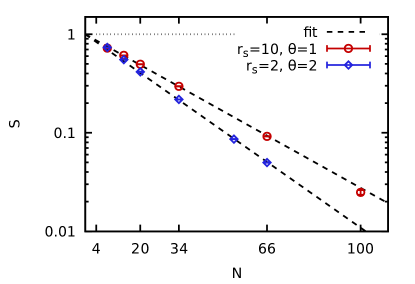
Figure 1: PIMC results for the average sign $S$ as a function of the system size $N$. The red circles and blue diamonds correspond to $r_{s}=10$, $\theta=1$ and $r_{s}=2$, $\theta=2$, respectively. The black dashed lines correspond to exponential fits according to Eq. (16) for $N\geq 20$. PIMC simulations are computationally feasible for $S\gtrsim 0.01$.

Let us start our investigation of the finite-size effects in the reconstructed PIMC results for the dynamic structure factor $S(q,\omega)$ by briefly touching upon the fermion sign problem within the PIMC simulations for both parameter combinations to be discussed in this work. To this end, we show our PIMC data for the average sign $S$ [i.e., the denominator of Eq. (4)] as a function of the system size $N$ in Fig. 1. Here the red circles and blue diamonds correspond to electron liquid and WDM conditions, respectively and exhibit a qualitatively similar behaviour. More specifically, the sign is strictly monotonically decreasing with $N$, and the dashed black lines depict exponential fits according to

$$S(N)=e^{-aN}\ ,$$ (16)

with $a$ being the free parameter. This is motivated by Eq. (5), and fits well to our PIMC data points for both cases. Furthermore, we note that the sign decays faster for the WDM case, which actually is a nontrivial finding. For higher densities (smaller values of $r_{s}$), electronic correlation effects become less important, and the particles are not that strongly separated. Consequently, fermionic exchange effects are more important, which results in a stronger amount of cancellations of positive and negative contributions, i.e., a decreasing average sign $S$. In this sense, the faster decrease of $S$ at $r_{s}=2$ surely is expected.

On the other hand, the electron liquid example has been obtained at half the value of the reduced temperature $\theta$. Let us for a moment consider the case of an ideal Fermi gas. In that case, the degree of quantum degeneracy, and, thus, the value of the corresponding average sign $S$ is fully defined by $\theta$ and does not depend on the density parameter $r_{s}$. Therefore, the sign for $r_{s}=10$ and $\theta=1$ would have been substantially lower compared to $r_{s}=2$ and $\theta=2$. Hence, the slower decay of $S$ in the red circles for the interacting case is purely a result of the increased Coulomb repulsion upon decreasing the density.

For completeness, we note that data with a sufficient accuracy for the reconstruction of $S(q,\omega)$ can be obtained for $S\gtrsim 0.1$ [resulting in a hundred-fold increase in computation time compared to bosons or boltzmannons, cf. Eq. (6)], i.e., $N\lesssim 54$ and $N\lesssim 66$ electrons for the WDM and electron liquid examples.

III.1 Warm dense matter regime: $r_{s}=2$ and $\theta=2$

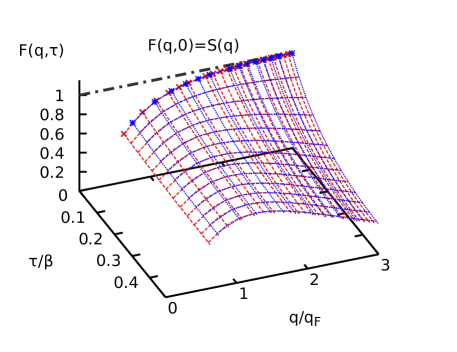
Figure 2: PIMC data for the imaginary-time density–density correlation function $F$ [cf. Eq. (7)] in the $\tau$-$x$-plane for $r_{s}=2$ and $\theta=2$. The red (dashed) and blue (dotted) data have been obtained for $N=34$ and $N=20$ electrons. Note that $F$ approaches the static structure factor in the $\tau=0$ limit (crosses and stars) and that it is symmetric with respect to $\tau=\beta/2$, i.e., $F(q,\tau)=F(q,\beta-\tau)$.

Due to the high current interest in the WDM regime, we will start our investigation of the system-size dependence of the dynamic structure factor at $r_{s}=2$ and $\theta=2$. However, before we consider $S(q,\omega)$ itself, it makes sense to first investigate any finite-size effects in the quantities that are used as input for the reconstruction. The imaginary-time density–density correlation function constitutes the most important ingredient and is depicted in Fig. 2 for $N=20$ (blue dotted) and $N=34$ (red dashed) unpolarized electrons in the $\tau$-$q$-plane. First and foremost, we note that a direct comparison between the two data sets is not possible, as $F$ is available at different $q$-points. This is an immediate consequence of the momentum quantization due to the finite box length $L$, see Refs. Dornheim et al. (2016b, 2017a) for a detailed explanation. The discretization in the $\tau$-direction, on the other hand, is defined by the selected number of imaginary-time propagators within a PIMC simulation, and can be chosen arbitrarily fine. In this work, we always use $P=200$ primitive propagators (see Refs. Brualla et al. (2004); Sakkos et al. (2009); Dornheim et al. (2019b) for a detailed and accessible discussion), which is sufficient to ensure convergence and allows for an adequate resolution with respect to the imaginary time $\tau$. We note that not all $\tau$-points are depicted in Fig. 2 to make it more accessible.

The red crosses and blue stars depict the $\tau\to 0$ limit of $F(q,\tau)$, which is given by the usual static structure factor

$$F(q,0)=S(q)=\int_{-\infty}^{\infty}\textnormal{d}\omega\ S(q,\omega)\ .$$ (17)

In other words, Eq. (17) means that the normalization of the reconstructed $S(q,\omega)$ (or, equivalently, $\braket{\omega^{0}}$) is known in advance.

Let us next come to the topic at hand, which is the dependence of $F(q,\tau)$ on the number of electrons $N$. Although no difference between the two particle numbers can be seen in Fig. 2, the depicted surface plot is not optimal for this purpose.

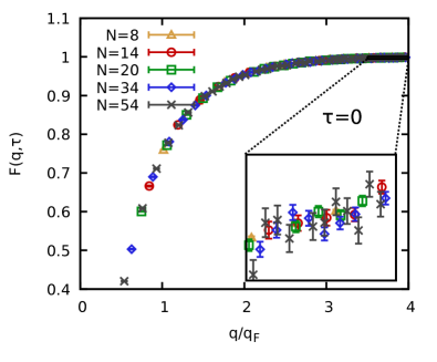
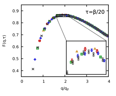
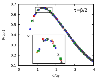
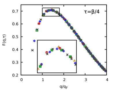
Figure 3: PIMC data for the imaginary-time density–density correlation function $F$ [cf. Eq. (7)] for $r_{s}=2$ and $\theta=2$. Shown is the $q$-dependence for different imaginary-time arguments, $\tau=0$ (i.e., $F(q,0)=S(q)$), $\tau=\beta/20$, $\tau=\beta/4$, and $\tau=\beta/2$ (clockwise). The different symbols correspond to $N=14,20,34,$ and $54$ electrons. The insets show magnified segments around the respective maxima.

A more systematic investigation is presented in Fig. 3, where we show $F(q,\tau)$ for four fixed values of the imaginary time along the $q$-direction. This has the advantage that we can directly compare PIMC results for different particle numbers, namely $N=8$ (yellow triangles), $N=14$ (red circles), $N=20$ (green squares), $N=34$ (blue diamonds), and $N=54$ (grey crosses). As a side note, we mention that it is fully sufficient to consider imaginary time values within the interval $\tau\in[0,\beta/2]$, as $F(q,\tau)$ is symmetric around $\beta/2$.

In the top left panel, we show results for $\tau=0$, i.e., for the usual static structure factor $S(q)$. At these conditions, there is not much spatial structure in the system, and $S(q)$ is a monotonically increasing function without any correlation-induced peaks. Moreover, the PIMC data for the different particle numbers are in excellent agreement over the entire depicted $q$-range, and no system-size dependence can be resolved within the given statistical uncertainty even for as few as $N=8$ electrons. While certainly being remarkable, this results is not unexpected, and similar observations have been reported both at finite temperature Dornheim et al. (2018a, 2017a, 2016b) and in the ground state Chiesa et al. (2006); Holzmann et al. (2016).

Moving on to $\tau=\beta/20$ (top right panel), the situation somewhat changes. Firstly, $F(q,\tau=\beta/20)$ is no longer monotonically increasing, but exhibits a maximum around twice the Fermi wave number $q_{\textnormal{F}}$. In addition, the results for $N=8$ are clearly shifted upward compared to the other particle numbers. A similar effect for $N=14$ is possible, but cannot be confirmed due to the given Monte-Carlo error bars, and all other data agree within the statistical uncertainty. For $\tau=\beta/4$ (bottom left panel) and $\tau=\beta/2$ (bottom right panel), we find the same trends regarding $N$ as for $\tau=\beta/20$, and the maximum is somewhat shifted towards smaller wave numbers with increasing $\tau$.

Based on this investigation of $F(q,\tau)$ alone, we would thus predict that the reconstructed spectra for $N\geq 20$ exhibit no finite-size effects, whereas they seem possible for $N=14$ and even likely for $N=20$.

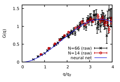
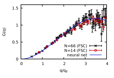
Figure 4: PIMC data for the $q$-dependence of the static local field correction $G(q)=G(q,0)$ for $r_{s}=2$ and $\theta=2+$. The black crosses and red circles depict simulation results for $N=66$ and $N=14$ electrons, and the blue curve has been obtained from the neural-net representation from Ref. Dornheim et al. (2019c). The left and right panels corresponds to the raw and finite-size corrected (FSC) PIMC data, respectively.

The second main ingredient to the reconstruction is the static limit of the LFC, i.e., $G(q)=\textnormal{Re}G(q,0)$, which can be readily computed from by solving Eq. (1) for $G$ after inserting the PIMC data for $\chi(q)$ that is obtained via Eq. (8). This procedure is explained in detail, e.g., in Refs. Dornheim et al. (2019c, 2020e). The results are shown in Fig. 4 for $N=14$ (red circles) and $N=66$ (grey crosses) electrons. Let us first focus on the left panel that has been directly obtained from the PIMC data for $\chi(q)$ without any additional finite-size correction. The solid blue line corresponds to the recent neural-net representation Dornheim et al. (2019c) of $G(q)$ and has been included as a guide to the eye. Evidently, all three curves exhibit a similar progression and can hardly be distinguished within the Monte-Carlo error bars. Yet, we note that the $N=66$ data points are in excellent agreement to the neural net, whereas the $N=14$ data appear to be somewhat too high for small wave numbers $q$.

The explanation is illustrated in the right panel, where the PIMC data for $G(q)$ have been finite-size corrected (see Ref. Groth et al. (2017b) for a detailed discussion of the finite-size correction of both $\chi(q)$ and $G(q)$). While the grey data set is hardly affected by this procedure, the red circles are shifted downwards towards the neural net representation. We thus note that finite-size effects in the static limit of the local field correction are quite small, but are noticeable in the case of $N\leq 14$ electrons.

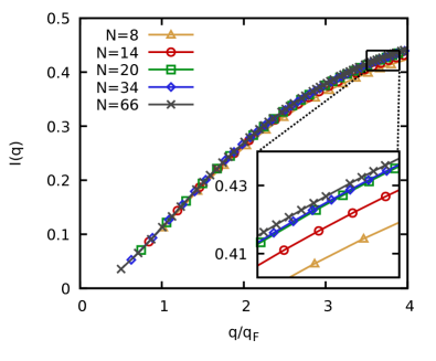
Figure 5: PIMC data for the $q$-dependence of the interaction function $I(q)$ [see Eq. (5)] for $r_{s}=2$ and $\theta=2$. The different symbols correspond to $N=8,14,20,34,$ and $66$ electrons and the inset shows a magnified segment for large $q$.

Let us conclude our analysis of the system-size dependence of the ingredients to the reconstruction procedure with an investigation of the high-frequency limit $G(q,\infty)=\textnormal{Re}G(q,\infty)$, which is defined in Eq. (12) in Sec. II.2. Apart from some trivial pre-factors, this limit is defined by a) the exchange–correlation contribution to the kinetic energy $K_{\textnormal{xc}}$ and b) the interaction integral Eq. (5) that depends on the static structure factor $S(q)$. Contribution a) is computed from the parametrization of the exchange–correlation free energy (in the thermodynamic limit) by Groth et al. Groth et al. (2017a), and, therefore, does not depend on the particle number $N$. The evaluation of contribution b), on the other hand, is nontrivial and deserves our attention.

Evidently, Eq. (5) requires to integrate the static structure factor $S(q)$ (or, to be precise, a function thereof) over continuous momenta $q$. This, however, is problematic as 1) PIMC data for $S(q)$ are only available for discrete $q$ values and 2) no PIMC data are available below a minimum value of $q_{\textnormal{min}}=2\pi/L$. In practice, we overcome this obstacle by performing cubic basis spline fits that combine the exact long-wavelength limit of $S(q)$ that is known from the perfect screening sum-rule Kugler (1970)

$$S_{0}(q)=\lim_{q\to 0}S(q)=\frac{q^{2}}{2\omega_{\textnormal{p}}}\textnormal{coth}\left(\frac{\beta\omega_{\textnormal{p}}}{2}\right)\ ,$$ (18)

with a smooth interpolation of the PIMC data elsewhere; see Ref. Dornheim et al. (2017a) for a detailed discussion of this procedure.

In Fig. 5, we show results for the interaction integral $I(q)$ that have been obtained by integrating the basis splines for different particle numbers. The behaviour with respect to $N$ is quite similar to $F(q,\tau)$ and we find noticeable finite-size effects for both $N=14$ and $N=8$, which increase towards large wave numbers.

Figure 6: Spline interpolation of the static structure factor. The solid yellow and dash-dotted green lines correspond to $S_{0}(q)$ [cf. Eq. (18)] and STLS. The red circles, blue diamonds, and dark grey crosses show PIMC results for $S(q)$ obtained for $N=14$, $N=34$, and $N=66$ electrons, respectively, and the corresponding curves cubic basis splines [see Ref. Dornheim et al. (2017a) for details] connecting $S_{0}(q)$ for small $q$ with the PIMC data elsewhere. Further, the vertical dashed grey line depicts the maximum $q$-value where $S_{0}(q)$ is used for $N=14$.

This can be understood by investigation the corresponding spline-fits of the static structure factor, which is shown in Fig. 6. The different symbols correspond to the $q$-values that are accessible in a PIMC simulation of $N=14$ (red circles), $N=34$ (blue diamonds), and $N=66$ (grey crosses) electrons, and the solid yellow curve to the exact long-wavelength behaviour of $S(q)$ that is given by Eq. (18). The corresponding spline representations of $S(q)$ have been obtained by combining the yellow curve up to an empirically chosen maximum $q$-value (cf. the vertical dashed grey line) with the PIMC data for a specific $N$ elsewhere. The dash-dotted green curve corresponds to the finite-temperature version Tanaka and Ichimaru (1986); Sjostrom and Dufty (2013) of the dielectric theory by Singwi et al. Singwi et al. (1968) and has been included as a reference. Evidently, the splines for $N=34$ and $N=66$ electrons cannot be distinguished over the entire depicted $q$-range, and the blue curve correctly predicts the data point for $S(q_{\textnormal{min}})$ for $N=66$ although it lies outside the fitting range. For $N=14$ (dotted red line), on the other hand, the range between $q_{\textnormal{min}}$ and the validity range of $S_{0}(q)$ is significantly larger, which makes the interpolation in between much less reliable. As a result, the red curve substantially deviates from the other two for $q\sim 0.5q_{\textnormal{F}}$, and this trend gets only more pronounced for $N=8$. The subsequent integration over these splines in Eq. (5) then leads to the finite-size effects in $I(q)$ observed in Fig. 5.

In a nutshell, we have found that the input data for the reconstruction procedure are afflicted with substantial finite-size errors for $N=8$ and noticeable errors for $N=14$ electrons.

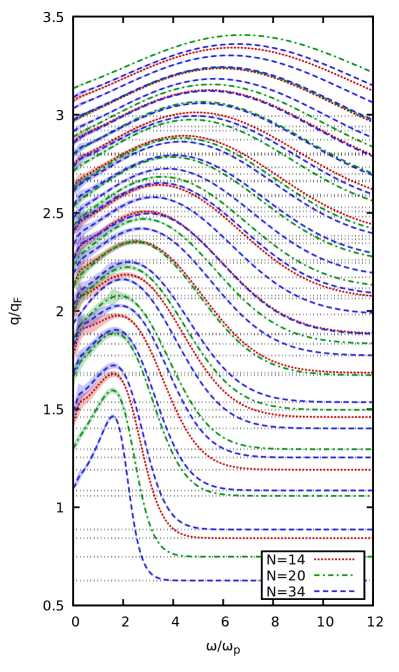
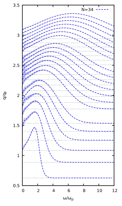
Figure 7: Reconstructed dynamic structure factors at WDM conditions ($r_{s}=2$ and $\theta=2$). Left panel: Solutions for $N=14$ (dotted red), $N=20$ (dash-dotted green), and $N=34$ (dashed blue) electrons at selected $q$-values. Right panel: Solutions for all $q$-values in the depicted $q$-range for $N=34$.

This brings us to the central topic of this work, which is the investigation of the system-size effects in the reconstructed dynamic structure factors $S(q,\omega)$ themselves. To this end, we show the full frequency-dependence of $S(q,\omega)$ for selected wave numbers in the left panel of Fig.7 for $N=14$ (red dotted), $N=20$ (dash-dotted green), and $N=34$ (dashed blue) electrons. For completeness, we note that it is sufficient to only show the positive $\omega$-range, since the DSF obeys the detailed balance relation Giuliani and Vignale (2008)

$$S(q,-\omega)=S(q,\omega)e^{-\beta\omega}\ .$$ (19)

Let us start by briefly touching upon the physical effects. In the limit of small wave numbers, the random phase approximation becomes exact and $S(q,\omega)$ becomes a delta-function around the plasma frequency $\omega_{\textnormal{p}}=\sqrt{3/r_{s}^{3}}$. With increasing $q$, the DSF broadens in the frequency domain, and the normalization [i.e., the static structure factor $S(q)$, cf. Eq. (17)] increases until it saturates around one. Here, too, the random phase approximation becomes exact, as the impact of the local field correction is reduced by the $4\pi/q^{2}$ pre-factor, cf. Eq. (1).

Regarding the reconstructed solutions for $S(q,\omega)$ for different $S(q,\omega)$, we find that the subsequent curves exhibit a smooth progression in the $q$-$\omega$-plane, and even the results for $N=14$ electrons do not exhibit any noticeable deviations from this trend. While only certain wave numbers are included in this plot, we show the full dispersion relation of all $q$-values in the depicted wave number range for $N=34$ electrons in the right panel of Fig. 7. A common feature of both panels is given by the increased uncertainty for small frequencies, which is consistent with the previous findings from Refs. Dornheim et al. (2018b); Groth et al. (2019) in this regime. In principle, this would allow for the possibility of a diffusive feature for small $\omega$ (see, e.g., Ref. Vorberger et al. (2012)), but this is not expected for the present case of a quantum one-component system.

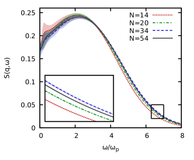
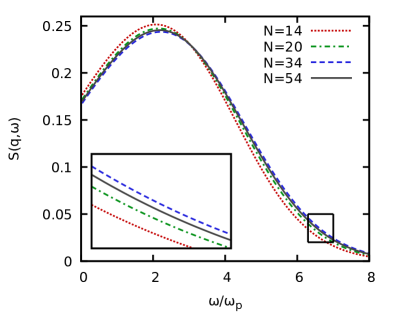
Figure 8: Dynamic structure factor of the UEG at $r_{s}=2$ and $\theta=2$. The dotted red, dash-dotted green, dashed blue and solid black lines correspond to $N=14$ ($q/q_{\textnormal{F}}\approx 1.460$), $N=20$ ($q/q_{\textnormal{F}}\approx 1.496$), $N=34$ ($q/q_{\textnormal{F}}\approx 1.536$), and $N=54$ ($q/q_{\textnormal{F}}\approx 1.520$) electrons, where the numbers in brackets indicate the respective wave number $q$. The left panel shows the full reconstructed solutions for $S(q,\omega)$, and the right panel the corresponding curves from the static approximation that has been included as a reference.

In order to more rigorously discard the possibility of finite-size effects in our data for the DSF, we show $S(q,\omega)$ for similar wave numbers around $q=1.5q_{\textnormal{F}}$ in the left panel of Fig. 8 for $N=14$ (dotted red), $N=20$ (dash-dotted green), $N=34$ (dashed blue), and $N=54$ (solid grey). First and foremost, we note that all curves exhibit a very similar behaviour over the entire $\omega$-range. Yet, while the curves agree within the given confidence interval for $\omega\lesssim 3\omega_{\textnormal{p}}$, there appear systematic deviations for larger frequencies. In principle, these could be 1) due to finite-size effects, 2) inconsistencies in the reconstruction procedure that are not accounted for by the confidence interval [cf. Eq. 15)], or 3) due to the different $q$-values for the four cases, see the caption.

To resolve this issue, we compute the same curves within the so-called static approximation, i.e., by inserting the exact static limit $G(q,0)$ into Eq. (1) to get $\chi_{\textnormal{static}}(q,\omega)$ and subsequently evoking the fluctuation–dissipation theorem [Eq. (11)] to compute the corresponding DSF $S_{\textnormal{static}}(q,\omega)$. The results are shown in the right panel of Fig. 8, and exhibit precisely the same order as the fully reconstructed curves in the left panel. For instance, the insets of both panels depict magnified segments for the large-$\omega$ regime, and, the curves are ordered with decreasing wave number starting from the top.

We thus conclude that the observed differences are due to explanation 3), and no finite-size effects can be resolved in the reconstructed solution for $S(q,\omega)$ even for as few as $N=14$ electrons.

In contrast, for $N=8$ our reconstruction procedure was not able to find viable solutions for $S(q,\omega)$ which were then in agreement to the PIMC data for $F(q,\tau)$ and $\braket{\omega^{k}}$. This means that finite-size effects do not manifest as an $N$-dependence in the reconstructed spectra, but as an inconsistency between the exact constraints on $G(q,\omega)$ (cf. Sec. II.2) and the potentially system-size dependent PIMC data.

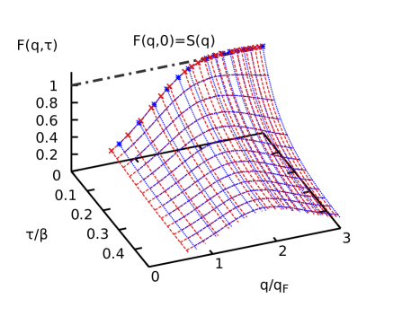
Figure 9: PIMC data for the imaginary-time density–density correlation function $F$ [cf. Eq. (7)] in the $\tau$-$x$-plane for $r_{s}=10$ and $\theta=1$. The red (dashed) and blue (dotted) data have been obtained for $N=34$ and $N=20$ electrons. Note that $F$ approaches the static structure factor in the $\tau=0$ limit (crosses and stars) and that it is symmetric with respect to $\tau=\beta/2$, i.e., $F(q,\tau)=F(q,\beta-\tau)$.

III.2 Strongly correlated regime: $r_{s}=10$ and $\theta=1$

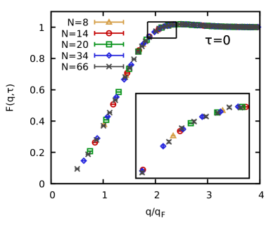
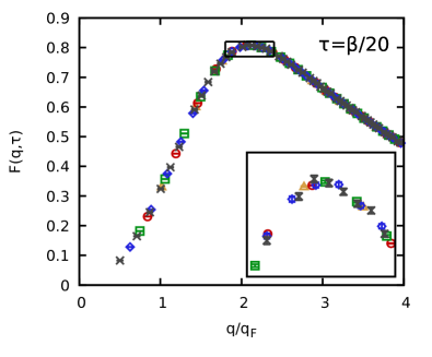
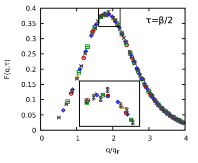
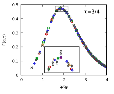
Figure 10: PIMC data for the imaginary-time density–density correlation function $F$ [cf. Eq. (7)] for $r_{s}=10$ and $\theta=1$. Shown is the $q$-dependence for different imaginary-time arguments, $\tau=0$ (i.e., $F(q,0)=S(q)$), $\tau=\beta/20$, $\tau=\beta/4$, and $\tau=\beta/2$ (clockwise). The different symbols correspond to $N=8,14,20,34,$ and $66$ electrons. The insets show magnified segments around the respective maxima.

The second parameter regime to be explored in this work is given by the margins of the electron liquid ($r_{s}=10$ and $\theta=1$). Despite being less relevant for current WDM experiments, these conditions offer a plethora of interesting physical effects. Of particular relevance is a possible incipient excitonic mode that was predicted by Takada Takada (2016) (see also Ref. Higuchi and Yasuhara (2000) for a discussion of the excitonic nature of this feature) and substantiated by Dornheim et al. Dornheim et al. (2018b). Further, we mention that this regime is particularly interesting from a theoretical perspective, as the full frequency-dependence of $G(q,\omega)$ is needed for an adequate description. This is in stark contrast to the WDM regime, where using the static limit $G(q,0)$ is often sufficient to obtain highly accurate results for all $\omega$.

Since this analysis is mostly analogous to the discussion of WDM parameters in the previous section, here we only briefly state the most important findings. In Fig. 9, we show the imaginary-time density–density correlation function in the $q$-$\tau$-plane again for $N=20$ (blue) and $N=34$ (red) unpolarized electrons. In contrast to the WDM example shown in Fig. 2, here $F(q,\tau)$ exhibits a more complicated structure, and the static structure factor $S(q)=F(q,0)$ has a small maximum around twice the Fermi wave number and is thus non monotonous. Although, in general, the direct physical interpretation of this quantity is rather difficult, it was found that the amount of structure substantially increases with coupling strength, with a progression of several maxima and minima in the electron liquid regime Dornheim et al. (2020d). Still, no difference between the two system sizes can be spotted in Fig. 9.

A more detailed investigation is presented in Fig. 10, where we show the $q$-dependence of $F$ for fixed $\tau$-values. Interestingly, no finite size effects are evident anywhere even for as few as $N=8$ electrons. This is not fully unexpected, as the system size dependence is known to increase both with density and with temperature Dornheim et al. (2016b) at these conditions. For completeness, we mention that for even lower temperatures ($\theta\lesssim 0.25$), shell-filling effects in momentum-space become important that can be mitigated by simulating commensurate particle numbers (i.e., $N=33$ or $N=66$ electrons for a spin-polarized or unpolarized system) and by carrying out an additional twist-averaging procedure Lin et al. (2001); Spink et al. (2013).

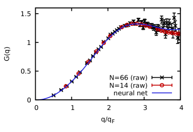
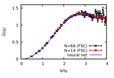
Figure 11: PIMC data for the $q$-dependence of the static local field correction $G(q)=G(q,0)$ for $r_{s}=10$ and $\theta=1$. The black crosses and red circles depict simulation results for $N=66$ and $N=14$ electrons, and the blue curve has been obtained from the neural-net representation from Ref. Dornheim et al. (2019c). The left and right panels corresponds to the raw and finite-size corrected (FSC) PIMC data, respectively.

The next relevant input quantity to the reconstruction procedure is given by the static limit of $G(q,\omega)$, which is shown in Fig. 11. Again, even for $N=14$ electrons almost no finite-size effects are visible in the pure PIMC data (left panel), and the finite-size correction (right panel) only affects the data for $q\gtrsim 3q_{\textnormal{F}}$.

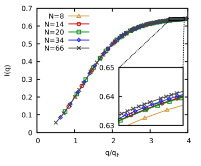
Figure 12: PIMC data for the $q$-dependence of the interaction function $I(q)$ [cf. Eq. (7)] for $r_{s}=10$ and $\theta=1$. The different symbols correspond to $N=8,14,20,34,$ and $66$ electrons and the inset shows a magnified segment for large $q$.

Finally, we show results for the interaction integral $I(q)$ [cf. Eq. (5)] in Fig. 12. In contrast to $F(q,\tau)$, here there do appear some differences between $N=8$ (yellow triangles) and the other curves. We thus conclude that there should be no finite-size effects in the reconstructed dynamic structure factors except possibly for $N=8$.

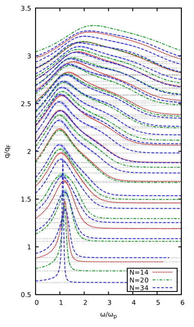
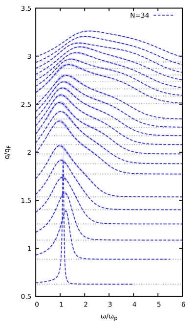
Figure 13: Fully reconstructed dynamic structure factor of the UEG at $r_{s}=10$ and $\theta=1$ for selected wave numbers. The dashed red, dash-dotted green, dashed blue, and solid black curves have been obtained for $N=14$, $N=20$, and $N=34$ electrons, respectively.

Let us conclude this study with an analysis of $S(q,\omega)$ itself, which is shown in the $q$-$\omega$-plane for selected wave numbers in the left panel of Fig. 13 for $N=14$ (dotted red), $N=20$ (dash-dotted green), and $N=34$ (dashed blue) electrons. Due to the reduced density and the lower temperature compared to the WDM dispersion shown in Fig. 7, the curve for the smallest $q$-value for $N=34$ exhibits a rather sharp peak that is only slightly shifted away from the plasma frequency. In this context, we remark that our reconstruction scheme has no problem with such distinct features, which is in stark contrast to other inversion methods where the obtained spectra are often artificially broadened. Furthermore, we have obtained the familiar dispersion with the superposition of a mean-field contribution around $\omega_{\textnormal{mf}}=q^{2}/2+\omega_{\textnormal{p}}$ and an additional incipient mode at lower frequencies that has been reported in Ref. Dornheim et al. (2018b).

Yet, the important point for the present investigation is that no systematic finite-size effects occur between the curves for different $N$ at subsequent wave numbers. For completeness, we note that there do occur some small variation for some larger wave numbers, these are an artifact of the reconstruction procedure itself and not related to $N$. To verify this claim, we also show the full dispersion relation (i.e., all $q$-values in the depicted wave-number range) in the right panel of Fig. 13. Here, one can clearly see that the dynamic structure factor for the third-largest $q$-value is somewhat inconsistent to the other curves, although the system size is the same everywhere.

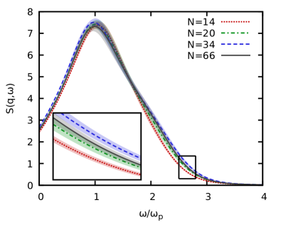
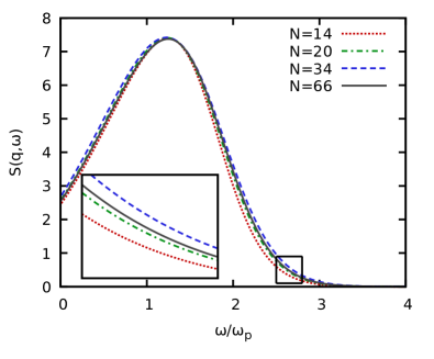
Figure 14: Dynamic structure factor of the UEG at $r_{s}=10$ and $\theta=1$. The dotted red, dash-dotted green, dashed blue and solid black lines correspond to $N=14$ ($q/q_{\textnormal{F}}\approx 1.460$), $N=20$ ($q/q_{\textnormal{F}}\approx 1.496$), $N=34$ ($q/q_{\textnormal{F}}\approx 1.536$), and $N=66$ ($q/q_{\textnormal{F}}\approx 1.508$) electrons, where the numbers in brackets indicate the respective wave number $q$. The left panel shows the full reconstructed solutions for $S(q,\omega)$, and the right panel the corresponding curves from the static approximation that has been included as a reference.

The lack of finite-size effects in the dynamic structure factor can also be seen even more clearly in Fig. 14, where $S(q,\omega)$ is shown for different particle numbers at similar wave numbers around $q=1.5q_{\textnormal{F}}$. The left panel shows the reconstructed solutions [i.e., using the full frequency dependence of $G(q,\omega)$] and, similar to the WDM example depicted in Fig. 8, only minor differences occur, mainly for large frequencies. Again, these small deviations are fully explained by the slightly different $q$-values for the four curves, and completely reproduced by the static approximation shown in the right panel, see also Sec. III.1 for a more detailed discussion.

Finally, we mention that here, too, no consistent solutions could be found for $N=8$, which further substantiates our previous finding from the WDM regime that finite-size effects manifest not in an $N$-dependence of $S(q,\omega)$ itself, but in the impossibility to match the exact constraints on $G(q,\omega)$ [cf. Sec. II.2] with the PIMC data.

IV Summary and Outlook

In this work, we have investigated in detail the possibility of finite-size effects in the dynamic structure factor of the uniform electron gas both at WDM conditions, and at the margins of the strongly coupled electron liquid regime. More specifically, $S(q,\omega)$ can be accurately reconstructed on the basis of ab initio PIMC data, which, while being exact with respect to exchange–correlation effects, have been obtained for a finite simulation cell. In a nut shell, we have found that even as few $N=14$ electrons are sufficient to give accurate results for $S(q,\omega)$ that are converged with respect to $N$, and no system-size dependence could be resolved within the given confidence level. In contrast, no solutions for $S(q,\omega)$ could be found for $N=8$ electrons, as the exact constraints on the dynamic local field correction $G(q,\omega)$ that are incorporated into the reconstruction procedure cannot be matched to the PIMC data when the latter are not converged with respect to $N$.

Therefore, the current analysis further corroborates the high quality of the electronic structure factors presented in Refs. Dornheim et al. (2018b); Groth et al. (2019). This is an important finding, as the dynamic density response is of key relevance for many applications (see Sec. I) like the construction of dynamic exchange–correlation kernels for time-dependent DFT simulations Baczewski et al. (2016) or the ongoing investigation of the incipient excitonic mode in the UEG Dornheim et al. (2018b).

References

References

- Fortov (2009) V. E. Fortov, “Extreme states of matter on earth and in space,” Phys.-Usp 52, 615–647 (2009).
- Graziani et al. (2014) F. Graziani, M. P. Desjarlais, R. Redmer, and S. B. Trickey, eds., Frontiers and Challenges in Warm Dense Matter (Springer, International Publishing, 2014).
- Saumon et al. (1992) D. Saumon, W. B. Hubbard, G. Chabrier, and H. M. van Horn, “The role of the molecular-metallic transition of hydrogen in the evolution of jupiter, saturn, and brown dwarfs,” Astrophys. J 391, 827–831 (1992).
- Militzer et al. (2008) B. Militzer, W. B. Hubbard, J. Vorberger, I. Tamblyn, and S. A. Bonev, “A massive core in jupiter predicted from first-principles simulations,” The Astrophysical Journal 688, L45–L48 (2008).
- Guillot et al. (2018) T. Guillot, Y. Miguel, B. Militzer, W. B. Hubbard, Y. Kaspi, E. Galanti, H. Cao, R. Helled, S. M. Wahl, L. Iess, W. M. Folkner, D. J. Stevenson, J. I. Lunine, D. R. Reese, A. Biekman, M. Parisi, D. Durante, J. E. P. Connerney, S. M. Levin, and S. J. Bolton, “A suppression of differential rotation in jupiter’s deep interior,” Nature 555, 227–230 (2018).
- Becker et al. (2014) A. Becker, W. Lorenzen, J. J. Fortney, N. Nettelmann, M. Schöttler, and R. Redmer, “Ab initio equations of state for hydrogen (h-reos.3) and helium (he-reos.3) and their implications for the interior of brown dwarfs,” Astrophys. J. Suppl. Ser 215, 21 (2014).
- Hu et al. (2011) S. X. Hu, B. Militzer, V. N. Goncharov, and S. Skupsky, “First-principles equation-of-state table of deuterium for inertial confinement fusion applications,” Phys. Rev. B 84, 224109 (2011).
- Moses et al. (2009) E. I. Moses, R. N. Boyd, B. A. Remington, C. J. Keane, and R. Al-Ayat, “The national ignition facility: Ushering in a new age for high energy density science,” Physics of Plasmas 16, 041006 (2009), https://doi.org/10.1063/1.3116505 .
- Bostedt et al. (2016) Christoph Bostedt, Sébastien Boutet, David M. Fritz, Zhirong Huang, Hae Ja Lee, Henrik T. Lemke, Aymeric Robert, William F. Schlotter, Joshua J. Turner, and Garth J. Williams, “Linac coherent light source: The first five years,” Rev. Mod. Phys. 88, 015007 (2016).
- Tschentscher et al. (2017) Thomas Tschentscher, Christian Bressler, Jan Grünert, Anders Madsen, Adrian P. Mancuso, Michael Meyer, Andreas Scherz, Harald Sinn, and Ulf Zastrau, “Photon beam transport and scientific instruments at the european xfel,” Applied Sciences 7 (2017), 10.3390/app7060592.
- Falk (2018) K. Falk, “Experimental methods for warm dense matter research,” High Power Laser Sci. Eng 6, e59 (2018).
- Kraus et al. (2016) D. Kraus, A. Ravasio, M. Gauthier, D. O. Gericke, J. Vorberger, S. Frydrych, J. Helfrich, L. B. Fletcher, G. Schaumann, B. Nagler, B. Barbrel, B. Bachmann, E. J. Gamboa, S. Göde, E. Granados, G. Gregori, H. J. Lee, P. Neumayer, W. Schumaker, T. Döppner, R. W. Falcone, S. H. Glenzer, and M. Roth, “Nanosecond formation of diamond and lonsdaleite by shock compression of graphite,” Nature Communications 7, 10970 (2016).
- Kraus et al. (2017) D. Kraus, J. Vorberger, A. Pak, N. J. Hartley, L. B. Fletcher, S. Frydrych, E. Galtier, E. J. Gamboa, D. O. Gericke, S. H. Glenzer, E. Granados, M. J. MacDonald, A. J. MacKinnon, E. E. McBride, I. Nam, P. Neumayer, M. Roth, A. M. Saunders, A. K. Schuster, P. Sun, T. van Driel, T. Döppner, and R. W. Falcone, “Formation of diamonds in laser-compressed hydrocarbons at planetary interior conditions,” Nature Astronomy 1, 606–611 (2017).
- Kritcher et al. (2008) Andrea L. Kritcher, Paul Neumayer, John Castor, Tilo Döppner, Roger W. Falcone, Otto L. Landen, Hae Ja Lee, Richard W. Lee, Edward C. Morse, Andrew Ng, Steve Pollaine, Dwight Price, and Siegfried H. Glenzer, “Ultrafast x-ray thomson scattering of shock-compressed matter,” Science 322, 69–71 (2008), https://science.sciencemag.org/content/322/5898/69.full.pdf .
- Mo et al. (2018) M. Z. Mo, Z. Chen, R. K. Li, M. Dunning, B. B. L. Witte, J. K. Baldwin, L. B. Fletcher, J. B. Kim, A. Ng, R. Redmer, A. H. Reid, P. Shekhar, X. Z. Shen, M. Shen, K. Sokolowski-Tinten, Y. Y. Tsui, Y. Q. Wang, Q. Zheng, X. J. Wang, and S. H. Glenzer, “Heterogeneous to homogeneous melting transition visualized with ultrafast electron diffraction,” Science 360, 1451–1455 (2018), https://science.sciencemag.org/content/360/6396/1451.full.pdf .
- Bonitz et al. (2020) M. Bonitz, T. Dornheim, Zh. A. Moldabekov, S. Zhang, P. Hamann, H. Kählert, A. Filinov, K. Ramakrishna, and J. Vorberger, “Ab initio simulation of warm dense matter,” Physics of Plasmas 27, 042710 (2020), https://doi.org/10.1063/1.5143225 .
- Dornheim et al. (2018a) T. Dornheim, S. Groth, and M. Bonitz, “The uniform electron gas at warm dense matter conditions,” Phys. Reports 744, 1–86 (2018a).
- Ceperley (1995) D. M. Ceperley, “Path integrals in the theory of condensed helium,” Rev. Mod. Phys 67, 279 (1995).
- Takahashi and Imada (1984) Minoru Takahashi and Masatoshi Imada, “Monte carlo calculation of quantum systems,” Journal of the Physical Society of Japan 53, 963–974 (1984).
- Herman et al. (1982) M. F. Herman, E. J. Bruskin, and B. J. Berne, “On path integral monte carlo simulations,” The Journal of Chemical Physics 76, 5150–5155 (1982), https://doi.org/10.1063/1.442815 .
- Troyer and Wiese (2005) M. Troyer and U. J. Wiese, “Computational complexity and fundamental limitations to fermionic quantum Monte Carlo simulations,” Phys. Rev. Lett 94, 170201 (2005).
- Dornheim (2019) T. Dornheim, “Fermion sign problem in path integral Monte Carlo simulations: Quantum dots, ultracold atoms, and warm dense matter,” Phys. Rev. E 100, 023307 (2019).
- Dornheim et al. (2019a) T. Dornheim, S. Groth, A. V. Filinov, and M. Bonitz, “Path integral monte carlo simulation of degenerate electrons: Permutation-cycle properties,” The Journal of Chemical Physics 151, 014108 (2019a), https://doi.org/10.1063/1.5093171 .
- Driver and Militzer (2012) K. P. Driver and B. Militzer, “All-electron path integral monte carlo simulations of warm dense matter: Application to water and carbon plasmas,” Phys. Rev. Lett. 108, 115502 (2012).
- Brown et al. (2013) Ethan W. Brown, Bryan K. Clark, Jonathan L. DuBois, and David M. Ceperley, “Path-integral monte carlo simulation of the warm dense homogeneous electron gas,” Phys. Rev. Lett. 110, 146405 (2013).
- Blunt et al. (2014) N. S. Blunt, T. W. Rogers, J. S. Spencer, and W. M. C. Foulkes, “Density-matrix quantum monte carlo method,” Phys. Rev. B 89, 245124 (2014).
- Schoof et al. (2015) T. Schoof, S. Groth, J. Vorberger, and M. Bonitz, “Ab initio thermodynamic results for the degenerate electron gas at finite temperature,” Phys. Rev. Lett. 115, 130402 (2015).
- Filinov et al. (2015) V. S. Filinov, V. E. Fortov, M. Bonitz, and Zh. Moldabekov, “Fermionic path-integral monte carlo results for the uniform electron gas at finite temperature,” Phys. Rev. E 91, 033108 (2015).
- Chin (2015) Siu A. Chin, “High-order path-integral monte carlo methods for solving quantum dot problems,” Phys. Rev. E 91, 031301 (2015).
- Dornheim et al. (2015a) Tobias Dornheim, Simon Groth, Alexey Filinov, and Michael Bonitz, “Permutation blocking path integral monte carlo: a highly efficient approach to the simulation of strongly degenerate non-ideal fermions,” New Journal of Physics 17, 073017 (2015a).
- Dornheim et al. (2015b) Tobias Dornheim, Tim Schoof, Simon Groth, Alexey Filinov, and Michael Bonitz, “Permutation blocking path integral monte carlo approach to the uniform electron gas at finite temperature,” The Journal of Chemical Physics 143, 204101 (2015b), https://doi.org/10.1063/1.4936145 .
- Militzer and Driver (2015) Burkhard Militzer and Kevin P. Driver, “Development of path integral monte carlo simulations with localized nodal surfaces for second-row elements,” Phys. Rev. Lett. 115, 176403 (2015).
- Malone et al. (2015) Fionn D. Malone, N. S. Blunt, James J. Shepherd, D. K. K. Lee, J. S. Spencer, and W. M. C. Foulkes, “Interaction picture density matrix quantum monte carlo,” The Journal of Chemical Physics 143, 044116 (2015), https://doi.org/10.1063/1.4927434 .
- Groth et al. (2016) S. Groth, T. Schoof, T. Dornheim, and M. Bonitz, “Ab initio quantum monte carlo simulations of the uniform electron gas without fixed nodes,” Phys. Rev. B 93, 085102 (2016).
- Dornheim et al. (2016a) T. Dornheim, S. Groth, T. Schoof, C. Hann, and M. Bonitz, “Ab initio quantum monte carlo simulations of the uniform electron gas without fixed nodes: The unpolarized case,” Phys. Rev. B 93, 205134 (2016a).
- Malone et al. (2016) Fionn D. Malone, N. S. Blunt, Ethan W. Brown, D. K. K. Lee, J. S. Spencer, W. M. C. Foulkes, and James J. Shepherd, “Accurate exchange-correlation energies for the warm dense electron gas,” Phys. Rev. Lett. 117, 115701 (2016).
- Dornheim et al. (2016b) T. Dornheim, S. Groth, T. Sjostrom, F. D. Malone, W. M. C. Foulkes, and M. Bonitz, “Ab initio quantum Monte Carlo simulation of the warm dense electron gas in the thermodynamic limit,” Phys. Rev. Lett. 117, 156403 (2016b).
- Dornheim et al. (2017a) T. Dornheim, S. Groth, and M. Bonitz, “Ab initio results for the static structure factor of the warm dense electron gas,” Contrib. Plasma Phys 57, 468–478 (2017a).
- Groth et al. (2017a) S. Groth, T. Dornheim, T. Sjostrom, F. D. Malone, W. M. C. Foulkes, and M. Bonitz, “Ab initio exchange–correlation free energy of the uniform electron gas at warm dense matter conditions,” Phys. Rev. Lett. 119, 135001 (2017a).
- Claes and Clark (2017) Jahan Claes and Bryan K. Clark, “Finite-temperature properties of strongly correlated systems via variational monte carlo,” Phys. Rev. B 95, 205109 (2017).
- Dornheim et al. (2017b) Tobias Dornheim, Simon Groth, Fionn D. Malone, Tim Schoof, Travis Sjostrom, W. M. C. Foulkes, and Michael Bonitz, “Ab initio quantum monte carlo simulation of the warm dense electron gas,” Physics of Plasmas 24, 056303 (2017b), https://doi.org/10.1063/1.4977920 .
- Liu et al. (2018) Yuan Liu, Minsik Cho, and Brenda Rubenstein, “Ab initio finite temperature auxiliary field quantum monte carlo,” Journal of Chemical Theory and Computation 14, 4722–4732 (2018).
- Dornheim et al. (2019b) Tobias Dornheim, Simon Groth, and Michael Bonitz, “Permutation blocking path integral monte carlo simulations of degenerate electrons at finite temperature,” Contributions to Plasma Physics 59, e201800157 (2019b), https://onlinelibrary.wiley.com/doi/pdf/10.1002/ctpp.201800157 .
- Spencer et al. (2019) James S. Spencer, Nick S. Blunt, Seonghoon Choi, Jiří Etrych, Maria-Andreea Filip, W. M. C. Foulkes, Ruth S. T. Franklin, Will J. Handley, Fionn D. Malone, Verena A. Neufeld, Roberto Di Remigio, Thomas W. Rogers, Charles J. C. Scott, James J. Shepherd, William A. Vigor, Joseph Weston, RuQing Xu, and Alex J. W. Thom, “The hande-qmc project: Open-source stochastic quantum chemistry from the ground state up,” Journal of Chemical Theory and Computation 15, 1728–1742 (2019).
- Hirshberg et al. (2020) Barak Hirshberg, Michele Invernizzi, and Michele Parrinello, “Path integral molecular dynamics for fermions: Alleviating the sign problem with the bogoliubov inequality,” The Journal of Chemical Physics 152, 171102 (2020), https://doi.org/10.1063/5.0008720 .
- Dornheim et al. (2020a) Tobias Dornheim, Jan Vorberger, and Michael Bonitz, “Nonlinear electronic density response in warm dense matter,” Phys. Rev. Lett. 125, 085001 (2020a).
- Yilmaz et al. (2020) A. Yilmaz, K. Hunger, T. Dornheim, S. Groth, and M. Bonitz, “Restricted configuration path integral monte carlo,” The Journal of Chemical Physics 153, 124114 (2020), https://doi.org/10.1063/5.0022800 .
- Dornheim et al. (2020b) Tobias Dornheim, Michele Invernizzi, Jan Vorberger, and Barak Hirshberg, “Attenuating the fermion sign problem in path integral monte carlo simulations using the bogoliubov inequality and thermodynamic integration,” (2020b), arXiv:2009.11036 [physics.comp-ph] .
- Karasiev et al. (2014) Valentin V. Karasiev, Travis Sjostrom, James Dufty, and S. B. Trickey, “Accurate homogeneous electron gas exchange-correlation free energy for local spin-density calculations,” Phys. Rev. Lett. 112, 076403 (2014).
- Ceperley and Alder (1980) D. M. Ceperley and B. J. Alder, “Ground state of the electron gas by a stochastic method,” Phys. Rev. Lett. 45, 566–569 (1980).
- Vosko et al. (1980) S. H. Vosko, L. Wilk, and M. Nusair, “Accurate spin-dependent electron liquid correlation energies for local spin density calculations: a critical analysis,” Canadian Journal of Physics 58, 1200–1211 (1980), https://doi.org/10.1139/p80-159 .
- Perdew and Zunger (1981) J. P. Perdew and Alex Zunger, “Self-interaction correction to density-functional approximations for many-electron systems,” Phys. Rev. B 23, 5048–5079 (1981).
- Sjostrom and Daligault (2014) Travis Sjostrom and Jérôme Daligault, “Gradient corrections to the exchange-correlation free energy,” Phys. Rev. B 90, 155109 (2014).
- Karasiev et al. (2016) V. V. Karasiev, L. Calderin, and S. B. Trickey, “Importance of finite-temperature exchange correlation for warm dense matter calculations,” Phys. Rev. E 93, 063207 (2016).
- Ramakrishna et al. (2020) Kushal Ramakrishna, Tobias Dornheim, and Jan Vorberger, “Influence of finite temperature exchange-correlation effects in hydrogen,” Phys. Rev. B 101, 195129 (2020).
- Giuliani and Vignale (2008) G. Giuliani and G. Vignale, Quantum Theory of the Electron Liquid (Cambridge University Press, Cambridge, 2008).
- Kugler (1975) A. A. Kugler, “Theory of the local field correction in an electron gas,” J. Stat. Phys 12, 35 (1975).
- Lu (2014) Deyu Lu, “Evaluation of model exchange-correlation kernels in the adiabatic connection fluctuation-dissipation theorem for inhomogeneous systems,” The Journal of Chemical Physics 140, 18A520 (2014), https://doi.org/10.1063/1.4867538 .
- Patrick and Thygesen (2015) Christopher E. Patrick and Kristian S. Thygesen, “Adiabatic-connection fluctuation-dissipation dft for the structural properties of solids—the renormalized alda and electron gas kernels,” The Journal of Chemical Physics 143, 102802 (2015), https://doi.org/10.1063/1.4919236 .
- Pribram-Jones et al. (2016) Aurora Pribram-Jones, Paul E. Grabowski, and Kieron Burke, “Thermal density functional theory: Time-dependent linear response and approximate functionals from the fluctuation-dissipation theorem,” Phys. Rev. Lett. 116, 233001 (2016).
- Görling (2019) Andreas Görling, “Hierarchies of methods towards the exact kohn-sham correlation energy based on the adiabatic-connection fluctuation-dissipation theorem,” Phys. Rev. B 99, 235120 (2019).
- Baczewski et al. (2016) A. D. Baczewski, L. Shulenburger, M. P. Desjarlais, S. B. Hansen, and R. J. Magyar, “X-ray thomson scattering in warm dense matter without the chihara decomposition,” Phys. Rev. Lett 116, 115004 (2016).
- Moldabekov et al. (2018a) Zh. A. Moldabekov, M. Bonitz, and T. S. Ramazanov, “Theoretical foundations of quantum hydrodynamics for plasmas,” Physics of Plasmas 25, 031903 (2018a), https://doi.org/10.1063/1.5003910 .
- Diaw and Murillo (2015) A. Diaw and M. S. Murillo, “Generalized hydrodynamics model for strongly coupled plasmas,” Phys. Rev. E 92, 013107 (2015).
- Diaw and Murillo (2017) Abdourahmane Diaw and Michael S. Murillo, “A viscous quantum hydrodynamics model based on dynamic density functional theory,” Scientific Reports 7, 15352 (2017).
- Senatore et al. (1996) G. Senatore, S. Moroni, and D. M. Ceperley, “Local field factor and effective potentials in liquid metals,” J. Non-Cryst. Sol 205-207, 851–854 (1996).
- Moldabekov et al. (2018b) Zh.A. Moldabekov, S. Groth, T. Dornheim, H. Kählert, M. Bonitz, and T. S. Ramazanov, “Structural characteristics of strongly coupled ions in a dense quantum plasma,” Phys. Rev. E 98, 023207 (2018b).
- Moldabekov et al. (2019) Zh.A. Moldabekov, H. Kählert, T. Dornheim, S. Groth, M. Bonitz, and T. S. Ramazanov, “Dynamical structure factor of strongly coupled ions in a dense quantum plasma,” Phys. Rev. E 99, 053203 (2019).
- Veysman et al. (2016) M. Veysman, G. Röpke, M. Winkel, and H. Reinholz, “Optical conductivity of warm dense matter within a wide frequency range using quantum statistical and kinetic approaches,” Phys. Rev. E 94, 013203 (2016).
- Desjarlais et al. (2017) Michael P. Desjarlais, Christian R. Scullard, Lorin X. Benedict, Heather D. Whitley, and Ronald Redmer, “Density-functional calculations of transport properties in the nondegenerate limit and the role of electron-electron scattering,” Phys. Rev. E 95, 033203 (2017).
- Moldabekov et al. (2020) Zh. A. Moldabekov, T. Dornheim, M. Bonitz, and T. S. Ramazanov, “Ion energy-loss characteristics and friction in a free-electron gas at warm dense matter and nonideal dense plasma conditions,” Phys. Rev. E 101, 053203 (2020).
- Vorberger et al. (2010) J. Vorberger, D. O. Gericke, Th. Bornath, and M. Schlanges, “Energy relaxation in dense, strongly coupled two-temperature plasmas,” Phys. Rev. E 81, 046404 (2010).
- Benedict et al. (2017) L. X. Benedict, M. P. Surh, L. G. Stanton, C. R. Scullard, A. A. Correa, J. I. Castor, F. R. Graziani, L. A. Collins, O. Certík, J. D. Kress, and M. S. Murillo, “Molecular dynamics studies of electron-ion temperature equilibration in hydrogen plasmas within the coupled-mode regime,” Phys. Rev. E 95, 043202 (2017).
- Glenzer and Redmer (2009) S. H. Glenzer and R. Redmer, “X-ray thomson scattering in high energy density plasmas,” Rev. Mod. Phys 81, 1625 (2009).
- Dornheim et al. (2020c) Tobias Dornheim, Attila Cangi, Kushal Ramakrishna, Maximilian Böhme, Shigenori Tanaka, and Jan Vorberger, “Effective static approximation: A fast and reliable tool for warm dense matter theory,” (2020c), arXiv:2008.02165 [physics.plasm-ph] .
- Chihara (1987) J Chihara, “Difference in x-ray scattering between metallic and non-metallic liquids due to conduction electrons,” Journal of Physics F: Metal Physics 17, 295–304 (1987).
- Kraus et al. (2019) D. Kraus, B. Bachmann, B. Barbrel, R. W. Falcone, L. B. Fletcher, S. Frydrych, E. J. Gamboa, M. Gauthier, D. O. Gericke, S. H. Glenzer, S. Göde, E. Granados, N. J. Hartley, J. Helfrich, H. J. Lee, B. Nagler, A. Ravasio, W. Schumaker, J. Vorberger, and T. Döppner, “Characterizing the ionization potential depression in dense carbon plasmas with high-precision spectrally resolved x-ray scattering,” Plasma Phys. Control Fusion 61, 014015 (2019).
- Mak and Egger (1999) C. H. Mak and R. Egger, “A multilevel blocking approach to the sign problem in real-time quantum monte carlo simulations,” The Journal of Chemical Physics 110, 12–14 (1999), https://doi.org/10.1063/1.478077 .
- Schiró (2010) Marco Schiró, “Real-time dynamics in quantum impurity models with diagrammatic monte carlo,” Phys. Rev. B 81, 085126 (2010).
- Moroni et al. (1992) S. Moroni, D. M. Ceperley, and G. Senatore, “Static response from quantum Monte Carlo calculations,” Phys. Rev. Lett 69, 1837 (1992).
- Moroni et al. (1995) S. Moroni, D. M. Ceperley, and G. Senatore, “Static response and local field factor of the electron gas,” Phys. Rev. Lett 75, 689 (1995).
- Corradini et al. (1998) M. Corradini, R. Del Sole, G. Onida, and M. Palummo, “Analytical expressions for the local-field factor and the exchange-correlation kernel of the homogeneous electron gas,” Phys. Rev. B 57, 14569 (1998).
- Dornheim et al. (2019c) T. Dornheim, J. Vorberger, S. Groth, N. Hoffmann, Zh.A. Moldabekov, and M. Bonitz, “The static local field correction of the warm dense electron gas: An ab initio path integral Monte Carlo study and machine learning representation,” J. Chem. Phys 151, 194104 (2019c).
- Dornheim et al. (2020d) T. Dornheim, T. Sjostrom, S. Tanaka, and J. Vorberger, “Strongly coupled electron liquid: ab initio path integral Monte Carlo simulations and dielectric theories,” Phys. Rev. B (in press) (2020d).
- Dornheim et al. (2020e) Tobias Dornheim, Zhandos A Moldabekov, Jan Vorberger, and Simon Groth, “Ab initio path integral monte carlo simulation of the uniform electron gas in the high energy density regime,” Plasma Physics and Controlled Fusion 62, 075003 (2020e).
- Kwong and Bonitz (2000) N.-H. Kwong and M. Bonitz, “Real-time kadanoff-baym approach to plasma oscillations in a correlated electron gas,” Phys. Rev. Lett 84, 1768 (2000).
- Kas and Rehr (2017) J. J. Kas and J. J. Rehr, “Finite temperature green’s function approach for excited state and thermodynamic properties of cool to warm dense matter,” Phys. Rev. Lett. 119, 176403 (2017).
- Vorberger et al. (2012) J. Vorberger, Z. Donko, I. M. Tkachenko, and D. O. Gericke, “Dynamic ion structure factor of warm dense matter,” Phys. Rev. Lett. 109, 225001 (2012).
- Arkhipov et al. (2017) Yu. V. Arkhipov, A. Askaruly, A. E. Davletov, D. Yu. Dubovtsev, Z. Donkó, P. Hartmann, I. Korolov, L. Conde, and I. M. Tkachenko, “Direct determination of dynamic properties of coulomb and yukawa classical one-component plasmas,” Phys. Rev. Lett. 119, 045001 (2017).
- Arkhipov et al. (2018) Yu.V. Arkhipov, A.B. Ashikbayeva, A. Askaruly, M. Bonitz, L. Conde, A.E. Davletov, T. Dornheim, D.Yu. Dubovtsev, S. Groth, Kh. Santybayev, S.A. Syzganbayeva, and I.M Tkachenko, “Sum rules and exact inequalities for strongly coupled one-component plasmas,” Contributions to Plasma Physics 58, 967–975 (2018), https://onlinelibrary.wiley.com/doi/pdf/10.1002/ctpp.201700136 .
- Takada (2016) Yasutami Takada, “Emergence of an excitonic collective mode in the dilute electron gas,” Phys. Rev. B 94, 245106 (2016).
- Takada and Yasuhara (2002) Yasutami Takada and Hiroshi Yasuhara, “Dynamical structure factor of the homogeneous electron liquid: Its accurate shape and the interpretation of experiments on aluminum,” Phys. Rev. Lett. 89, 216402 (2002).
- Jarrell and Gubernatis (1996) Mark Jarrell and J.E. Gubernatis, “Bayesian inference and the analytic continuation of imaginary-time quantum monte carlo data,” Physics Reports 269, 133 – 195 (1996).
- Goulko et al. (2017) Olga Goulko, Andrey S. Mishchenko, Lode Pollet, Nikolay Prokof’ev, and Boris Svistunov, “Numerical analytic continuation: Answers to well-posed questions,” Phys. Rev. B 95, 014102 (2017).
- Dornheim et al. (2018b) T. Dornheim, S. Groth, J. Vorberger, and M. Bonitz, “Ab initio path integral Monte Carlo results for the dynamic structure factor of correlated electrons: From the electron liquid to warm dense matter,” Phys. Rev. Lett. 121, 255001 (2018b).
- Groth et al. (2019) S. Groth, T. Dornheim, and J. Vorberger, “Ab initio path integral Monte Carlo approach to the static and dynamic density response of the uniform electron gas,” Phys. Rev. B 99, 235122 (2019).
- Dornheim et al. (2017c) T. Dornheim, S. Groth, J. Vorberger, and M. Bonitz, “Permutation blocking path integral Monte Carlo approach to the static density response of the warm dense electron gas,” Phys. Rev. E 96, 023203 (2017c).
- Groth et al. (2017b) S. Groth, T. Dornheim, and M. Bonitz, “Configuration path integral Monte Carlo approach to the static density response of the warm dense electron gas,” J. Chem. Phys 147, 164108 (2017b).
- Dornheim et al. (2016c) T. Dornheim, H. Thomsen, P. Ludwig, A. Filinov, and M. Bonitz, “Analyzing quantum correlations made simple,” Contributions to Plasma Physics 56, 371–379 (2016c), https://onlinelibrary.wiley.com/doi/pdf/10.1002/ctpp.201500120 .
- Clark et al. (2009) Bryan K. Clark, Michele Casula, and D. M. Ceperley, “Hexatic and mesoscopic phases in a 2d quantum coulomb system,” Phys. Rev. Lett. 103, 055701 (2009).
- Metropolis et al. (1953) Nicholas Metropolis, Arianna W. Rosenbluth, Marshall N. Rosenbluth, Augusta H. Teller, and Edward Teller, “Equation of state calculations by fast computing machines,” The Journal of Chemical Physics 21, 1087–1092 (1953), https://doi.org/10.1063/1.1699114 .
- Loh et al. (1990) E. Y. Loh, J. E. Gubernatis, R. T. Scalettar, S. R. White, D. J. Scalapino, and R. L. Sugar, “Sign problem in the numerical simulation of many-electron systems,” Phys. Rev. B 41, 9301–9307 (1990).
- Lyubartsev (2005) Alexander P Lyubartsev, “Simulation of excited states and the sign problem in the path integral monte carlo method,” Journal of Physics A: Mathematical and General 38, 6659–6674 (2005).
- Mezzacapo and Boninsegni (2007) F. Mezzacapo and M. Boninsegni, “Structure, superfluidity, and quantum melting of hydrogen clusters,” Phys. Rev. A 75, 033201 (2007).
- Boninsegni et al. (2006a) M. Boninsegni, N. V. Prokofev, and B. V. Svistunov, “Worm algorithm and diagrammatic Monte Carlo: A new approach to continuous-space path integral Monte Carlo simulations,” Phys. Rev. E 74, 036701 (2006a).
- Boninsegni et al. (2006b) M. Boninsegni, N. V. Prokofev, and B. V. Svistunov, “Worm algorithm for continuous-space path integral Monte Carlo simulations,” Phys. Rev. Lett 96, 070601 (2006b).
- Filinov and Bonitz (2012) A. Filinov and M. Bonitz, “Collective and single-particle excitations in two-dimensional dipolar bose gases,” Phys. Rev. A 86, 043628 (2012).
- Rabani et al. (2002) Eran Rabani, David R. Reichman, Goran Krilov, and Bruce J. Berne, “The calculation of transport properties in quantum liquids using the maximum entropy numerical analytic continuation method: Application to liquid para-hydrogen,” Proceedings of the National Academy of Sciences 99, 1129–1133 (2002), https://www.pnas.org/content/99/3/1129.full.pdf .
- Boninsegni and Ceperley (1996) Massimo Boninsegni and David M. Ceperley, “Density fluctuations in liquid4he. path integrals and maximum entropy,” Journal of Low Temperature Physics 104, 339–357 (1996).
- Motta et al. (2015) M. Motta, D. E. Galli, S. Moroni, and E. Vitali, “Imaginary time density-density correlations for two-dimensional electron gases at high density,” The Journal of Chemical Physics 143, 164108 (2015), https://doi.org/10.1063/1.4934666 .
- Sugiyama et al. (1992) G. Sugiyama, C. Bowen, and B. J. Alder, “Static dielectric response of charged bosons,” Phys. Rev. B 46, 13042–13050 (1992).
- Vitali et al. (2010) E. Vitali, M. Rossi, L. Reatto, and D. E. Galli, “Ab initio low-energy dynamics of superfluid and solid ,” Phys. Rev. B 82, 174510 (2010).
- Bertaina et al. (2017) Gianluca Bertaina, Davide Emilio Galli, and Ettore Vitali, “Statistical and computational intelligence approach to analytic continuation in quantum monte carlo,” Advances in Physics: X 2, 302–323 (2017), https://doi.org/10.1080/23746149.2017.1288585 .
- Kora and Boninsegni (2018) Youssef Kora and Massimo Boninsegni, “Dynamic structure factor of superfluid from quantum monte carlo: Maximum entropy revisited,” Phys. Rev. B 98, 134509 (2018).
- Fuchs et al. (2010) Sebastian Fuchs, Thomas Pruschke, and Mark Jarrell, “Analytic continuation of quantum monte carlo data by stochastic analytical inference,” Phys. Rev. E 81, 056701 (2010).
- Mishchenko et al. (2000) A. S. Mishchenko, N. V. Prokofev, A. Sakamoto, and B. V. Svistunov, “Diagrammatic quantum monte carlo study of the fröhlich polaron,” Phys. Rev. B 62, 6317–6336 (2000).
- Yoon et al. (2018) Hongkee Yoon, Jae-Hoon Sim, and Myung Joon Han, “Analytic continuation via domain knowledge free machine learning,” Phys. Rev. B 98, 245101 (2018).
- Schött et al. (2016) J. Schött, E. G. C. P. van Loon, I. L. M. Locht, M. I. Katsnelson, and I. Di Marco, “Comparison between methods of analytical continuation for bosonic functions,” Phys. Rev. B 94, 245140 (2016).
- Saccani et al. (2012) S. Saccani, S. Moroni, and M. Boninsegni, “Excitation spectrum of a supersolid,” Phys. Rev. Lett. 108, 175301 (2012).
- Brualla et al. (2004) L. Brualla, K. Sakkos, J. Boronat, and J. Casulleras, “Higher order and infinite trotter-number extrapolations in path integral monte carlo,” The Journal of Chemical Physics 121, 636–643 (2004), https://doi.org/10.1063/1.1760512 .
- Sakkos et al. (2009) K. Sakkos, J. Casulleras, and J. Boronat, “High order chin actions in path integral monte carlo,” The Journal of Chemical Physics 130, 204109 (2009), https://doi.org/10.1063/1.3143522 .
- Chiesa et al. (2006) Simone Chiesa, David M. Ceperley, Richard M. Martin, and Markus Holzmann, “Finite-size error in many-body simulations with long-range interactions,” Phys. Rev. Lett. 97, 076404 (2006).
- Holzmann et al. (2016) Markus Holzmann, Raymond C. Clay, Miguel A. Morales, Norm M. Tubman, David M. Ceperley, and Carlo Pierleoni, “Theory of finite size effects for electronic quantum monte carlo calculations of liquids and solids,” Phys. Rev. B 94, 035126 (2016).
- Kugler (1970) A. A. Kugler, “Bounds for some equilibrium properties of an electron gas,” Phys. Rev. A 1, 1688 (1970).
- Tanaka and Ichimaru (1986) S. Tanaka and S. Ichimaru, “Thermodynamics and correlational properties of finite-temperature electron liquids in the Singwi-Tosi-Land-Sjölander approximation,” J. Phys. Soc. Jpn 55, 2278–2289 (1986).
- Sjostrom and Dufty (2013) T. Sjostrom and J. Dufty, “Uniform electron gas at finite temperatures,” Phys. Rev. B 88, 115123 (2013).
- Singwi et al. (1968) K. S. Singwi, M. P. Tosi, R. H. Land, and A. Sjölander, “Electron correlations at metallic densities,” Phys. Rev 176, 589 (1968).
- Higuchi and Yasuhara (2000) Masahiko Higuchi and Hiroshi Yasuhara, “Kleinman’s dielectric function and interband optical absorption strength of simple metals,” Journal of the Physical Society of Japan 69, 2099–2106 (2000), https://doi.org/10.1143/JPSJ.69.2099 .
- Lin et al. (2001) C. Lin, F. H. Zong, and D. M. Ceperley, “Twist-averaged boundary conditions in continuum quantum monte carlo algorithms,” Phys. Rev. E 64, 016702 (2001).
- Spink et al. (2013) G. G. Spink, R. J. Needs, and N. D. Drummond, “Quantum monte carlo study of the three-dimensional spin-polarized homogeneous electron gas,” Phys. Rev. B 88, 085121 (2013).