Modeling the Impact of Hamiltonian Perturbations on Expectation Value Dynamics

Abstract

Evidently, some relaxation dynamics, e.g. exponential decays, are much more common in nature than others. Recently there have been attempts to explain this observation on the basis of “typicality of perturbations” with respect to their impact on expectation value dynamics. These theories suggest that a majority of the very numerous, possible Hamiltonian perturbations entail more or less the same type of alteration of the decay dynamics. Thus, in this paper, we study how the approach towards equilibrium in closed quantum systems is altered due to weak perturbations. To this end, we perform numerical experiments on a particular, exemplary spin system. We compare our numerical data to predictions from three particular theories. We find satisfying agreement in the weak perturbation regime for one of these approaches.

I Introduction

The issue of the apparent emergence of irreversible dynamics from the underlying theory of quantum mechanics still lacks an entirely satisfying answer Gogolin and Eisert (2016). While concepts like the “eigenstate thermalization hypothesis” Deutsch (1991); Srednicki (1994) or “typicality” Lloyd (1988); Goldstein et al. (2006); Reimann (2007) hint at fundamental mechanisms ensuring eventual equilibration, they are not concerned in which manner this equilibrium is reached. It is an empirical fact that some relaxation dynamics, e.g. exponential decays, occur much more often in nature that others, e.g. recurrence dynamics. There are efforts to attribute this dominance to a certain sturdiness of some dynamics against a large class of small alterations of the Hamiltonian Knipschild and Gemmer (2018). In general, it is of course impossible to predict how the unperturbed dynamics will change due to an arbitrary perturbation. However, theories aiming at capturing the typical impact of generic perturbations have recently been suggested.
In the following three such theories that predict the altered dynamics due to weak, generic pertubations are very briefly presented. Notably, Refs. Dabelow and Reimann (2020); Richter et al. (2019a); Knipschild and Gemmer (2018) are concerned with describing the modified dynamics under certain assumptions, cf. also Sect. V.
In Ref. Dabelow and Reimann (2020) the authors consider an entire ensemble of “realistic” Hamiltonian pertubations, i.e. the ensemble members are sparse and possibly banded in the eigenbasis of the unperturbed Hamiltonian. The authors analytically calculate the ensemble average of time-dependent expectation values and argue firstly that the ensemble variance is small and secondly that thus a perturbation of actual interest is likely a “typical” member of the ensemble. Calculating the ensemble average, the authors eventually arrive at the result that the unperturbed dynamics will likely be exponentially damped with a damping factor scaling quadratically with the perturbation strength.

A similar random matrix approach is taken in Ref. Richter et al. (2019a). In this paper, the authors base their argument on projection operator techniques. Again, the ensemble of perturbations that are essentially random matrices in the eigenbasis of the unperturbed Hamiltonian leads to an exponential damping of the unperturbed dynamics at sufficiently long times, with a damping constant scaling quadratically with the pertubation strength. Routinely, the specific projection operator technique (“time convolutionless” Breuer and Petruccione (2006)) yields a time-dependent damping factor, which ensures that the slope of the time-dependent expectation value at $t=0$ remains unchanged by the perturbation.
Lastly, the authors of Ref. Knipschild and Gemmer (2018), other than the authors of Ref. Dabelow and Reimann (2020); Richter et al. (2019a), focus on the matrix structure of the perturbation in the eigenbasis of the observable rather than in the eigenbasis of the unperturbed Hamiltonian. In this paper, the modified dynamics is not necessarily obtained by a direct damping, but rather by an exponential damping of the memory-kernel. As the predictions of this scheme are somewhat involved, we specifically outline them below in Sect. II.
This paper is structured as follows. Firstly, in Sect. II we give a short introduction to the memory-kernel ansatz employed in Ref. Knipschild and Gemmer (2018). The numerical setup is described in Sect. III. In Sect. IV the numerical results from the solution of the Schrödinger equation are presented and discussed. Sect. V scrutinizes the possible application of the above three theories (Refs. Dabelow and Reimann (2020); Richter et al. (2019a); Knipschild and Gemmer (2018)) to the obtained numerical results and the accuracy of the respective predictions. Eventually, we conclude in Sect. VI.

II Memory-Kernel ansatz

To outline the memory-kernel ansatz we first need to introduce the general description of dynamics by means of integro-differential equations of the Nakajima-Zwanzig type Kubo et al. (1985). Consider some (reasonably well-behaved) time-dependent function $a(t)$, e.g. the expectation value of an unitarily evolving observable. There exists a map between $a(t)$ and its so-called memory-kernel $K(\tau)$, implicitly defined by the integro-differential equation

$$\dfrac{\text{d}a(t)}{\text{d}t}=-\int_{0}^{t}K(t-t^{\prime})a(t^{\prime})\,\text{d}t^{\prime}=-(K\ast a\,)(t)\,.$$ (1)

This map is bijective, i.e., it is possible to calculate the memory-kernel $K(\tau)$ solely from the function $a(t)$ and, vice versa, it is possible to calculate the function $a(t)$, given the memory-kernel $K(\tau)$ and some initial value $a(0)$. Broadly speaking, the memory-kernel describes how a system remembers its history. Ref. Knipschild and Gemmer (2018) now suggests that the generic impact of a certain class of perturbations is best captured by describing its effect on the respective memory-kernel. If the perturbation $V$ is narrow-banded in the eigenbasis of the observable $A$, i.e. $[V,A]\approx 0$, then the memory-kernel $K(\tau)$ corresponding to the unperturbed dynamics will be exponentially damped as

$$\tilde{K}(\tau)=\text{exp}(-\gamma\tau)K(\tau)\,.$$ (2)

To obtain the modified dynamics, we proceed as follows: from $a(t)$ we calculate the memory-kernel $K(\tau)$ and damp it according to Eq. (2). Plugging $\tilde{K}(\tau)$ back into Eq. (1) and solving for $\tilde{a}(t)$ yields the modified dynamics. In this procedure $\gamma$ is a free fit parameter.

$$a(t)\rightarrow K(\tau)\rightarrow\tilde{K}(\tau)\rightarrow\tilde{a}(t)$$ (3)

Note that, in the context of the below (cf. Sect. III) defined spin ladders, this is an heuristic approach. However, for other scenarios, this memory-kernel ansatz is proven to hold Knipschild and Gemmer (2019). These scenarios feature systems for which the eigenstate thermalization hypothesis (ETH) Srednicki (1994) applies to some observable $A$. The role of the perturbation is taken by an environment, which induces pure dephasing in the eigenbasis of $A$. The memory-kernel ansatz then applies to the expectation value of $A$. The rationale behind using the memory-kernel ansatz in the context of, e.g., isolated spin ladders, is that a generic perturbation $V$ with $[V,A]\approx 0$ may have an effect comparable to the above dephasing. Moreover, the applicability of the memory-kernel ansatz to closed systems has been numerically demonstrated for some concrete but rather abstract examples in Ref. Knipschild and Gemmer (2018). It has also been found to yield surprisingly accurate results for systems similar to the ones discussed below Richter et al. (2019b).

III Setup

We consider a periodic spin-$1/2$ ladder described by the (unperturbed) Hamiltonian

$$H_{0}=H_{\parallel}+H_{\perp}\,,$$ (4)

with the chain Hamiltonian

$$H_{\parallel}=J_{\parallel}\sum_{k=1}^{2}\sum_{l=1}^{L}\vec{S}_{l,k}\cdot\vec{S}_{l+1,k}$$ (5)

and the rung Hamiltonian

$$H_{\perp}=J_{\perp}\sum_{l=1}^{L}\vec{S}_{l,1}\cdot\vec{S}_{l,2}\,,$$ (6)

where $\vec{S}_{l,k}=(S_{l,k}^{x},S_{l,k}^{y},S_{l,k}^{z})$ are spin-$1/2$ operators on lattice site $(l,k)$ and $L+1\equiv 1$. The interaction strength along the legs (rungs) is denoted by $J_{\parallel}$ ($J_{\perp})$ and set to unity. Additional diagonal bonds act as a pertubation $V$, the parameter $\lambda$ indicates the pertubation strength. This results in the total Hamiltonian

$$H=H_{0}+\lambda V\,,$$

which is displayed in Fig. 1. The observables of interest are the magnetizations on each rung, which are given by

$$S^{z}_{l}=S^{z}_{l,1}+S^{z}_{l,2}\,,$$ (7)

and the respective Fourier modes

$$S^{z}_{q}=\sum_{l=1}^{L}\cos[q(l-L/2)]S^{z}_{l}\,,$$ (8)

with discrete momenta $q=2\pi k/L$ with $k=0,1,...\,,L-1$. We numerically solve the Schrödinger equation and study the dynamics of the time-dependent expectation values $p_{l}(t)=\langle S^{z}_{l}(t)\rangle$ of the magnetization profile along the ladder as well as time-dependent expectation values $p_{q}(t)=\langle S^{z}_{q}(t)\rangle$ of the Fourier modes, especially the slowest mode with $q=2\pi/L$. In order to be able to clearly discriminate between predictions from the memory-kernel ansatz and the other two theories, we choose a perturbation with a specific, yet physically common property named below. This pertubation on the diagonals of the ladder only consists of $S^{z}S^{z}$-terms.

$$V=\sum_{l=1}^{L}\big{(}S_{l,1}^{z}S_{l+1,2}^{z}+S_{l,2}^{z}S_{l+1,1}^{z}\big{)}$$ (9)

In this manner, the observables of interest do commute with the pertubation, i.e. $[V,S^{z}_{q}]=0$. In other words, the pertubation $V$ is diagonal in the eigenbasis of the observable.

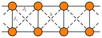
Figure 1: Orange circles mark spin sites, solid black lines mark Heisenberg interaction. Dashed diagonal lines indicate the pertubation.

We consider two types of initial states. The first initial state is given by

$$\rho_{1}(0)\propto 1-\varepsilon\,S^{z}_{L/2}\,,$$ (10)

where $\varepsilon$ is a small, positive, real number. This state can be regarded as the high temperature, strong magnetic field limit ($\beta\rightarrow 0$ while $\beta B=\varepsilon$) of the Gibbs state

$$\rho_{2}(0)\propto\text{exp}[-\beta(H+BS^{z}_{L/2})]\,,$$ (11)

which is the second initial state of interest.

IV Numerical Results on the perturbed dynamics

We now present our numerical results. We prepare a spin ladder with $L=13$ rungs (i.e. $N=26$ spins) in the initial states mentioned aboved, which both feature a sharp magnetization peak in the middle of the ladder. During the real time evolution the magnetization will spread throughout the ladder diffusively Richter et al. (2019b), which can be seen in Fig. 2.

From Eq. (8) we obtain the Fourier modes of the broadening process. We choose to investigate the slowest mode with $q=2\pi/13$ in depth since it is closest to an exponential decay. In Fig. 3 the slowest mode is depicted for different pertubation strengths for the first initial state $\rho_{1}(0)$. The unperturbed dynamic (red curve, $\lambda=0.0$) remains basically unaltered by weak pertubations. Cranking up the pertubation strength (to $\lambda=0.4$ or $\lambda=0.7$) leads to a noticable deviation and the equilibration process is much slower than in the weakly perturbed case.
The same qualitative behavior remains when going to finite temperature $\beta=0.1$ and finite magnetic field $B=5.0$.

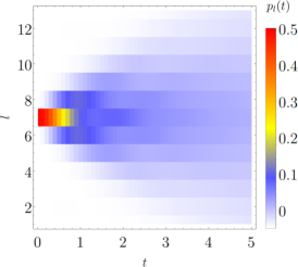
Figure 2: Broadening of the magnetization profile of a spin ladder with $L=13$ rungs prepared in the initial state $\rho_{1}(0)$ .

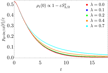
Figure 3: The time-dependence of the slowest mode with $q=2\pi/13$ is depicted for various pertubation strengths for the initial state $\rho_{1}(0)$. For small pertubations the unpertubed dynamic ($\lambda=0.0$, red curve) remains basically unchanged. For stronger pertubations there is a noticeable deviation.

In this case, the initial value $p_{q}(0)$ depends on the pertubation strength $\lambda$ since the total Hamiltonian is part of the initial state $\rho_{2}(0)$, cf. Eq. (11). To be able to compare the dynamics for various $\lambda$, the curves are scaled such that they all start at the same initial value of the unperturbed dynamic. The results are depicted in Fig. 4. For weak pertubations the deviation from the unperturbed dynamic is again small, although now clearly visible. For stronger pertubations the dynamics equilibrate again more slowly, however, the discrepancy to the unperturbed dynamic is more severe compared to the first initial state $\rho_{1}(0)$ in Fig. 3. A rough estimate indicates that at inverse temperature $\beta=0.1$ the mean energy is down-shifted by approximately half a standard deviation of the full energy spectrum of the system with respect to the infinite temperature case ($\beta=0$). Thus, $\beta=0.1$ is noticeable far away from infinite temperature while still not exhibiting low temperature phenomena.

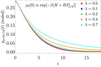
Figure 4: The time-dependence of the slowest mode with $q=2\pi/13$ is depicted for various perturbation strengths for a Gibbsian initial state $\rho_{2}(0)$ with $\beta=0.1$ and $B=5.0$. Similar behavior as for the first initial state can be observed.

V Modelling the perturbed dynamics

Is it possible to describe the observed behavior to some extend by any the three theories mentioned in the introduction? Before we present a somewhat bold, simple comparison of the predictions from said modeling schemes with the actual perturbed dynamics, we briefly comment on the agreement of our setup (cf. Sect. III) with the preconditions of the respective theories.

The theory advocated in Ref. Dabelow and Reimann (2020) relies on a constant density of states (DOS) within the energy interval occupied by the initial state $\rho(0)$ with respect to the unperturbed Hamiltonian $H_{0}$.First of all it should be noted that it is rather hard to check whether or not this criterion applies in standard situations with larger systems. However, a histogram corresponding to the DOS of $H_{0}$ for a “small” system with $N=12$ spins is depicted in Fig. 5. The red dashed vertical lines are intended to mark the regime of more or less constant DOS (of course this choice is rather arbitrary). The initial state $\rho_{1}(0)$ populates the full spectrum with equal weight, i.e. $57\%$ of the weight falls into the interval of approximately constant DOS. Likewise, although populating more low-lying energy eigenstates, a large portion ($54\%$) of the weight of the initial state $\rho_{2}(0)$ still falls into the interval of approximately constant DOS, cf. Fig. 5.

The assessment of this finding is twofold: On the one hand, “natural” initial states like $\rho_{1}(0)$ and $\rho_{2}(0)$ do not necessarily live entirely in an energy window of strictly constant DOS. On the other hand, Fig. 5 indicates that the states $\rho_{1}(0)$ and $\rho_{2}(0)$ are not completely off such a description. One may thus be inclined to expect at least qualitatively reasonable results from an application of the theory presented in Ref. Dabelow and Reimann (2020). Concerning perturbations $V$, the approach in Ref. Dabelow and Reimann (2020) strictly speaking makes no restrictions, except for “smallness”. But the result from Ref. [8] is of statistical nature: To the overwhelming majority of the ensemble of matrices $V$ that is generatated by drawing matrix elements in the eigenbasis of $H_{0}$ independently at random (according to some probability distribution, which may give rise to some sparseness) the prediction of Ref. Dabelow and Reimann (2020) (exponential damping) applies. While any $V$ may be viewed as an instance of this set, not all $V$ are equally likely. Again, judging the “typicality” of some concrete $V$ is hard. However, for a qualitative evaluation of the typicality of the pertubation $V$ at hand with respect to the above ensemble, a color-scaled plot of $V$ in the energy eigenbasis of $H_{0}$ for $N=12$ is depicted in Fig. 6. The red lines correspond to the energy regime marked in Fig. 5. Obviously, there is some sparseness, about $2\%$ of all elements differ from zero. Other than that the assessment of this finding is also twofold: On the one hand, some structure is visible in Fig. 6. On the other hand, this structure is not sufficient to clearly identify $V$ as particularly untypical. Hence, again, one may be inclined to expect at least qualitatively reasonable results from an application of the theory presented in Ref. [8].

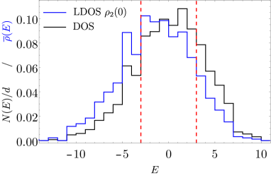
Figure 5: Density of states (black) for $N=12$ spins. The quantity $N(E)$ is the number of energy eigenstates in a particular bin of size one, $d=4096$ is the Hilbert space dimension. The interval of approximately constant DOS is marked from $E=-3\,\ldots\,3$ by red lines. A histogram of the local density of states (LDOS), i.e. the probability to find the system at a certain energy, is shown in blue. The quantity $\bar{\rho}(E)$ indicates the weight in a given bin. The LDOS of $\rho_{1}(0)$ is exactly identical to the DOS (black) and not shown again.

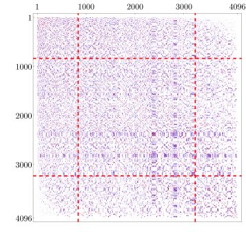
Figure 6: Matrix plot of the pertubation $V$ in the eigenbasis of the unperturbed Hamiltonian $H_{0}$. Red lines mark the interval of approximately constant DOS, cf. Fig. 5.

The theory advocated in Ref. Richter et al. (2019a) relies on projection operator techniques Breuer and Petruccione (2006) and thus has, in principle, no formal applicability limit. However, as projection operator techniques result in perturbative expansions, concrete predictions going beyond leading order are very hard to obtain Steinigeweg and Prosen (2013). Even the accurate computation of the leading order requires the knowledge of the detailed form of the matrix depicted in Fig. 6 has to be taken into account. The simple guess of an exponential damping at sufficiently long times only results under preconditions that are rather similar to the ones on which the approach from Ref. Dabelow and Reimann (2020) is based. The conditions under which the dynamics is well captured by a leading order description are technically hard to define and even harder to check. However, there are indications that the sparseness of the matrix depicted in Fig. 6 threatens the correctness of a leading order calculation Bartsch et al. (2008).

The approach advocated in Ref. Knipschild and Gemmer (2018) is heuristic and primarily based on some numerical evidence, thus no formal preconditions may be formulated so far, cf. Sect. II. However, the numerical examples in Ref. Knipschild and Gemmer (2018) to which this scheme applies do feature unperturbed Hamiltonians with constant DOS, weak perturbations (small $\lambda$) and initial states of the type $\rho_{1}(0)$. Furthermore the $V$’s in the examples in Ref. Knipschild and Gemmer (2018) are matrices whose elements, in the eigenbasis of the observable, are independently drawn at random according to some probability distribution. As already mentioned in Sect. II, in contrast to Refs. Dabelow and Reimann (2020); Richter et al. (2019a), the approach in Ref. Knipschild and Gemmer (2018) takes the structure of $V$ in the eigenbasis of the observable (here $S_{q}^{z}$) rather than of $H_{0}$ into account. Only if the latter approximately commute, i.e. $[V,A]\approx 0$, the prediction computed as described in Sect. II applies. For our setup we indeed have $[V,A]=0$, cf. Sect. III.

We now embark on the announced bold comparison of the perturbed dynamics with the predictions from the three theories.
Firstly, note that for both initial states the perturbed curves lie above the unperturbed one, i.e. the stronger the perturbation the slower the relaxation occurs. Thus, theories predicting a damping of the unperturbed dynamics are not a viable option in this case. Without any further quantitative analysis this already renders the predictions from Ref. Dabelow and Reimann (2020) and Ref. Richter et al. (2019a) qualitatively unsuitable. Moreover, it can be shown (at least for the first initial state) that all curves must feature zero slope at $t=0$. An exponential damping (with a constant damping factor) would always change the slope at $t=0$ to a non-zero value. A time-dependent damping factor $\Gamma(t)$ with $\Gamma(0)=0$ (as employed in Ref. Richter et al. (2019a)) at least preserves the zero slope at $t=0$.
These findings suggest that the pertubation $V$ is indeed one of the mathematically extremely untypical members of the ensemble considered in Ref. Dabelow and Reimann (2020), even though the matrix visualization in Fig. 6 does not necessarily indicate this. However, even though $V$ is untypical with respect to an ensemble of random matrices, it is a physically simple, common pertubation consisting of standard spin-spin interactions.

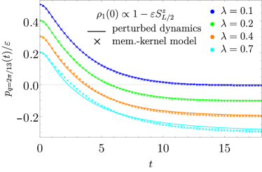
Figure 7: Slowest mode with $q=2\pi/13$ of the infinite-temperature initial state $\rho_{1}(0)$ depicted for various pertubation strengths. Solid lines represent the original data from Fig. 3, vertically shifted in steps of $-0.1$ for better visibility. Crosses indicate the data obtained from an exponentially damped memory-kernel.

The failure of the scheme presented in Ref. Richter et al. (2019a) indicates that the $V$ at hand does not allow for a leading order truncation of the projective scheme employed therein, not even for very small $\lambda$. This leaves the memory-kernel model from Ref. Knipschild and Gemmer (2018) as a the only feasible theory to describe the observed behavior.

In the following, to test the approach from Ref. Knipschild and Gemmer (2018), we apply the memory-kernel ansatz to the two unperturbed dynamics (red curves in Fig. 3 and Fig. 4). The damping constant $\gamma$ from Eq. (2) functions as a fit parameter and is optimized such that the $L^{2}$-error of the two curves in question (perturbed dynamics and memory-kernel prediction) is minimized.

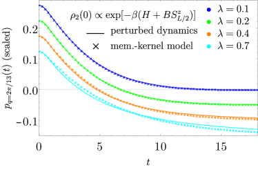
Figure 8: Slowest mode with $q=2\pi/13$ of the Gibbsian initial state $\rho_{2}(0)$ with $\beta=0.1$ and $B=5.0$ depicted for various pertubation strengths. Solid lines represent the original data from Fig. 4, vertically shifted in steps of $-0.05$ for better visibility. Crosses indicate the data obtained from an exponentially damped memory-kernel.

For the infinite-temperature initial state $\rho_{1}(0)$ the results are depicted in Fig. 7, for the Gibbsian initial state $\rho_{2}(0)$ the results are depicted in Fig. 8. Each curve is vertically shifted to avoid clutter. For the infinite-temperature initial state $\rho_{1}(0)$ and weak pertubations ($\lambda=0.1$ and $\lambda=0.2$) the memory-kernel model seems to perfectly capture the modified dynamics. For stronger pertubations ($\lambda=0.4$ and $\lambda=0.7$) there are deviations visible, e.g. for short times ($t\sim 2$) the memory-kernel prediction for $\lambda=0.7$ overshoots the perturbed dynamic while for longer times $t\gtrsim 10$ it undershoots. For the Gibbsian initial state $\rho_{2}(0)$ the qualitative behavior remains the same as for the first initial state. For weak pertubations the memory-kernel ansatz captures the modifications due to the pertubation extremly well. For stronger pertubations there are again more noticeable deviations. However, it comes as no surprise that the memory-kernel model looses potency in the strong pertubation regime, since it was originally conceived to describe the alteration of dynamics due to weak pertubations.

VI Summary and conclusion

In the paper at hand we numerically analyzed the applicability of three theories predicting the generic impact of Hamiltonian perturbations on expectation value dynamics to a Heisenberg spin ladder. To this end, we numerically calculated the time-dependent spatial distribution of the magnetization along the ladder for various pertubation strengths. We focused on a particular perturbation that commutes with the observable, e.g. the considered perturbation $V$ consisting of $S^{z}S^{z}$-couplings on the ladder diagonals commutes with the observed spatial magnetization distribution. We consider both, infinite and finite temperatures. Two out of three scrutinized theories feature in principle well defined conditions for their applicability Dabelow and Reimann (2020); Richter et al. (2019a), a third one is rather heuristic Knipschild and Gemmer (2018). One of the theories with well defined conditions Dabelow and Reimann (2020) only predicts the overwhelmingly likely behavior with respect to a hypothetical, large, “random matrix ensemble” of in principle possible perturbations $V$. Only the heuristic theory takes the the commutativity of the observable and the perturbation as a specifically relevant structural feature into account. It turns out to be hard to judge a priori whether or not the concrete spin ladder example falls into the realm of applicability of the two theories with well defiend condtions. However, direct comparison of the theoretical predictions with the numerically computed results clearly shows that both theories fail even qualitativley. This suggests that, while the the considered $V$ is very common from a physical point of view, it must be very rare and exotic with respect to the above random matrix ensemble. Only the heuristic theory was found to yield good results for weak perturbations (and acceptable results for strong perturbations). This indicates that the commutator of $V$ with the observable is a specifically relevant structural feature that should be taken into account. A survey of the three theories for perturbations $V$ that do not commute with the observable is left for further research.