Age-Aware Status Update Control for Energy Harvesting IoT Sensors via Reinforcement Learning

Abstract

We consider an IoT sensing network with multiple users, multiple energy harvesting sensors, and a wireless edge node acting as a gateway between the users and sensors. The users request for updates about the value of physical processes, each of which is measured by one sensor. The edge node has a cache storage that stores the most recently received measurements from each sensor. Upon receiving a request, the edge node can either command the corresponding sensor to send a status update, or use the data in the cache. We aim to find the best action of the edge node to minimize the average long-term cost which trade-offs between the age of information and energy consumption. We propose a practical reinforcement learning approach that finds an optimal policy without knowing the exact battery levels of the sensors. Simulation results show that the proposed method significantly reduces the average cost compared to several baseline methods.

I Introduction

Internet of Things (IoT) is a new technology which uses minimal human intervention and connects different devices and applications. IoT enables us to effectively interact with the physical surrounding environment and empower context-aware applications like smart cities [1]. A typical IoT sensing network consists of multiple wireless sensors which measure a physical quantity and communicate the measurements to a destination for further processing. Two special features of these networks are: 1) stringent energy limitations of battery-powered sensors which may be counteracted by harvesting energy from environmental sources like sun, heat, and RF ambient [2], and 2) transient nature of data, i.e., the sensors’ measurements become outdated after a while. Thus, it is crucial to design IoT sensing techniques where the sensors sample and send minimal number of measurements to prolong their lifetime while providing the end users highly fresh data for time-sensitive IoT applications. The freshness of information from the users’ perspective can be quantified by the recently emerged metric, the age of information (AoI) [3, 4, 5].

We consider an IoT sensing network consisting of multiple users, multiple energy harvesting IoT sensors, and a wireless edge node. The users send requests for the physical processes, each of which is measured by one sensor. The edge node, which acts as a gateway between the users and the sensors, has a cache storage which stores the most recently received measurements of each physical quantity. Upon receiving a request, the edge node can either command the corresponding sensor to sample and send a new measurement, or use the available data in the cache. The former leads to having a fresh measurement, yet at the cost of increased energy consumption. Since the latter prevents the activation of the sensors for every single request, the sensors can stay longer in a sleep mode to save a considerable amount of energy [6], but the data forwarded to the users becomes stale. This results in an inherent trade-off between the AoI of sensing data and sensors’ energy consumption.

Contributions: The main objective of this paper is to find the best action of the edge node at each time slot, which is called an optimal policy, to strike a balance between the AoI and energy consumption in the considered IoT sensing network. We address a realistic scenario where the edge node does not know the exact battery level of each energy harvesting sensor at each time slot, but only the level from a sensor’s last update. We model the problem of finding an optimal policy as a Markov decision process (MDP). We propose a reinforcement learning (RL) based algorithm to obtain an optimal policy that minimizes a cost function that trade-offs the AoI and energy consumption. Simulation results show that the proposed method significantly reduces the average cost compared to several baseline methods.

Related works: RL is an online machine learning method which learns an optimal policy through the interactions between the agent (the edge node in our case) and the environment. A comprehensive survey of RL based methods for autonomous IoT networks is presented in [7]. In [8, 9], the authors used RL to find an optimal caching policy for non-transient data (e.g., multimedia files). In [10], deep RL was used to minimize AoI in a real-time multi-node monitoring system, in which the sensors are powered through wireless energy transfer by the destination. The authors in [11] used deep RL to solve a cache replacement problem with a limited cache size and transient data in an IoT network. Different from [11], we consider both energy harvesting and energy limitation of the IoT sensors. The authors in [6] considered a known energy harvesting model and proposed a threshold adaptation algorithm to maximize the hit rate in an IoT sensing network. Compared to [6], we include data freshness/AoI and, by assuming that the energy harvesting model is unknown, use RL to search for the optimal policy.

II System Model and Problem Formulation

II-A Network Model

We consider an IoT sensing network consisting of multiple users (data consumers), a wireless edge node, and a set of $K$ energy harvesting sensors (data producers), as depicted in Fig. 1. Sensor $k\in\mathcal{K}=\left\{1,\dots,K\right\}$ measures independently a specific physical quantity $f_{k}$, e.g., temperature or humidity. The system operates in a slotted fashion, i.e., time is divided into slots which are labeled with a discrete index ${t\in\mathbb{N}}$.

We assume that there is no direct link between the users and the sensors, i.e., the edge node acts as a gateway between them. Users request for the values of physical quantities so that at each time slot, there can be multiple requests arriving at the edge node. We assume that the requests for the value of physical quantities come at the beginning of each slot and the edge node sends values to the users at the end of the same slot. Let $r_{k}(t)\in\{0,1\}$, $t=1,2,\dots$, denote the random process of requesting the value of $f_{k}$ at the beginning of slot $t$; $r_{k}(t)=1$ if the value of $f_{k}$ is requested and $r_{k}(t)=0$, otherwise.

The edge node is equipped with a cache storage that stores the most recently received measurement of each physical quantity. Upon receiving a request for the value of $f_{k}$ at slot $t$ (i.e., $r_{k}(t)=1$), the edge node can either command sensor $k$ to perform a new measurement and send a status update, or use the previous measurement in the local cache, to serve the request. Let $a_{k}(t)\in\{0,1\}$ denote the command action of the edge node at slot $t$; $a_{k}(t)=1$ if the edge node commands sensor $k$ to send a status update and $a_{k}(t)=0$ otherwise.

II-B Energy Harvesting Model

Sensors rely on the energy harvested from the environment. Sensor $k$ stores the harvested energy in a battery of finite size $B_{k}$ (units of energy). For defining the cost of transmitting a status update from each sensor to the edge node, we consider the common assumption (see e.g., [12, 13, 14, 15, 16]) that this transmission consumes one unit of energy. Let random variable $d_{k}(t)\in\left\{0,1\right\}$ denote the action of sensor $k$ at slot $t$; $d_{k}(t)=1$ if sensor $k$ sends a status update to the edge node and $d_{k}(t)=0$ otherwise. Note that $d_{k}(t)$ and $a_{k}(t)$ can be different which is discussed in Section II-C.

Let $b_{k}(t)$ denote the battery level of sensor $k$ at the beginning of slot $t$. The evolution of the battery level of sensor $k$ can be expressed as

$$b_{k}(t+1)=\min\left\{b_{k}(t)+e_{k}(t)-d_{k}(t),B_{k}\right\},$$ (1)

where $e_{k}(t)\in\left\{0,1\right\}$, $t=1,2,\dots$, is the energy arrival process of sensor $k$. We assume that the energy arrival processes are independent and unknown to the edge node. Moreover, the energy harvested during slot $t$ can be used only in a later slot.

II-C Status Update with Partial Knowledge of the Battery Levels

We consider a realistic environment in which the edge node is informed about the battery levels of the sensors only via the status update packets. Each status update packet consists of the value of $f_{k}$, the generation timestamp, and the battery level of sensor $k$. Let variable $\tilde{b}_{k}(t)$ denote the battery level of sensor $k$ at the beginning of that time slot in which the most recent status update of sensor $k$ was received by the edge node. Thus, the edge node does not know the exact battery level of the sensors at each time slot, but it only has the partial knowledge, i.e., the level from the sensor’s last update, $\tilde{b}_{k}(t)$.

Due to the partial knowledge of the battery levels at the edge node, it may happen that the edge node commands sensor $k$ to send a status update (i.e., $a_{k}(t)=1$), while sensor $k$ has run out of battery (i.e., $b_{k}(t)=0$). Consequently, the sensor can not send a status update (i.e., $d_{k}(t)=0$). In this case, the edge node does not receive any status update from the sensor during slot $t$, and thus, serves the user’s request using the previous measurement from the local cache.

In conclusion, sensor $k$ sends a status update packet only whenever it is commanded by the edge node and it has at least one unit of energy in its battery, i.e.,

$$d_{k}(t)=a_{k}(t)\mathds{1}_{\{b_{k}(t)>0\}},$$ (2)

where $\mathds{1}_{\{.\}}$ is the indicator function.

Figure 1: IoT sensing network consisting of multiple users (data consumers), one wireless edge node (i.e., the gateway), and a set of $K$ energy harvesting wireless IoT sensors (data producers). The procedure of serving a request by using fresh data is shown by green lines, and the blue lines show the procedure of serving a request by using the previous measurements already existing in the cache.

II-D Age of Information

Age of information (AoI) is a destination-centric metric that quantifies the freshness of information of a remotely observed random process [3, 4, 5]. Formally, AoI is the time elapsed since the generation of the last received status update packet. Let $\Delta_{k}(t)$ be the age of the value of $f_{k}$ at the edge node at the beginning of slot $t$, i.e., the number of slots elapsed since the generation timestamp of the last received status update packet from sensor $k$. More precisely, $\Delta_{k}(t)=t-u_{k}(t)$ where $u_{k}(t)$ represents the most recent time slot in which the edge node received a status update packet from sensor $k$, i.e., $u_{k}(t)=\max\{t^{\prime}|t^{\prime}<t,d_{k}(t^{\prime})=1\}$. Accordingly, the evolution of $\Delta_{k}(t)$ can be written as

$$\Delta_{k}(t+1)=\begin{cases}\Delta_{k}(t)+1,&\text{if}\leavevmode\nobreak\ d_{k}(t)=0\\ 1,&\text{if}\leavevmode\nobreak\ d_{k}(t)=1,\end{cases}$$ (3)

which can be expressed compactly as $\Delta_{k}(t+1)=\left(1-d_{k}(t)\right)\Delta_{k}(t)+1$.

II-E Cost Function and Problem Formulation

We consider a cost function that has two components: one penalizes the energy consumption (characterized by $d_{k}(t)$) and the other one penalizes the information staleness. More precisely, we define the cost of serving a request for the value of physical quantity $f_{k}$ at slot $t$ (i.e., $r_{k}(t)=1$) as

$$c_{k}(t)=(1-\beta)d_{k}(t)+\beta r_{k}(t)g_{k}(\Delta_{k}(t+1)),$$ (4)

where a weighting parameter $\beta\in[0,1]$ determines the trade-off between the emphasis on energy consumption and information staleness, and $g_{k}(\cdot)$ is an increasing function of AoI (see e.g. [17, 18, 19]).

We aim to find the best action of the edge node at each time slot, which is called an optimal policy, that minimizes the time-average accumulated cost, defined as

$$\bar{C}=\displaystyle\underset{T\rightarrow\infty}{\mathrm{lim}}\frac{1}{T}\displaystyle\sum_{t=1}^{T}\displaystyle\sum_{k=1}^{K}c_{k}(t).$$ (5)

The cost in (5) can be equivalently expressed as

$${\bar{C}=\sum_{k=1}^{K}\bar{C}_{k}},$$ (6)

where $\bar{C}_{k}$ is the time-average accumulated cost associated with sensor $k$, defined as

$$\bar{C}_{k}=\displaystyle\underset{T\rightarrow\infty}{\mathrm{lim}}\frac{1}{T}\displaystyle\sum_{t=1}^{T}c_{k}(t),\leavevmode\nobreak\ k=1,\dots,K.$$ (7)

Remark 1.

Focusing on finding $a_{k}(t)$, $k\in\mathcal{K}$, that minimizes (5), we conclude that the above problem is separable across $k$. Namely, the decisions of the edge node for each sensor do not affect the decisions for the others, i.e., the actions $a_{k}(t)$ are independent across $k\in\mathcal{K}$.

By Remark 1, minimizing the system-wise cost in (5) reduces to minimizing the $K$ per-sensor time-average accumulated costs in (7). This will be a key factor for developing our algorithm in Section III.

Remark 2.

Note that in searching for the policy that minimizes (7), only the selection of those actions $a_{k}(t)$ for which $r_{k}(t)=1$ needs to be optimized. Namely, it is clear that if $r_{k}(t)=0$, the best action is $a_{k}(t)=0$; this implies $d_{k}(t)=0$, and consequently, $c_{k}(t)=0$.

In the next section, we model the problem of minimizing the average cost over all sensors in (5) (which is equal to minimizing $K$ per-sensor average costs in (7)) as a Markov decision process (MDP) and search for the optimal policy using reinforcement learning (RL) [20].

III Reinforcement Learning Based Status Update Policy

In this section, we model the problem of finding an optimal policy at the edge node as an MDP and propose a Q-learning based algorithm to find an optimal policy that minimizes the expected long-term cost. As a key advantage, the proposed algorithm is simple with low complexity of implementation, which is an important point in practice.

III-A MDP Modeling

The MDP model can be defined by the tuple ${\left\{\mathcal{S},\mathcal{A},\mathcal{P}\left(s(t+1)|s(t),a(t)\right),c(t),\gamma\right\}}$, where

• $\mathcal{S}=\mathcal{S}_{1}\times\dots\times\mathcal{S}_{K}$ is the set of system states, where $\mathcal{S}_{k}$ is the per-sensor state set. Let $s(t)\in\mathcal{S}$ denote the state at slot $t$, which is equal to $s(t)=\left\{s_{1}(t),\dots,s_{K}(t)\right\}$. At each time slot, the per-sensor state $s_{k}(t)\in\mathcal{S}_{k}$ is characterized by 1) partial knowledge about the battery level of sensor $k$, i.e., $\tilde{b}_{k}(t)=b_{k}(u_{k}(t))$, and 2) the AoI of the value of $f_{k}$ in the local cache $\Delta_{k}(t)$. Thus, $s_{k}(t)=\left\{\tilde{b}_{k}(t),\Delta_{k}(t)\right\}$. It is important to point out that the state contains $\tilde{b}_{k}(t)$ instead of $b_{k}(t)$, because the edge node is unaware of the exact battery level of sensor $k$ at slot $t$.

• $\mathcal{A}=\mathcal{A}_{1}\times\dots\times\mathcal{A}_{K}$ is the action set, where $\mathcal{A}_{k}=\left\{0,1\right\}$ is the per-sensor action set. The action selected by the edge node at slot $t$ is denoted by $a(t)\in\mathcal{A}$, which is defined as $a(t)=\left\{a_{1}(t),\dots,a_{K}(t)\right\}$, $a_{k}(t)\in\mathcal{A}_{k}$.

• $\mathcal{P}\left(s(t+1)|s(t),a(t)\right)$ is the state transition probability that maps a state-action pair at time slot $t$ onto a distribution of states at time slot $t+1$.

• $c(t)$ is the immediate cost function, i.e., the cost of taking action $a(t)$ in state $s(t)$, which is defined as $c(t)=\left\{c_{1}(t),\dots,c_{K}(t)\right\}$.

• $\gamma\in\left(0,1\right]$ is the discount factor used to weight the immediate cost relative to the future costs. In general, the factor $\gamma$ is smaller than one to guarantee that the cumulative reward is finite, given that the immediate cost is bounded [20].

The long-term accumulated cost is defined as

$$C(t)=\displaystyle\sum_{k=1}^{K}C_{k}(t),$$ (8)

where ${C_{k}(t)=\textstyle\sum_{\tau=0}^{\infty}\gamma^{\tau}c_{k}(\tau+t)}$. Formally, policy $\pi=\pi(a(t)|s(t))$ is defined as a mapping from state $s(t)$ to a probability of choosing action $a(t)$. Note that $\pi=\left\{\pi_{1},\dots,\pi_{K}\right\}$, where $\pi_{k}=\pi_{k}(a_{k}(t)|s_{k}(t))$, $k\in\mathcal{K}$. Our optimization problem is to find an optimal policy that minimizes the expected long-term accumulated cost over all sensors, i.e., $\pi^{*}=\operatorname*{arg\,min}_{\pi}\mathbb{E_{\pi}}\left[C(t)\mid\pi\right]$. According to Remark 1, the optimization problem is separable across $k$, and thus, $\pi^{*}=\left\{\pi^{*}_{1},\dots,\pi^{*}_{K}\right\}$ can be found by solving $K$ sub-problems

$$\pi^{*}_{k}=\operatorname*{arg\,min}_{\pi_{k}}\mathbb{E}_{\pi_{k}}\left[C_{k}(t)\mid\pi_{k}\right],\leavevmode\nobreak\ k\in\mathcal{K}.$$ (9)

The state-value and action-value functions are defined to evaluate a policy $\pi$. The state-value function of a state $s$ under a policy $\pi$, denoted by $v_{\pi}\left(s\right)$, is the expected return when starting in state $s$ and following the policy $\pi$ thereafter, i.e., $v_{\pi}\left(s\right)\doteq\mathbb{E}_{\pi}\left[C(t)|s(t)=s\right],\forall s\in\mathcal{S}$. The action-value function, denoted by ${q_{\pi}\left(s,a\right)}$, is the expected return for taking an action $a$ in state $s$ and thereafter following the policy $\pi$, i.e., $q_{\pi}\left(s,a\right)\doteq\mathbb{E}_{\pi}\left[C(t)|s(t)=s,a(t)=a\right],\forall s\in\mathcal{S},a\in\mathcal{A}$.

The optimal action-value function for state $s$ and action $a$ is defined as ${q^{*}\left(s,a\right)\doteq\min_{\pi}q_{\pi}\left(s,a\right)}$. If $q^{*}\left(s,a\right)$ is available, the optimal policy $\pi^{*}$ is obtained simply by choosing the action $a$ that minimizes $q^{*}\left(s,a\right)$ in each state. By using Remark 1, we have $q^{*}\left(s,a\right)=\sum_{k=1}^{K}q^{*}_{k}(s_{k}(t),a_{k}(t))$, where ${q^{*}_{k}\left(s,a\right)=\min_{\pi_{k}}q_{\pi_{k}}\left(s,a\right)}$ and $q_{\pi_{k}}\left(s,a\right)=\mathbb{E}_{\pi_{k}}\left[C_{k}(t)|s_{k}(t)=s,a_{k}(t)=a\right]$.

If the state transition probabilities $\mathcal{P}\left(s(t+1)|s(t),a(t)\right)$, $s\in\mathcal{S}$, $a\in\mathcal{A}$, are available, the optimal policy can be found by dynamic programming, e.g., by the model-based methods such as the value iteration algorithm [20, Ch.  4]. Since $\mathcal{P}\left(s(t+1)|s(t),a(t)\right)$ is unknown in our considered scenario, we use model-free RL to learn the action-value functions by experience.

III-B Online Q-learning Algorithm

Q-learning is an online model-free RL algorithm that finds the optimal policy iteratively. In the Q-learning method, the learned action-value function for sensor $k$, denoted as $Q_{k}$, $k\in\mathcal{K}$, directly approximates the optimal action-value function $q^{*}_{k}(s,a)$, $\forall s\in\mathcal{S}_{k},a\in\mathcal{A}_{k}$ [20, Sect. 6.5]. The convergence $Q_{k}\rightarrow q^{*}_{k}$ requires that all state-action pairs continue to be updated. To satisfy this condition, a typical approach is to use the ”exploration-exploitation” technique in the action selection. The $\epsilon$-greedy algorithm is one such method that trade-offs exploration and exploitation [20, Sect. 6.5].

Our proposed Q-learning algorithm is presented in Algorithm 1. To allow exploration-exploitation, the edge node takes either a random or greedy action at slot $t$; the probability of taking a random action is denoted by $\epsilon(t)$, and thus, the probability of exploiting the greedy action $a_{k}(t)=\operatorname*{arg\,min}_{a\in\mathcal{A}_{k}}Q_{k}(s_{k}(t),a)$ is $1-\epsilon(t)$. Generally, during initial iterations, it is better to set $\epsilon(t)$ high in order to learn the underlying dynamics, i.e., to allow more exploration. On the other hand, in stationary settings and once enough observations are made, small values of $\epsilon(t)$ become preferable to increase tendency to exploitation.

Algorithm 1 Status update control algorithm via Q-learning

1:  Initialize $Q_{k}(s,a)=0$, $\forall s\in\mathcal{S}_{k},a\in\mathcal{A}_{k}$, $k\in\mathcal{K}$

2:  for each slot $t=1,2,3,\dots$ do

3:     for $k=1,\dots,K$ do

4:        if $r_{k}(t)=0$ then

5:           $a_{k}(t)=0$

6:        else

7:           $a_{k}(t)$ is chosen according to the following probability$a_{k}(t)=\left\{\begin{array}[]{ll}\operatorname*{arg\,min}_{a\in\mathcal{A}_{k}}Q(s_{k}(t),a),\text{w.p.}1-\epsilon(t)\\ \textrm{a random action }a\in\mathcal{A}_{k},\text{w.p.}\hskip 14.22636pt\epsilon(t)\end{array}\right.$

8:           if $a_{k}(t)=1$ then

9:              Command sensor $k$ to send a status update packet

10:              if $b_{k}(t)>0$ then

11:                 $d_{k}(t)=1$

12:              else

13:                 $d_{k}(t)=0$

14:              end if

15:           else

16:              $d_{k}(t)=0$

17:           end if

18:        end if

19:        Update AoI according to (3) and calculate $c_{k}(t)$

20:     end for

21:     Wait for the next requests and compute $s(t+1)$

22:     for each sensor $k=1,\dots,K$ do {Update Q-tables}

23:        $\begin{array}[]{ll}Q_{k}\left(s_{k}(t),a_{k}(t)\right)\leftarrow(1-\alpha(t))Q_{k}\left(s_{k}(t),a_{k}(t)\right)\\ \hskip 22.76219pt+\alpha(t)\left(c_{k}(t)+\gamma\min_{a\in\mathcal{A}_{k}}Q_{k}\left(s_{k}(t+1),a\right)\right)\end{array}$

24:     end for

25:  end for

IV Simulation Results

In this section, simulation results are presented to demonstrate the benefits of the proposed Q-learning method summarized in Algorithm 1.

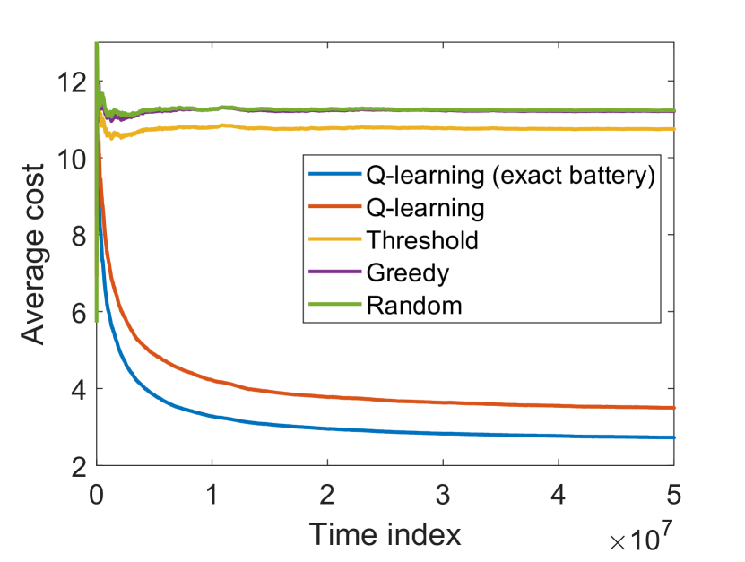
Figure 2: Convergence behavior of the proposed algorithm and baseline methods for weighting parameter $\beta=0.6$.

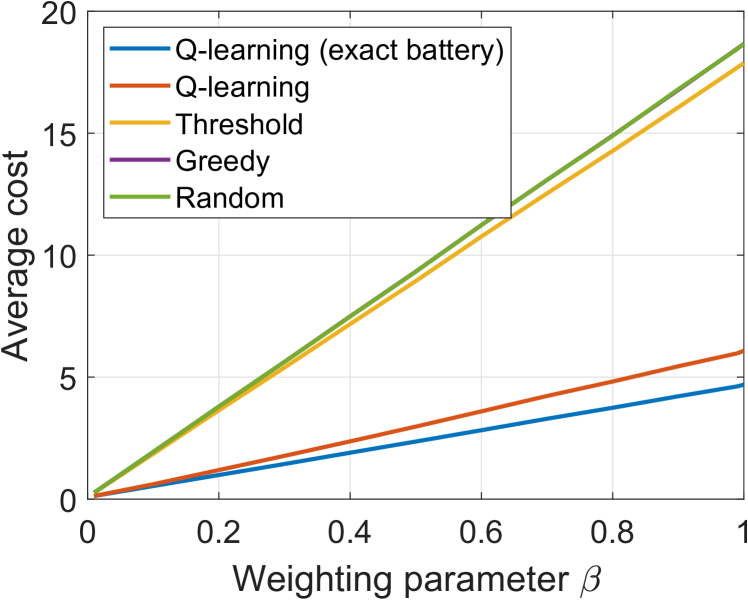
(a)

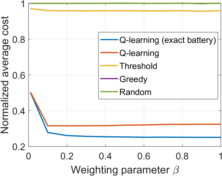
(b)

Figure 3: Performance of our Q-learning algorithm and other baseline methods as a function of weighting parameter $\beta$ in terms of (a) average cost and (b) normalized average cost.

IV-A Simulation Setup

The simulation scenario consists of $K=3$ energy harvesting sensors, i.e., $\mathcal{K}=\left\{1,2,3\right\}$. Each sensor has a battery of finite capacity $B=10$ units of energy. At each time slot the probability that the value of $f_{k}$ is requested (i.e., $r_{k}(t)=1$) is denoted by $p_{k}$, i.e., $\mathrm{Pr}\{r_{k}(t)=1\}=p_{k}$. We set $p_{k}=0.1$.

We model the underlying energy harvesting process of sensor $k$ as a two-state Markov chain with state space $\left\{V_{k,1},V_{k,2}\right\}$. For example, the states can represent ”good” and ”bad” energy harvesting states [16]. Let $V_{k}(t)$ denote the state of the environment at slot $t$ for sensor $k$. At slot $t$, if $V_{k}(t)=V_{k,1}$, sensor $k$ harvests one unit of energy (i.e., $e_{k}(t)=1$) with probability $\lambda_{k,1}$, i.e., $\mathrm{Pr}(e_{k}(t)=1|V_{k}(t)=V_{k,1})=\lambda_{k,1}$. Similarly, if $V_{k}(t)=V_{k,2}$, sensor $k$ harvests one unit of energy with probability $\lambda_{k,2}$. We denote the transition probability from state $V_{k,i}$ to state $V_{k,j}$ by $p_{k,ij}=\mathrm{Pr}(V_{k}(t)=V_{k,i}|V_{k}(t-1)=V_{k,j})$, $i,j\in\{1,2\}$. We set $\lambda_{k,1}=0.04$, $\lambda_{k,2}=0.0004$, $p_{k,11}=0.7$, $p_{k,12}=0.3$, $p_{k,21}=0.6$, and $p_{k,22}=0.4$, $k\in\mathcal{K}$.

For determining the cost function in (4), we define the function $g_{k}(\Delta_{k}(t+1))$ as

$$g_{k}(\Delta_{k}(t+1))={\left(\frac{\Delta_{k}(t+1)}{\zeta_{k}}\right)}^{\mu},$$ (10)

where ${\zeta_{k}}$ is the tolerance of using aged measurements of $f_{k}$, and ${\mu\geq 1}$ is a parameter that adjusts how aggressively we penalize when the AoI has a higher value than the tolerance of $f_{k}$, i.e., when ${\Delta_{k}(t+1)>\zeta_{k}}$. The function in (10) is a scaled version of a non-linear AoI; different functions for non-linear AoI have been investigated in [17, 18, 19]. Note that with $\mu=1$ and $\zeta_{k}=1$, $\forall{k}\in\mathcal{K}$, (10) is purely characterized by the AoI, i.e., $g(\Delta_{k}(t+1))=\Delta_{k}(t+1)$. We set $\mu=2$ and select $\zeta_{k}$ uniformly random from the interval $[3\ 15]$. Note that other functions are also applicable, e.g., $g(\Delta_{k}(t+1))=\textrm{log}(1+\Delta_{k}(t+1))$ [17].

In Algorithm 1, we set $\epsilon(t)=0.02+0.98e^{-\epsilon_{\textrm{d}}t}$ with decay parameter $\epsilon_{\textrm{d}}=0.01$, and the discount factor as $\gamma=0.99$. The learning rate $\alpha(t)$ is set to $\alpha(t)=0.5$ during the first $1/\epsilon_{\textrm{d}}=100$ iterations and after that $\alpha(t)=0.1$.

We evaluate the performance of the proposed algorithm in terms of average cost defined in (5). Three baseline policies are considered: greedy, threshold, and random. In the greedy policy, whenever the value of $f_{k}$ is requested (i.e., $r_{k}(t)=1$), the edge node commands sensor $k$ to send a status update (i.e., $a_{k}(t)=1$); sensor $k$ sends a status update if the battery is non-empty, $b_{k}(t)>0$. In the threshold policy, whenever the value of $f_{k}$ is requested (i.e., $r_{k}(t)=1$) and $\Delta_{k}(t)+1>\zeta_{k}$, the edge node commands sensor $k$ to send a status update. In the random policy, a random action $a_{k}(t)\in\{0,1\}$ is selected at each time slot. For the benchmarking, we also consider a genie-aided Q-learning method that knows the exact battery level of all sensors at each time slot. This policy serves clearly as a lower bound to the proposed Q-learning algorithm.

IV-B Results

Fig. 2 depicts the learning curves of each algorithm for weighting parameter ${\beta=0.6}$. The proposed Q-learning algorithm significantly outperforms other baseline methods; the decrease of the average cost is roughly threefold compared to the threshold algorithm, which has the best performance among the baseline policies here. Interestingly, the gap between the proposed Q-learning algorithm and the genie-aided Q-learning algorithm is small. This demonstrates that the proposed algorithm has high performance even it only has the partial knowledge about the battery levels of the sensors at each time slot, which is the case in practice.

Next, we focus on the average cost obtained by averaging each algorithm over $5$ episodes where each episode takes $3\times 10^{7}$ iterations. Fig. 3(a) illustrates the average cost of each algorithm for different values of weighting parameter $\beta$. For better visualization, Fig. 3(b) depicts a normalized average cost of each algorithm, defined as the ratio of the average cost of each algorithm to the average cost of the random policy. As shown in Fig. 3(a), when $\beta$ increases, the average cost increases for all algorithms, because the second term of (4) is squared ($\mu=2$) (see (10)). As shown in Fig. 3(b), for all values of $\beta$, the proposed Q-learning algorithm, which does not know the exact battery levels, performs close to the genie-aided Q-learning algorithm. Furthermore, the Q-learning algorithm reduces the average cost approximately by a factor of 3 compared to the threshold algorithm.

V Conclusions

We investigated a status update control problem in an IoT sensing network consisting of multiple users, multiple energy harvesting sensors, and a wireless edge node. We modeled the problem as an MDP and proposed an RL based algorithm that finds an optimal status update control policy that minimizes the average long-term cost which strikes a balance between the AoI and energy consumption. The proposed scheme does not need any information about the energy harvesting model and the exact battery level of the sensors. Simulation results showed the advantage of the proposed Q-learning algorithm.

VI Acknowledgments

This research has been financially supported by the Infotech Oulu, the Academy of Finland (grant 323698), and Academy of Finland 6Genesis Flagship (grant 318927). The work of M. Leinonen has also been financially supported in part by the Academy of Finland (grant 319485). M. Codreanu would like to acknowledge the support of the European Union’s Horizon 2020 research and innovation programme under the Marie Skłodowska-Curie Grant Agreement No. 793402 (COMPRESS NETS).

References

- [1] L. D. Xu, W. He, and S. Li, “Internet of things in industries: A survey,” IEEE Trans. Ind. Informat., vol. 10, no. 4, pp. 2233–2243, Nov. 2014.
- [2] S. Kim, R. Vyas, J. Bito, K. Niotaki, A. Collado, A. Georgiadis, and M. M. Tentzeris, “Ambient RF energy-harvesting technologies for self-sustainable standalone wireless sensor platforms,” Proc. IEEE, vol. 102, no. 11, pp. 1649–1666, Nov. 2014.
- [3] S. Kaul, R. Yates, and M. Gruteser, “Real-time status: How often should one update?” in Proc. IEEE Int. Conf. on Computer. Commun. (INFOCOM), Orlando, FL, USA, Mar. 25–30, 2012, pp. 2731–2735.
- [4] R. D. Yates and S. K. Kaul, “The age of information: Real-time status updating by multiple sources,” IEEE Trans. Inf. Theory, vol. 65, no. 3, pp. 1807–1827, Mar. 2019.
- [5] M. Costa, M. Codreanu, and A. Ephremides, “On the age of information in status update systems with packet management,” IEEE Trans. Inf. Theory, vol. 62, no. 4, pp. 1897–1910, Apr. 2016.
- [6] D. Niyato, D. I. Kim, P. Wang, and L. Song, “A novel caching mechanism for internet of things (IoT) sensing service with energy harvesting,” in Proc. IEEE Int. Conf. Commun., Kuala Lumpur, Malaysia, May 22-27 2016, pp. 1–6.
- [7] L. Lei, Y. Tan, S. Liu, K. Zheng, and X. Shen, “Deep reinforcement learning for autonomous internet of things: Model, applications and challenges,” arXiv preprint arXiv:1907.09059, 2019.
- [8] M. Hatami, M. Leinonen, and M. Codreanu, “Online caching policy with user preferences and time-dependent requests: A reinforcement learning approach,” in Proc. Annual Asilomar Conf. Signals, Syst., Comp., Pacific Grove, CA, USA, Nov. 3–6, 2019, pp. 1384–1388.
- [9] A. Sadeghi, F. Sheikholeslami, and G. B. Giannakis, “Optimal and scalable caching for 5G using reinforcement learning of space-time popularities,” IEEE J. Sel. Topics Signal Process., vol. 12, no. 1, pp. 180–190, Feb. 2018.
- [10] M. A. Abd-Elmagid, N. Pappas, and H. S. Dhillon, “A reinforcement learning framework for optimizing age-of-information in RF-powered communication systems,” arXiv preprint arXiv:1908.06367, 2019.
- [11] H. Zhu, Y. Cao, X. Wei, W. Wang, T. Jiang, and S. Jin, “Caching transient data for internet of things: A deep reinforcement learning approach,” IEEE Internet Things J., vol. 6, no. 2, pp. 2074–2083, Apr. 2019.
- [12] B. T. Bacinoglu, E. T. Ceran, and E. Uysal-Biyikoglu, “Age of information under energy replenishment constraints,” in Proc. Inform. Theory and Appl. Workshop, San Diego, CA, USA, Feb. 1–6 2015, pp. 25–31.
- [13] A. Arafa and S. Ulukus, “Timely updates in energy harvesting two-hop networks: Offline and online policies,” IEEE Trans. Wireless Commun., vol. 18, no. 8, pp. 4017–4030, Aug. 2019.
- [14] X. Wu, J. Yang, and J. Wu, “Optimal status update for age of information minimization with an energy harvesting source,” IEEE Trans. Green Commun. Netw., vol. 2, no. 1, pp. 193–204, Mar. 2018.
- [15] A. Arafa, J. Yang, S. Ulukus, and H. V. Poor, “Age-minimal transmission for energy harvesting sensors with finite batteries: Online policies,” IEEE Trans. Inf. Theory, vol. 66, no. 1, pp. 534–556, Jan. 2020.
- [16] N. Michelusi, K. Stamatiou, and M. Zorzi, “Transmission policies for energy harvesting sensors with time-correlated energy supply,” IEEE Trans. Commun., vol. 61, no. 7, pp. 2988–3001, Jul. 2013.
- [17] A. Kosta, N. Pappas, A. Ephremides, and V. Angelakis, “Age and value of information: Non-linear age case,” in Proc. IEEE Int. Symp. Inform. Theory, Aachen, Germany, Jun. 25–30 2017, pp. 326–330.
- [18] X. Zheng, S. Zhou, Z. Jiang, and Z. Niu, “Closed-form analysis of non-linear age of information in status updates with an energy harvesting transmitter,” IEEE Trans. Wireless Commun., vol. 18, no. 8, pp. 4129–4142, Jun. 2019.
- [19] Y. Sun and B. Cyr, “Sampling for data freshness optimization: Non-linear age functions,” IEEE J. Commun. Netw., vol. 21, no. 3, pp. 204–219, Jun. 2019.
- [20] R. S. Sutton and A. G. Barto, Reinforcement Learning: An Introduction, 2nd ed. Cambridge, MA, USA: MIT Press, 2018.