Approximate Turing Kernelization for Problems Parameterized by Treewidth

Abstract

We extend the notion of lossy kernelization, introduced by Lokshtanov et al. [STOC 2017], to approximate Turing kernelization. An $\alpha$-approximate Turing kernel for a parameterized optimization problem is a polynomial-time algorithm that, when given access to an oracle that outputs $c$-approximate solutions in $\mathcal{O}(1)$ time, obtains an $\alpha\cdot c$-approximate solution to the considered problem, using calls to the oracle of size at most $f(k)$ for some function $f$ that only depends on the parameter.

Using this definition, we show that Independent Set parameterized by treewidth $\ell$ has a $(1+\varepsilon)$-approximate Turing kernel with $\mathcal{O}(\frac{\ell^{2}}{\varepsilon})$ vertices, answering an open question posed by Lokshtanov et al. [STOC 2017]. Furthermore, we give $(1+\varepsilon)$-approximate Turing kernels for the following graph problems parameterized by treewidth: Vertex Cover, Edge Clique Cover, Edge-Disjoint Triangle Packing and Connected Vertex Cover.

We generalize the result for Independent Set and Vertex Cover, by showing that all graph problems that we will call friendly admit $(1+\varepsilon)$-approximate Turing kernels of polynomial size when parameterized by treewidth. We use this to obtain approximate Turing kernels for Vertex-Disjoint $H$-packing for connected graphs $H$, Clique Cover, Feedback Vertex Set and Edge Dominating Set.

1 Introduction

Many important computational problems are $\mathsf{NP}$-hard and, thus, they do not have efficient algorithms unless $\mathsf{P}=\mathsf{NP}$. At the same time, it is well known that efficient preprocessing can greatly speed up (exponential-time) algorithms for solving $\mathsf{NP}$-hard problems. The notion of a kernelization from parameterized complexity has allowed a rigorous and systematic study of this important paradigm. The central idea is to relate the effectiveness of preprocessing to the structure of the input instances, as quantified by suitable parameters.

A parameterized problem consists of any (classical) problem together with a choice of one or more parameters; we use $(x,k)$ to denote an instance with input data $x$ and parameter $k$. A kernelization is an efficient algorithm that on input of $(x,k)$ returns an equivalent instance $(x^{\prime},k^{\prime})$ of size upper bounded by $f(k)$, where $f$ is a computable function. For a polynomial kernelization we require that the size bound $f(k)$ is polynomially bounded in $k$. The study of which parameterized problems admit (polynomial) kernelizations has turned into a very active research area within parameterized complexity (see, e.g., [DBLP:conf/soda/AgrawalM0Z19, BodlaenderFLPST16_metakernelization, DBLP:conf/esa/00010SY18, DBLP:conf/wads/ChaplickFGK019, DBLP:conf/focs/FominLMS12, DBLP:conf/stacs/HolsK19, DBLP:conf/esa/JansenP18, DBLP:conf/stacs/JansenPL19, DBLP:conf/focs/KratschW12, DBLP:conf/stacs/2019, DBLP:conf/sofsem/WitteveenBT19] and the recent book [fomin_lokshtanov_saurabh_zehavi_2019]). An important catalyst for this development lies in the ability to prove lower bounds for kernelizations, e.g., to conditionally rule out polynomial kernels for a problem, which was initiated through work of Bodlaender et al. [BodlaenderDFH09] and Fortnow and Santhanam [FortnowS11].

Unfortunately, the lower bound tools have also revealed that many fundamental parameterized problems do not admit polynomial kernelizations (unless $\mathsf{NP\subseteq coNP/poly}$ and the polynomial hierarchy collapses). These include a variety of problems like Connected Vertex Cover [DomLS14], Disjoint Cycle Packing [DBLP:journals/tcs/BodlaenderTY11], Multicut [CyganKPPW14], and $k$-Path [BodlaenderDFH09] parameterized by solution size, but also essentially any $\mathsf{NP}$-hard problem parameterized by width parameters such as treewidth. This has motivated the study of relaxed forms of kernelization, notably Turing kernelization [Binkele-RaibleFFLSV12] and lossy (or approximate) kernelization [DBLP:conf/stoc/LokshtanovPRS17].

Given an input $(x,k)$, a Turing kernelization may create $|x|^{\mathcal{O}(1)}$ many instances of size at most $f(k)$ each, and the answer for $(x,k)$ may depend on solutions for all those instances. This is best formalized as an efficient algorithm that solves $(x,k)$ while being allowed to ask questions of size at most $f(k)$ to an oracle. A priori, this is much more powerful than regular kernelization, which creates only a single output instance. Nevertheless, there are only few polynomial Turing kernelizations known for problems without (regular) polynomial kernelization (e.g., [Binkele-RaibleFFLSV12, DBLP:conf/soda/JansenM15, DBLP:journals/jcss/Jansen17, DBLP:journals/algorithmica/ThomasseTV17]). Moreover, a hardness-based approach of Hermelin et al. [HermelinKSWW15] gives evidence that many problems are unlikely to admit polynomial Turing kernels.

More recently, Lokshtanov et al. [DBLP:conf/stoc/LokshtanovPRS17] proposed a framework dedicated to the study of lossy kernelization. This relaxes the task of the kernelization by no longer requiring that an optimal solution to the output $(x^{\prime},k^{\prime})$ yields an optimal solution for $(x,k)$. Instead, for an $\alpha$-approximate kernelization any $c$-approximate solution to $(x^{\prime},k^{\prime})$ can be lifted to an $\alpha\cdot c$-approximate solution for $(x,k)$. Amongst others, they show that Connected Vertex Cover and Disjoint Cycle Packing admit approximate kernelizations. In contrast, they were able to show, e.g., that $k$-Path has no $\alpha$-approximate kernelization for any $\alpha\geq 1$ (unless $\mathsf{NP\subseteq coNP/poly}$). Subsequent works have shown approximate kernelizations for other problems [DBLP:conf/mfcs/EibenHR17, DBLP:journals/siamdm/EibenKMPS19, DBLP:conf/esa/Ramanujan19], in particular, further problems with connectivity constraints, which are often an obstruction for the existence of polynomial kernelizations.

Lokshtanov et al. [DBLP:conf/stoc/LokshtanovPRS17] ask whether Independent Set parameterized by treewidth admits a polynomial-size approximate Turing kernelization with constant approximation ratio. In the present work, we answer this question affirmatively and in fact provide an efficient polynomial size approximate Turing kernelization scheme (EPSATKS). Moreover, extending the ideas for Independent Set, we provide similar results for a variety of other problems.

Our results

We prove that there is an EPSATKS for a wide variety of graph problems when parameterized by treewidth. The simplest problems we consider are the Vertex Cover and Independent Set problem. Observe that both problems parameterized by treewidth can be shown to be $\mathsf{MK}[2]$-hard, by a simple reduction from CNF-Sat with unbounded clause size. As such, for both problems we indeed do not expect polynomial Turing kernels [HermelinKSWW15]. We show that Vertex Cover has a $(1+\varepsilon)$-approximate Turing kernel with $\mathcal{O}(\frac{\ell}{\varepsilon})$ vertices, and Independent Set has a kernel with $\mathcal{O}(\frac{\ell^{2}}{\varepsilon})$ vertices.

Both approximate Turing kernels follow a similar strategy, based on using separators (originating from the tree decomposition) that separate a piece from the rest of the graph, such that the solution size in this piece is appropriately bounded. For this reason, we formulate a set of conditions on a graph problem and we call graph problems that satisfy these conditions friendly. We then show that all friendly graph optimization problems have polynomial-size $(1+\varepsilon)$-approximate Turing kernels for all $\varepsilon>0$, when parameterized by treewidth. Precise bounds on the size of the obtained approximate Turing kernels depend on properties of the considered problem, such as the smallest-known (approximate) kernel when parameterized by solution size plus treewidth. In particular, applying the general result for Vertex Cover indeed shows that it has an EPSATKS of size $\mathcal{O}(\frac{\ell}{\varepsilon})$. Using this general technique, we obtain approximate Turing kernels for Clique Cover, Vertex-Disjoint $H$-Packing for connected graphs $H$, Feedback Vertex Set, and Edge Dominating Set.

Finally, we prove that Edge Clique Cover and Edge-Disjoint Triangle Packing have an EPSATKS and show that Connected Vertex Cover has a polynomial-size $(1+\varepsilon)$-approximate Turing kernel. These problems do not satisfy our definition of a friendly problem and require a more problem-specific approach. In particular, for Connected Vertex Cover we will need to consider subconnected tree decompositions [DBLP:conf/latin/FraigniaudN06] and carefully bound the size difference between locally optimal connected vertex covers, and intersections of (global) connected vertex covers with parts of the graph.

Overview

We start in Section 3 by illustrating the general technique using the Vertex Cover problem as an example. We continue by giving the approximate Turing kernels for Edge Clique Cover, Connected Vertex Cover, and Edge-Disjoint Triangle Packing. In Section 4 we state and prove our general theorem and then show that it allows us to give approximate Turing kernels for a number of different graph problems.

Finally, in Appendix LABEL:sec:existing-kernels we show that a number of existing kernels are in fact $1$-approximate kernels, which is needed for some of our proofs. While this is perhaps an expected result, we believe it to be useful for future reference.

2 Preliminaries

We use $\mathbb{N}$ to denote the non-negative integers. Let $[n]$ be defined as the set containing the integers $1$ to $n$. We assume that all graphs are simple and undirected, unless mentioned otherwise. A graph $G$ has vertex set $V(G)$ and edge set $E(G)$. For $v\in V(G)$ we let $d_{G}(v)$ denote the degree of $v$. For $X\subseteq V(G)$, we use $G[X]$ to denote the graph induced by vertex set $X$, we use $G-X$ to denote $G[V(G)\setminus X]$. For $F\subseteq E(G)$, we use $G\setminus F$ to denote the graph resulting from deleting all edges in $F$ from $G$.

We say that a set $X\subseteq V(G)$ separates vertex sets $A\subseteq V(G)$ and $B\subseteq V(G)$ if every path from some vertex in $A$ to some vertex in $B$ contains a vertex in $X$.

Treewidth

We use the standard definition of treewidth:

Definition 2.1 ([DBLP:books/sp/CyganFKLMPPS15]).

A tree decomposition of a graph $G$ is a tuple $\mathcal{T}=(T,\{X_{t}\}_{t\in V(T)})$, where $T$ is a tree in which each node $t\in V(T)$ has an assigned set of vertices $X_{t}\subseteq V(G)$, also referred to as the bag of node $t$, such that the following three conditions hold:

• $\bigcup_{t\in V(T)}X_{t}=V(G)$, and

• for every edge $\{u,v\}\in E(G)$ there exists $t\in V(T)$ such that $u,v\in X_{t}$, and

• for all $v\in V(G)$ the set $T_{v}:=\{t\in V(T)\mid v\in X_{t}\}$ induces a connected subtree of $T$.

The width of a tree decomposition of $G$ is the size of its largest bag minus one. The treewidth of $G$ is the minimum width of any tree decomposition of $G$.

In the remainder of the paper, we will always assume that a tree decomposition [DBLP:books/sp/CyganFKLMPPS15] is given on input, as treewidth is $\mathsf{NP}$-hard to compute. If it is not, we may use the result below to obtain an approximation of the treewidth and a corresponding tree decomposition in polynomial time. Doing so will weaken any given size bounds in the paper, as it is not a constant-factor approximation. The theorem below is part of [DBLP:journals/siamcomp/FeigeHL08, Theorem 6.4].

Theorem 2.2 ([DBLP:journals/siamcomp/FeigeHL08, Theorem 6.4]).

There exists a polynomial time algorithm that finds a tree decomposition of width at most $\mathcal{O}(\sqrt{\log{tw(G)}}\cdot tw(G))$ for a general graph $G$.

Let $\mathcal{T}=(T,\{X_{t}\}_{t\in V(T)})$ be a tree decomposition. Let $t\in V(T)$, we use $V_{t}$ to denote the set of vertices from $G$ that are contained in some bag of a node in the subtree of $T$ that is rooted at $t$. It is well-known that for all $t\in V(T)$, the set $X_{t}$ separates $V_{t}$ from the rest of the graph. A rooted tree decomposition with root $r$ is said to be nice if it satisfies the following properties (cf. [DBLP:books/sp/CyganFKLMPPS15]).

1. $X_{r}=\emptyset$ and $X_{t}=\emptyset$ for every leaf $t$ of $T$.

2. Every other node is of one of the following three types:

   • The node $t\in V(T)$ has exactly two children $t_{1}$ and $t_{2}$, and $X_{t}=X_{t_{1}}=X_{t_{2}}$. We call such a node a join node, or

   • the node $t\in V(T)$ has exactly one child $t_{1}$, and there exist $v\in V(G)$ such that $X_{t}=X_{t_{1}}\cup\{v\}$ (in this case $t$ is an introduce node) or such that $X_{t_{1}}=X_{t}\cup\{v\}$ (in which case $t$ is a forget node).

One can show that a tree decomposition of a graph $G$ of width $\ell$ can be transformed in polynomial time into a nice tree decomposition of the same width and with $\mathcal{O}(\ell|V(G)|)$ nodes, see for example [DBLP:books/sp/CyganFKLMPPS15].

To deal with the Connected Vertex Cover problem we need the tree decomposition to preserve certain connectivity properties. Let a subconnected tree decomposition [DBLP:conf/latin/FraigniaudN06] be a tree decomposition where $G[V_{t}]$ is connected for all $t\in V(T)$. We observe the following.

Theorem 2.3 ( cf. [DBLP:conf/latin/FraigniaudN06, Theorem 1]).

There is an $\mathcal{O}(n\ell^{3})$-algorithm that, given a nice tree decomposition on $n$ nodes of width $\ell$ of a connected graph $G$, returns an $\mathcal{O}(n\cdot\ell)$-node subconnected tree decomposition of $G$, of width at most $\ell$ such that each node in $T$ has at most $2\ell+2$ children.

Proof 2.4.

Without the additional bound on the degrees of nodes in $T$, the result is immediate from [DBLP:conf/latin/FraigniaudN06, Theorem 1]. We obtain a subconnected tree decomposition by only executing Phase 1 of Algorithm make-it-connected in [DBLP:conf/latin/FraigniaudN06]. Is is shown in [DBLP:conf/latin/FraigniaudN06, Claim 1] that this procedure results in a tree decomposition of width $\ell$ that is subconnected. It remains to analyze the maximum node degree. The only relevant step of the algorithm is the application of the split operation on nodes $t$ from the original tree. Observe that every node in the original tree is visited at most once, and newly introduced nodes are never split. If $t$ has parent $s$, the split operation only modifies the degree of $s$, and any newly introduced nodes. The newly introduced nodes will have degree at most $d_{T}(t)$. In particular, if $s$ had degree $a$ before the split operation on $t$, it will have degree $a-1+p$ after the split operation, where $p$ is the number of connected components of $G[V_{t}]$.

We will show that the number of connected components of $G[V_{t}]$ is bounded by $|X_{t}|$ if $G$ is a connected graph. We do this by showing that each connected component contains at least one vertex from $X_{t}$. Suppose not. Let $C$ be such a component. But since $C\cap X_{t}=\emptyset$, and $X_{t}$ is a separator in $G$, it follows that there are no connections from $C$ to $G[V(G)\setminus V_{t}]$. If $V_{t}=V(G)$, then $G[V_{t}]$ is connected and we are done, otherwise, vertices in $V(G)\setminus V_{t}$ are not connected to $C$ in $G$, contradicting that $G$ is connected. Thus, $p\leq|X_{t}|\leq\ell+1$. Since in a nice tree decomposition every node has only two children, in the worst case split is applied to both these children. Thus, every node in $T$ has degree at most $2\ell+2$.

Approximation, Kernelization, and Turing Kernelization

Before introducing suitable definitions for approximate Turing kernelization, let us recall the framework for approximate kernelization by Lokshtanov et al. [DBLP:conf/stoc/LokshtanovPRS17] following Fomin et al. [fomin_lokshtanov_saurabh_zehavi_2019].

Definition 2.5 ([fomin_lokshtanov_saurabh_zehavi_2019]).

A parameterized optimization problem $\mathcal{Q}$ is a computable function

$$\mathcal{Q}\colon\Sigma^{*}\times\mathbb{N}\times\Sigma^{*}\to\mathbb{R}\cup\{\pm\infty\}.$$

The instances of a parameterized optimization problem are pairs $(I,k)$ where $k$ is the parameter. A solution to $(I,k)$ is simply a string $s\in\Sigma^{*}$, such that $|s|\leq|I|+k$. The value of a solution $s$ is given by $\mathcal{Q}(I,k,s)$. Using this, we may define the optimal value for the problem as

$$\mathrm{OPT}_{\mathcal{Q}}(I,k)=\min\{\mathcal{Q}(I,k,s)\mid s\in\Sigma^{*},|s|\leq|I|+k\},$$

for minimization problems and as

$$\mathrm{OPT}_{\mathcal{Q}}(I,k)=\max\{\mathcal{Q}(I,k,s)\mid s\in\Sigma^{*},|s|\leq|I|+k\},$$

for maximization problems.

An optimization problem $\mathcal{P}\colon\Sigma^{*}\times\Sigma^{*}\to\mathbb{R}\cup\{\pm\infty\}$ is defined similarly, but without the parameter. In both cases we will say that $s$ is a solution for instance $I$, if its value is not $\infty$ (or $-\infty$, in case of maximization problems).

Definition 2.6.

We say that an algorithm for a (regular) minimization problem $\mathcal{P}$ is a $c$-approximation algorithm if for all inputs $x$ it returns a solution $s$ such that the value of $s$ is at most $c\cdot\mathrm{OPT}_{\mathcal{P}}(x)$. Similarly, for a maximization problem we require that $s$ has value at least $\frac{1}{c}\mathrm{OPT}_{\mathcal{P}}(x)$.

When a problem is parameterized by the value of the optimal solution, the definitions of parameterized optimization problems and lossy kernels will cause problems. As such, we use the following interpretation [DBLP:conf/stoc/LokshtanovPRS17, p.229]. Given an optimization problem $\mathcal{P}$ that we want to parameterize by a sum of (potentially multiple) parameters, one of which is the solution value, we define the following corresponding parameterized optimization problem:

$$\mathcal{P}^{\bot}(I,k,s):=\min\{\mathcal{P}(I,s),k+1\}.$$

In cases where we consider $\mathcal{P}$ parameterized by the treewidth of the input graph, we simply use $\mathcal{P}^{\bot}(I,k,s):=\mathcal{P}(I,s)$.

Definition 2.7 ($\alpha$-Approximate kernelization [fomin_lokshtanov_saurabh_zehavi_2019]).

Let $\alpha\geq 1$ be a real number, let $g$ be a computable function and let $\mathcal{Q}$ be a parameterized optimization problem. An $\alpha$-approximate kernelization $\mathcal{A}$ of size $g$ for $\mathcal{Q}$ is a pair of polynomial-time algorithms. The first one is called the reduction algorithm and computes a map $\mathcal{R}_{\mathcal{A}}\colon\Sigma^{*}\times\mathbb{N}\to\Sigma^{*}\times\mathbb{N}$. Given as input an instance $(I,k)$ of $\mathcal{Q}$, the reduction algorithm computes another instance $(I^{\prime},k^{\prime})=\mathcal{R}_{\mathcal{A}}(I,k)$ such that $|I^{\prime}|,k^{\prime}\leq g(k)$.

The second is called the solution-lifting algorithm. This algorithm takes as input an instance $(I,k)\in\Sigma^{*}\times\mathbb{N}$ of $\mathcal{Q}$, together with $(I^{\prime},k^{\prime}):=\mathcal{R}_{\mathcal{A}}(I,k)$ and a solution $s^{\prime}$ to $(I^{\prime},k^{\prime})$. In time polynomial in $|I|+|I^{\prime}|+k+k^{\prime}+|s|$, it outputs a solution $s$ to $(I,k)$ such that if $\mathcal{Q}$ is a minimization problem, then

$$\frac{\mathcal{Q}(I,k,s)}{\mathrm{OPT}_{\mathcal{Q}}(I,k)}\leq\alpha\cdot\frac{\mathcal{Q}(I^{\prime},k^{\prime},s^{\prime})}{\mathrm{OPT}_{\mathcal{Q}}(I^{\prime},k^{\prime})}.$$

For maximization problems we require

$$\frac{\mathcal{Q}(I,k,s)}{\mathrm{OPT}_{\mathcal{Q}}(I,k)}\geq\frac{1}{\alpha}\cdot\frac{\mathcal{Q}(I^{\prime},k^{\prime},s^{\prime})}{\mathrm{OPT}_{\mathcal{Q}}(I^{\prime},k^{\prime})}.$$

We say that a problem admits a Polynomial Size Approximate Kernelization Scheme (PSAKS) [DBLP:conf/stoc/LokshtanovPRS17] if it admits an $\alpha$-approximate polynomial kernel for all $\alpha>1$.

We recall the definition of a Turing kernel, so that we can show how to naturally generalize the notion of approximate kernelization to Turing kernels.

Definition 2.8 (Turing kernelization [fomin_lokshtanov_saurabh_zehavi_2019]).

Let $\mathcal{Q}$ be a parameterized problem and let $f\colon\mathbb{N}\to\mathbb{N}$ be a computable function. A Turing kernelization for $\mathcal{Q}$ of size $f$ is an algorithm that decides whether a given instance $(x,k)\in\Sigma^{*}\times\mathbb{N}$ belongs to $\mathcal{Q}$ in time polynomial in $|x|+k$, when given access to an oracle that decides membership of $\mathcal{Q}$ for any instance $(x^{\prime},k^{\prime})$ with $|x^{\prime}|,k^{\prime}\leq f(k)$ in a single step.

In the following definition, we combine the notions of lossy kernelization and Turing kernelization into one, as follows.

Definition 2.9 (Approximate Turing kernelization).

Let $\alpha\geq 1$ be a real number, let $f$ be a computable function and let $\mathcal{Q}$ be a parameterized optimization problem. An $\alpha$-approximate Turing kernel of size $f$ for $\mathcal{Q}$ is an algorithm that, when given access to an oracle that computes a $c$-approximate solution for instances of $\mathcal{Q}$ in a single step, satisfies the following.

• It runs in time polynomial in $|I|+k$, and

• given instance $(I,k)$, outputs a solution $s$ such that $\mathcal{Q}(I,k,s)\leq\alpha\cdot c\cdot\mathrm{OPT}_{\mathcal{Q}}(I,k)$ if $\mathcal{Q}$ is a minimization problem and $\mathcal{Q}(I,k,s)\cdot\alpha\cdot c\geq\mathrm{OPT}_{\mathcal{Q}}(I,k)$ is $\mathcal{Q}$ is a minimization problem, and

• it only uses oracle-queries of size bounded by $f(k)$.

Note that, in the definition above, the algorithm does not depend on $c$, just like in lossy kernelization. We say that a parameterized optimization problem $\mathcal{Q}$ has an EPSATKS when it has a polynomial-size $(1+\varepsilon)$-approximate Turing kernel for every $\varepsilon>0$, of size $f(\varepsilon)\cdot\text{poly}(k)$ where $f$ is a function that depends only on $\varepsilon$.

3 Approximate Turing kernels for specific problems

In this section we will give approximate Turing kernels for a number of graph problems parameterized by treewidth. We start by discussing the Vertex Cover problem, since the approximate Turing kernels for all other problems will follow the same overall structure.

3.1 Vertex Cover

In this section we discuss an approximate Turing kernel for Vertex Cover parameterized by treewidth $\ell$. The overall idea will be to use the treewidth decomposition of the graph, and find a subtree rooted at a node $t$ such that $G[V_{t}\setminus X_{t}]$ has a large (but not too large) vertex cover. A vertex cover of the entire graph will then be obtained by taking a vertex cover of $G[V_{t}\setminus X_{t}]$, adding all vertices in $X_{t}$, and recursing on the graph that remains after removing $V_{t}$. This produces a correct vertex cover because $X_{t}$ is a separator in the graph. Furthermore, taking all of $X_{t}$ into the vertex cover is not problematic as $X_{t}$ is ensured to be comparatively small. To obtain a vertex cover of $G[V_{t}\setminus X_{t}]$, we will use the following lemma.

Lemma 3.1.

Let $G$ be a graph with $\text{OPT}_{\text{VC}}(G)\leq k$. Then there is a polynomial-time algorithm returning vertex cover of $G$ of size at most $c\cdot\mathrm{OPT}_{\text{VC}}(G)$, when given access to $c$-approximate oracle that solves vertex cover on graphs with at most $\mathcal{O}(k)$ vertices.

Proof 3.2.

It is well-known [ChenKJ99VertexCover] that

Using this, we can now give the $(1+\varepsilon)$-approximate Turing kernel for

Problem 3.

Vertex Cover. While the theorem statement requires $\varepsilon\leq 1$, this does not really impose a restriction: if $\varepsilon>1$ one may simply reset it to be $1$. It simply shows that the bounds do not continue improving indefinitely as $\varepsilon$ grows larger than $1$. Note however that Vertex Cover is $2$-approximable in polynomial time, such that choosing $\varepsilon$ larger than one is likely not useful.

Theorem 3.3.

For every $0<\varepsilon\leq 1$, Vertex Cover parameterized by treewidth $\ell$ has a $(1+\varepsilon)$-approximate Turing kernel with $\mathcal{O}(\frac{\ell}{\varepsilon})$ vertices.

Proof 3.4.

Consider Algorithm LABEL:alg:approxVC, we use the well-known $2$-approximation algorithm for

3.2 Edge Clique Cover

In this section, we obtain an approximate Turing kernel for Edge Clique Cover, which is defined as follows.

Edge Clique Cover (ECC) Parameter: $\ell$ Input: A graph $G$ with tree decomposition $\mathcal{T}$ of width $\ell$. Output: The minimum value for $k\in\mathbb{N}$ such that there exists a family $S$ of subsets of $V(G)$ such that $|S|\leq k$, $G[C]$ is a clique for all $C\in S$, and for all $\{u,v\}\in E(G)$ there exists $C\in S$ such that $u,v\in S$?

To obtain an approximate Turing kernel, we will separate suitably-sized subtrees from the graph using the tree decomposition, as we did in the approximate Turing kernel for Vertex Cover. To show that this results in the desired approximation bound, we will need the following lemma. It basically shows that if we find a node $t$ of the tree decomposition such that $X_{t}$ is “small” compared to $\text{OPT}(V_{t})$, we will be able to combine an edge clique cover in $G[V_{t}]$ with one in $G-(V_{t}\setminus X_{t})$ to obtain a clique cover of the entire graph that is not too far from optimal.

Lemma 3.5.

Let $G$ be a graph, let $X_{1},X_{2}\subseteq V(G)$ such that $X_{1}\cup X_{2}=V(G)$ and $X=X_{1}\cap X_{2}$ separates $X_{1}$ from $X_{2}$ in $G$. Then

$$\text{OPT}_{\text{ECC}}(G)\geq\text{OPT}_{\text{ECC}}(G[X_{1}])+\text{OPT}_{\text{ECC}}(G[X_{2}])-\binom{|X|}{2}.$$

Proof 3.6.

Let $S$ be an edge clique cover of $G$. We show how to obtain clique covers $S_{1}$ and $S_{2}$ for $G[X_{1}]$ and $G[X_{2}]$ such that $|S_{1}|+|S_{2}|\leq|S|+\binom{|X|}{2}$. First define

$$S_{1}^{\prime}:=\{C\mid C\cap(X_{1}\setminus X)\neq\emptyset,C\in S\}\cup\{C\mid C\subseteq X,C\in S\},$$

similarly, define

$$S_{2}^{\prime}:=\{C\mid C\cap(X_{2}\setminus X)\neq\emptyset,C\in S\}.$$

For $j\in[2]$, define $S_{j}:=S_{j}^{\prime}\cup S_{j}^{\prime\prime}$, where $S_{j}^{\prime\prime}:=\{\{u,v\}\in E(G[X])\mid\{u,v\}\text{ not covered by }S_{j}^{\prime}\}$.

We start by showing that $S_{j}$ is an edge clique cover of $G[X_{j}]$ for $i\in[2]$. First of all, we will verify that $C\subseteq X_{j}$ and that $C$ forms a clique in $G[X_{j}]$ for all $C\in S_{j}$. For $C\in S_{j}^{\prime\prime}$ this is trivial, for $C\in S_{j}^{\prime}$, observe that $C$ is a clique in $G$ and any clique in $G$ containing a vertex from $X_{j}\setminus X$ cannot contain a vertex from $V(G)\setminus X_{j}$, since $X$ is a separator. Thus $C\subseteq X_{j}$. The fact that $C$ is a clique in $G[X_{j}]$ is immediate from $C$ being a clique in $G$.

It remains to show that $S_{j}$ covers all edges in $G[X_{j}]$. Let $\{u,v\}\in E(G[X_{j}])$. If $u,v\in X$, then the edge is covered by definition. Without loss of generality, suppose $u\in X_{j}\setminus X$. Let $C\in S$ be a clique that covered edge $\{u,v\}$. Then clearly $u\in C\cap(X_{j}\setminus X)$ and thus $C\cap(X_{j}\setminus X)\neq\emptyset$, implying $C\in S_{j}$. Thus, the edge $\{u,v\}$ is indeed covered by $S_{j}$.

It remains to show that $|S_{1}|+|S_{2}|\leq|S|+\binom{|X|}{2}$. Start by observing that $|S_{1}^{\prime}|+|S_{2}^{\prime}|\leq|S|$, since a clique cannot contain both a vertex from $X_{1}\setminus X$ and $X_{2}\setminus X$. Since every edge $\{u,v\}\in E(G[X])$ is covered by $S$, it is easy to observe from the definition that $\{u,v\}$ is covered by $S_{1}^{\prime}$ or $S_{2}^{\prime}$. As such, $S_{1}^{\prime\prime}\cap S_{2}^{\prime\prime}=\emptyset$. Since $G[X]$ has at most $\binom{|X|}{2}$ edges, it follows that $|S_{1}^{\prime\prime}|+|S_{2}^{\prime\prime}|\leq\binom{|X|}{2}$ and indeed $|S_{1}|+|S_{2}|\leq|S_{1}^{\prime}|+|S_{1}^{\prime\prime}|+|S_{2}^{\prime}|+|S_{2}^{\prime\prime}|\leq|S|+\binom{|X|}{2}$.

Before giving the approximate Turing kernel, we show that there exists a node $t$ in the tree decomposition such that the size of the subtree rooted at $t$ falls within certain size bounds. We use this to split off subtrees, similar to the strategy we used for Vertex Cover earlier.

Lemma 3.7.

There is a polynomial-time algorithm that, given a graph $G$ with $|V(G)|\geq 2\frac{1+\varepsilon}{\varepsilon}(\ell+1)^{4}$, a nice tree decomposition $\mathcal{T}$ of width $\ell$, and $\varepsilon>0$, outputs a node $t\in V(T)$ such that $2\frac{1+\varepsilon}{\varepsilon}(\ell+1)^{4}\leq|V_{t}\setminus X_{t}|\leq 4\frac{1+\varepsilon}{\varepsilon}(\ell+1)^{4}$.

Proof 3.8.

If $|V(G)|\leq 4\frac{1+\varepsilon}{\varepsilon}(\ell+1)^{4}$, we simply output the root $r$ of the tree decomposition, observe $X_{r}=\emptyset$ and thus $V_{r}\setminus X_{r}=V(G)$. Otherwise, we search through the tree decomposition to find the right node, as follows. Start from $t:=r$ and suppose we are currently at node $t$, such that $|V_{t}\setminus X_{t}|\geq 2\frac{1+\varepsilon}{\varepsilon}(\ell+1)^{4}$. If $|V_{t}\setminus X_{t}|\leq 4\frac{1+\varepsilon}{\varepsilon}(\ell+1)^{4}$, we are done. Otherwise, we show that one of the children $t^{\prime}$ of $t$ has the property that $|V_{t^{\prime}}\setminus X_{t^{\prime}}|\geq 2\frac{1+\varepsilon}{\varepsilon}(\ell+1)^{4}$. Observe that since $\mathcal{T}$ is nice, $t$ has at most two children. If $t$ has exactly one child $t^{\prime}$, the difference between $|V_{t}\setminus X_{t}|$ and $|V_{t^{\prime}}\setminus X_{t^{\prime}}|$ is at most one, such that indeed $|V_{t^{\prime}}\setminus X_{t^{\prime}}|\geq 4\frac{1+\varepsilon}{\varepsilon}(\ell+1)^{4}-1\geq 2\frac{1+\varepsilon}{\varepsilon}(\ell+1)^{4}$. Otherwise, $t$ is a join node and $V_{t}\setminus X_{t}=(V_{t_{1}}\setminus X_{t_{1}})\cup(V_{t_{2}}\setminus X_{t_{2}})$ for the children $t_{1}$ and $t_{2}$ of $t$. Suppose without loss of generality that $(V_{t_{1}}\setminus X_{t_{1}})\geq(V_{t_{2}}\setminus X_{t_{2}})$, then $|V_{t_{1}}\setminus X_{t_{1}}|\geq|V_{t}\setminus X_{t}|/2\geq 2\frac{1+\varepsilon}{\varepsilon}(\ell+1)^{4}$.

Using the lemma above, we can now give the approximate Turing kernel for Edge Clique Cover.

Theorem 3.9.

For every $0<\varepsilon\leq 1$, Edge Clique Cover parameterized by treewidth $\ell$ has a $(1+\varepsilon)$-approximate Turing kernel with $\mathcal{O}(\frac{\ell^{4}}{\varepsilon})$ vertices.

Proof 3.10.

Consider Algorithm 2, we show that it is a $(1+\varepsilon)$-approximate Turing kernel for ECC. Observe that Step 2 can be done efficiently while maintaining a valid tree decomposition, as one may simply restrict the bags of the decomposition to the relevant connected component of $G$. It is easy to verify that the procedure runs in polynomial time, using that $|V_{t}\setminus X_{t}|$ is always non-empty and thus the recursive call is on a strictly smaller graph. Finally, we can verify the size-bound, as the oracle is only applied to $G$ if $|V(G)|\leq\mathcal{O}(\frac{\ell^{4}}{\varepsilon})$ or to $G[V_{t}]$ when $|V_{t}\setminus X_{t}|\leq\mathcal{O}(\frac{\ell^{4}}{\varepsilon})$, implying that $|V_{t}|\leq|V_{t}\setminus X_{t}|+\ell+1=\mathcal{O}(\frac{\ell^{4}}{\varepsilon})$.

Algorithm 2 An approximate Turing Kernel for Edge Clique Cover.

1:procedure $\textsc{ApproxECC}(G,\mathcal{T},\varepsilon)$

2:     If $G$ is not connected, split $G$ into its connected components and treat them separately.

3:     Turn $\mathcal{T}$ into a nice tree decomposition.

4:     if $|V(G)|\leq\frac{2(1+\varepsilon)}{\varepsilon}(\ell+1)^{4}$ then

5:         Apply the $c$-approximate oracle to obtain an ECC $S$ of $G$

6:         return $S$

7:     else

8:         Find $t\in V(T)$ s.t. $2\frac{(1+\varepsilon)}{\varepsilon}(\ell+1)^{4}\leq|V_{t}\setminus X_{t}|\leq\frac{4(1+\varepsilon)}{\varepsilon}(\ell+1)^{4}$ (by Lemma 3.7)

9:         Determine a $c$-approximate solution $S_{t}$ to ECC in $G[V_{t}]$ using the oracle

10:         $G^{\prime}\leftarrow G-(V_{t}\setminus X_{t})$

11:         Let $\mathcal{T}^{\prime}$ be $\mathcal{T}$ after removing the subtree rooted at $t$ except for $t$

12:         $S^{\prime}\leftarrow\textsc{ApproxECC}(G^{\prime},\mathcal{T}^{\prime},\varepsilon)$

13:         return $S_{t}\cup S^{\prime}$

14:     end if

15:end procedure

We continue by showing that Algorithm 2 returns an edge clique cover of $G$. If the algorithm returns in Step 6, this is immediate. Otherwise, observe that since $X_{t}$ separates $V_{t}$ and $V(G^{\prime})$ in $G$, it follows that any edge in $G$ is in $E(G[V_{t}])$ or in $E(G^{\prime})$. Thus, such an edge is covered by $S_{t}$ or $S^{\prime}$, implying that $S=S_{t}\cup S^{\prime}$ is an edge clique cover of $G$. We now bound $|S_{t}|+|S^{\prime}|$, to show that the algorithm indeed approximates the optimum ECC.

$$|S_{t}|+|S^{\prime}| \leq c\cdot\text{OPT}_{\text{ECC}}(G[V_{t}])+|S^{\prime}|$$

$$=c\cdot(1+\varepsilon)\cdot\text{OPT}_{\text{ECC}}(G[V_{t}])-c\cdot\varepsilon\cdot\text{OPT}_{\text{ECC}}(G[V_{t}])+|S^{\prime}|$$

Observe that every clique covers at most $$\binom{\ell+1}{2} \ell+1 G \ell \text{OPT}_{\text{ECC}}(G[V_{t}])\geq|E(G[V_{t}])|/\binom{\ell+1}{2}$$ edges, since it has at most vertices, since the treewidth of is bounded by . Thus .

$$\leq c\cdot(1+\varepsilon)\cdot\text{OPT}_{\text{ECC}}(G[V_{t}])-c\cdot\varepsilon\cdot|E(G[V_{t}])|/\binom{\ell+1}{2}+|S^{\prime}|$$

Observe that $$V_{t}\setminus X_{t} G[V_{t}] G X_{t} V_{t} G |E(G[V_{t}])|\geq|V_{t}\setminus X_{t}|/2$$ cannot contain vertices that are isolated in , since is connected and separates from the remainder of . Thus, .

$$\leq c\cdot(1+\varepsilon)\cdot\text{OPT}_{\text{ECC}}(G[V_{t}])-c\cdot\varepsilon\cdot\frac{|V_{t}\setminus X_{t}|}{2(\ell+1)^{2}}+|S^{\prime}|$$

$$\leq c\cdot(1+\varepsilon)\cdot\text{OPT}_{\text{ECC}}(G[V_{t}])-c\cdot(1+\varepsilon)\cdot(\ell+1)^{2}+|S^{\prime}|$$

using $$\ell+1\geq|X_{t}|$$

$$\leq c\cdot(1+\varepsilon)\cdot\text{OPT}_{\text{ECC}}(G[V_{t}])-c\cdot(1+\varepsilon)\cdot\binom{|X_{t}|}{2}+|S^{\prime}|$$

$$\leq c\cdot(1+\varepsilon)\cdot(\text{OPT}_{\text{ECC}}(G[V_{t}])+\text{OPT}_{\text{ECC}}(G^{\prime})-\binom{|X_{t}|}{2})$$

By Lemma 3.5

$$\leq c\cdot(1+\varepsilon)\cdot\text{OPT}_{\text{ECC}}(G).$$

3.3 Edge-Disjoint Triangle Packing

In this section we give an approximate Turing kernel for the Edge-Disjoint Triangle Packing problem, defined as follows.

Edge-Disjoint Triangle Packing (ETP) Parameter: $\ell$ Input: A graph $G$ with tree decomposition $\mathcal{T}$ of width $\ell$. Output: The maximum value for $k\in\mathbb{N}$ such that there exists a family $S$ of size-$3$ subsets of $V(G)$ such that $|S|\geq k$, $G[X]$ is a triangle for all $X\in S$, and $X$ and $Y$ are edge-disjoint for all $X,Y\in S$?

Observe that the problem has a $3$-approximation by taking any maximal edge-disjoint triangle packing $S$, which can be greedily constructed. This packing then uses $3|S|$ edges. If there is a solution $S^{\prime}$ with $|S^{\prime}|>3|S|$, then there is a triangle in $S^{\prime}$ that contains no edge covered by $S$, contradicting that $S$ is maximal. We now give the approximate Turing kernel.

Theorem 3.11.

For every $0\leq\varepsilon\leq 1$, Edge-Disjoint Triangle Packing parameterized by treewidth $\ell$, has a $(1+\varepsilon)$-approximate Turing kernel with $\mathcal{O}(\frac{\ell^{2}}{\varepsilon})$ vertices.

Proof 3.12.

We start by proving the following claim.

Claim 6.

Let $G$ be a graph with $\mathrm{OPT}_{\text{ETP}}(G)\leq k$. There is a polynomial-time algorithm that when given access to a $c$-approximate oracle, outputs a $c$-approximate solution for $G$ using calls to the oracle with at most $\mathcal{O}(k)$ vertices.

Start by computing a $3$-approximate solution $\tilde{S}$ to ETP in $G$. Note that $|\tilde{S}|\geq\frac{1}{3}\mathrm{OPT}_{\text{ETP}}(G)$. Obtain graph $(G^{\prime},k^{\prime})$ by applying the $1$-approximate kernel from Lemma LABEL:lem:kernel:EDTP to $(G,3|\tilde{S}|)$. Apply the $c$-approximate oracle to obtain a solution $S^{\prime}$ in $G^{\prime}$. Apply the solution lifting algorithm to obtain solution $S$ in $G$. Let $\hat{S}$ be the largest of $S$ and $\tilde{S}$, output $\hat{S}$. It remains to verify that $\hat{S}$ is a $c$-approximate solution. Note that $|\hat{S}|\geq\text{ETP}^{\bot}(G,3|\tilde{S}|,S)$ and $\mathrm{OPT}_{\text{ETP}}(G)\leq 3|\tilde{S}|$, such that

$$\frac{|\hat{S}|}{\mathrm{OPT}_{\text{ETP}}(G)} \geq\frac{\text{ETP}^{\bot}(G,3|\tilde{S}|,S)}{\mathrm{OPT}_{\text{ETP}^{\bot}}(G,3|\tilde{S}|)}\geq\frac{\text{ETP}^{\bot}(G^{\prime},k^{\prime},S^{\prime})}{\mathrm{OPT}_{\text{ETP}^{\bot}}(G^{\prime},k^{\prime})}.$$

We consider two options. If $|S^{\prime}|>k^{\prime}$, then immediately $\mathrm{OPT}_{\text{ETP}}(G^{\prime})>k^{\prime}$ and thus

$$\frac{\text{ETP}^{\bot}(G^{\prime},k^{\prime},S^{\prime})}{\mathrm{OPT}_{\text{ETP}^{\bot}}(G^{\prime},k^{\prime})}=1\geq\frac{1}{c}.$$

Otherwise, we get that $\text{ETP}^{\bot}(G^{\prime},k^{\prime},S^{\prime})=\text{ETP}(G^{\prime},S^{\prime})$, and

$$\frac{\text{ETP}^{\bot}(G^{\prime},k^{\prime},S^{\prime})}{\mathrm{OPT}_{\text{ETP}^{\bot}}(G^{\prime},k^{\prime})}\geq\frac{|S^{\prime}|}{\mathrm{OPT}_{\text{ETP}}(G^{\prime})}\geq\frac{1}{c}.$$

We now describe the algorithm. Start by computing a $3$-approximate solution $\tilde{S}$ to Edge-Disjoint Triangle Packing in $G$. If $|\tilde{S}|\leq 18\frac{(\ell+1)^{2}}{\varepsilon}$, we obtain an approximate solution to triangle packing using Claim 6.

Otherwise, for $t\in V(T)$ define $G_{t}$ as $G[V_{t}]\setminus E(G[X_{t}])$, i.e., the graph $G[V_{t}]$ from which the edges between vertices in $X_{t}$ have been removed. We show how to find $t\in T$ such that

$$\frac{(\ell+1)^{2}}{\varepsilon}\leq\mathrm{OPT}_{\text{ETP}}(G_{t})\leq 18\frac{(\ell+1)^{2}}{\varepsilon},$$

together with an approximate solution $S_{t}$ in $G_{t}$. Start with $t:=r$, observe that initially $\mathrm{OPT}_{\text{ETP}}(G_{t})>\frac{18(\ell+1)^{2}}{\varepsilon}$ since $G_{r}=G$ and $\mathrm{OPT}_{\text{ETP}}(G_{t})\geq|\tilde{S}|$. So suppose we are at some node $t$ with $\mathrm{OPT}_{\text{ETP}}(G_{t})\geq\frac{(\ell+1)^{2}}{\varepsilon}$. Compute a $3$-approximate solution in $G_{t}$. If this solution has value at most $\frac{6(\ell+1)^{2}}{\varepsilon}$, we obtain an approximate solution $S_{t}$ to triangle packing in $G_{t}$ using Claim 6. Otherwise, we will recurse on a child $t_{1}$ of $t$ for which $\mathrm{OPT}_{\text{ETP}}(G_{t_{1}})\geq\frac{(\ell+1)^{2}}{\varepsilon}$, we show how to find such a child by doing a case distinction on the type of node of $t$.

• $t$ is a leaf node. This is a contradiction with the assumption that $\mathrm{OPT}_{\text{ETP}}(G_{t})>6\frac{(\ell+1)^{2}}{\varepsilon}$, since $G_{t}$ is empty.

• $t$ has exactly one child $t_{1}$ and $X_{t}=X_{t_{1}}\cup\{v\}$ for some $v\in V(G)$. This means in particular that $G_{t_{1}}=G_{t}-\{v\}$. Furthermore, we can show that $v$ is isolated in $G_{t}$. After all, there are no edges between vertices in $X_{t}$ and $v$ by definition of $G_{t}$. Furthermore, there are no edges between $v$ and vertices not in $X_{t}$, by correctness of the tree decomposition. Therefore, trivially, $\mathrm{OPT}_{\text{ETP}}(G_{t})=\mathrm{OPT}_{\text{ETP}}(G_{t_{1}})$ and we continue with $t\leftarrow t_{1}$.

• $t$ has exactly one child $t_{1}$ and $X_{t}=X_{t_{1}}\setminus\{v\}$ for some $v\in V(G)$. In this case $G_{t_{1}}$ can be obtained by $G_{t}$ by removing all edges between vertices in $v$ and vertices in $X_{t}$. This removes at most $(\ell+1)$ edges from the graph, and thus $\mathrm{OPT}_{\text{ETP}}(G_{t_{1}})\geq\mathrm{OPT}_{\text{ETP}}(G_{t})-\ell\geq\frac{(\ell+1)^{2}}{\varepsilon}$, and we continue with $t\leftarrow t_{1}$.

• $t$ is a join node with children $t_{1}$ and $t_{2}$. Observe that $X_{t}$ separates $G_{t}$ and that $\mathrm{OPT}_{\text{ETP}}(G_{t})=\mathrm{OPT}_{\text{ETP}}(G_{t_{1}})+\mathrm{OPT}_{\text{ETP}}(G_{t_{2}})$. As such, there is a child of $G_{t}$, w.l.o.g. let this be $t_{1}$, such that $\mathrm{OPT}_{\text{ETP}}(G_{t_{1}})\geq\mathrm{OPT}_{\text{ETP}}(G_{t})/2\geq\frac{3(\ell+1)^{2}}{\varepsilon}$. Using the $3$-approximation on both children, find a child where the returned solution size is at least $\frac{3(\ell+1)^{2}}{3\varepsilon}=\frac{(\ell+1)^{2}}{\varepsilon}$. Continue with this child.

Using $t$ and the obtained solution $S_{t}$ in $G_{t}$, we now do the following. Let $G^{\prime}:=G-(V_{t}\setminus X_{t})$. Obtain a solution $S^{\prime}$ in $G^{\prime}$ using the algorithm above on the smaller graph $G^{\prime}$. Output $S:=S_{t}\cup S^{\prime}$. Since $G^{\prime}$ and $G_{t}$ are edge-disjoint subgraphs of $G$, it is easy to observe that $S$ is an edge-disjoint triangle packing in $G$.

It remains to show that $S$ has the desired size. Observe that the size of an edge-disjoint triangle packing in $G$ can be bounded by considering the triangles whose edges are in $G_{t}$, those whose edges are in $G^{\prime}$, and those with at least one edge with both endpoints in $X_{t}$. Using that there are at most $\binom{X_{t}}{2}$ edges between vertices in $X_{t}$, we get

$$\mathrm{OPT}_{\text{ETP}}(G) \leq\mathrm{OPT}_{\text{ETP}}(G_{t})+\mathrm{OPT}_{\text{ETP}}(G^{\prime})+\binom{X_{t}}{2}$$

$$\leq(1+\varepsilon)\mathrm{OPT}_{\text{ETP}}(G_{t})+\mathrm{OPT}_{\text{ETP}}(G^{\prime})$$

$$\leq c\cdot(1+\varepsilon)|S_{t}|+c\cdot(1+\varepsilon)|S^{\prime}|$$

$$\leq c\cdot(1+\varepsilon)|S|.$$

The strategy used to obtain a kernel for Edge-Disjoint Triangle Packing can be generalized to packing larger cliques, as long as these problems have polynomial kernels when parameterized by solution size. Generalizing to the more general question of packing edge-disjoint copies of some other graph $H$ may be more difficult. In this case, there can be copies of $H$ that have vertices in both sides of the graph after removing the edges within a separator, and one needs to be careful to not discard too many of these.

3.4 Connected Vertex Cover

The Connected Vertex Cover (CVC) problem asks, given a graph $G$ and tree decomposition $\mathcal{T}$, for the minimum size of a vertex cover $S$ in $G$ such that $G[S]$ is connected. It is known that CVC has a $(1+\varepsilon)$-approximate kernel of polynomial size [DBLP:conf/stoc/LokshtanovPRS17].

Theorem 3.13 ([DBLP:conf/stoc/LokshtanovPRS17]).

Connected Vertex Cover parameterized by solution size $k$ admits a strict time efficient PSAKS with $\mathcal{O}(k^{\lceil\frac{\alpha}{\alpha-1}\rceil}+k^{2})$ vertices.

To obtain an approximate Turing kernel, we will use a similar strategy to the Turing kernel for Vertex Cover described in Theorem 3.3. However, the connectivity constraint makes this kernel somewhat more complicated. We deal with this by changing the procedure in two places. First of all, we will use a subconnected tree decomposition, to ensure that $G[V_{t}]$ is connected for any node $t$. We will then again find a subtree with a suitably-sized solution. In this case however, we will contract the separator between the subtree and the rest of the graph to a single vertex. The next lemma shows that this does not reduce the connected vertex cover size in the subtree by more than twice the size of the separator.

Lemma 3.14.

Let $G$ be a connected graph and let $X\subseteq V(G)$. Given a connected vertex cover $S$ of $G_{X}$ where $G_{X}$ is obtained from $X$ by identifying all vertices from $X$ into a single vertex $z$, there is a polynomial-time algorithm that finds a connected vertex cover $S^{\prime}$ of size at most $|S|+2|X|$ of $G$.

Proof 3.15.

Let $S$ be a connected vertex cover of $G_{X}$. Let $S^{\prime\prime}:=S\cup X\setminus\{z\}$. Observe that $S^{\prime\prime}$ is a vertex cover of $G$, such that every connected component of $G[S^{\prime\prime}]$ contains at least one vertex from $X$; thus, there are at most $|X|$ connected components. If $G[S^{\prime\prime}]$ is connected, we are done. Otherwise, we show that there is a single vertex $v\in V(G)$ such that $G[S^{\prime\prime}\cup\{v\}]$ has strictly fewer connected components than $G[S^{\prime\prime}]$. It is then straightforward to obtain $S^{\prime}$ by repeatedly adding such a vertex, until $G[S^{\prime\prime}]$ is connected. For any vertex $u\in S^{\prime\prime}$ define $C_{u}$ as the connected component of vertex $u$ in $G[S^{\prime\prime}]$.

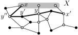
Figure 1: A graph with a vertex cover $S^{\prime\prime}$ (indicated in white) that is connected when all vertices in $X$ are identified into a single vertex. Shown are $x$, $x^{\prime}$,$y$,$y^{\prime}$,$y^{\prime\prime}$, and $P$ (indicated in bold) as used in the proof of Lemma 3.14.

Let $x$ and $x^{\prime}$ be in two distinct components in $G[S^{\prime\prime}]$, consider the shortest path $P$ from $x$ to $x^{\prime}$ in $G$. Refer to Figure 1 for a sketch of the situation. By this definition, $C_{x}\neq C_{x^{\prime}}$. Let $y$ be the first vertex in $P$ such that $y\in S^{\prime\prime}$ but $y\notin C_{x}$, let $y^{\prime}$ be the vertex on $P$ before $y$, observe that $y^{\prime}\notin S^{\prime\prime}$ since otherwise $y^{\prime}\in S^{\prime\prime}$ and $y^{\prime}\notin C_{x}$ which is a contradiction with the fact that $y$ is the first such vertex in $P$. Let $y^{\prime\prime}$ be the vertex on the path before $y^{\prime}$, such that $P=(x,\ldots,y^{\prime\prime},y^{\prime},y,\ldots,x^{\prime})$, where possibly $x=y^{\prime\prime}$ or $y=x^{\prime}$. Observe that $y^{\prime\prime}\in S^{\prime\prime}$ as otherwise edge $\{y^{\prime\prime},y^{\prime}\}$ is not covered, and therefore $y^{\prime\prime}\in C_{x}$ since $y$ is the first vertex on $P$ that is in $S^{\prime\prime}$ but not in $C_{x}$. Therefore, adding vertex $y^{\prime}$ to $S^{\prime\prime}$ will merge connected components $C_{x}$ and $C_{y}$, such that the number of connected components in $G[S^{\prime\prime}\cup\{y^{\prime}\}]$ is strictly smaller than the number of connected components in $G[S^{\prime\prime}]$. In total, we add less than $|X|$ vertices to $S^{\prime\prime}$ obtain a connected vertex cover $S^{\prime}$ and thus $|S^{\prime}|\leq|S|+|X|$.

We now prove the main result of this section.

Theorem 3.16.

For every $0<\varepsilon\leq 1$, Connected Vertex Cover parameterized by treewidth $\ell$ has a $(1+\varepsilon)$-approximate Turing Kernel with $\mathcal{O}(\big{(}\frac{\ell^{2}}{\varepsilon}\big{)}^{\big{\lceil}\frac{3+\varepsilon}{\varepsilon}\big{\rceil}})$ vertices.

Proof 3.17.

We will use the PSAKS for Connected Vertex Cover from Theorem 3.13. Recall that such a PSAKS consists of a reduction algorithm $R_{\mathcal{A}}$ together with a solution lifting algorithm $S_{\mathcal{A}}$. We will use the following claim.

Claim 7.

Given $0<\delta\leq 1$ and a connected graph $G$ with tree decomposition of width $\ell$, there is a polynomial-time algorithm to determine a $d$-approximate solution for CVC or correctly decide that $\mathrm{OPT}_{\text{CVC}}(G)>\frac{100\ell^{2}}{\delta}$, when given access to a $c$-approximate CVC-oracle that allows calls using graphs with at most $\mathcal{O}(\big{(}\frac{\ell^{2}}{\delta}\big{)}^{\big{\lceil}\frac{1+\delta}{\delta}\big{\rceil}})$ vertices, where $d=\min(c\cdot(1+\delta),2)$.

Using the fact that CVC is $2$-approximable in polynomial time [DBLP:journals/ipl/Savage82], obtain a $2$-approximate solution $\tilde{S}$ in $G$. If $|\tilde{S}|>200\ell^{2}/\delta$, return no and halt. Otherwise, continue by running $R_{\mathcal{A}}$ on $(G,|\tilde{S}|)$ to obtain $(G^{\prime},k^{\prime})$. Observe that $G^{\prime}$ has at most $\mathcal{O}(\big{(}\frac{\ell^{2}}{\delta}\big{)}^{\big{\lceil}\frac{1+\delta}{\delta}\big{\rceil}})$ many vertices. Apply the $c$-approximate oracle on $G^{\prime}$ to obtain CVC $S^{\prime}$ in $G^{\prime}$. Obtain an approximate solution $S$ in $G$ by using the solution lifting algorithm on $G^{\prime}$ and $S^{\prime}$. Output the smallest solution of $S$ and $\tilde{S}$, let this be $\hat{S}$. We show that this has the desired approximation factor, which requires an argument since the PSAKS works for $\text{CVC}^{\bot}$ instead of CVC (recall $\text{CVC}^{\bot}(G,k,S)=\min\{k+1,\text{CVC}(G,S)\}$). Observe that $|\hat{S}|\leq|\tilde{S}|$, by definition. Therefore, $|\hat{S}|\leq\text{CVC}^{\bot}(G,|\tilde{S}|,S)$. Thus

$$\frac{|\hat{S}|}{\mathrm{OPT}_{\text{CVC}}(G)}\leq\frac{\text{CVC}^{\bot}(G,|\tilde{S}|,S)}{\mathrm{OPT}_{\text{CVC}}(G)}\leq\frac{\text{CVC}^{\bot}(G,|\tilde{S}|,S)}{\mathrm{OPT}_{\text{CVC}^{\bot}}(G,|\tilde{S}|)}.$$

By correctness of the solution lifting algorithm, we get

$$\frac{\text{CVC}^{\bot}(G,|\tilde{S}|,S)}{\mathrm{OPT}_{\text{CVC}^{\bot}}(G,|\tilde{S}|)}\leq(1+\delta)\frac{\text{CVC}^{\bot}(G^{\prime},k^{\prime},S^{\prime})}{\mathrm{OPT}_{\text{CVC}^{\bot}}(G^{\prime},k^{\prime})}\leq(1+\delta)\frac{|S^{\prime}|}{\mathrm{OPT}_{\text{CVC}}(G^{\prime})}\leq c\cdot(1+\delta),$$

by correctness of the oracle.

Algorithm

The algorithm now proceeds as follows. Our goal is to find a subtree of $T$ for which on the one hand, the local optimum CVC is small enough to find an approximate solution using Claim 7, but also large enough to be able to (among other things) add the entire set $X_{t}$ to the solution, without introducing a too large error. Let $\delta:=\varepsilon/3$.

For any vertex $t\in V(T)$, let $G_{t}$ be the graph given by $G[V_{t}]$ after identifying all vertices from $X_{t}$ into a single vertex $z_{t}$. Apply Claim 7 to $G$, if it returns an approximate connected vertex cover of $G$, we are done. Otherwise, $\mathrm{OPT}_{\text{CVC}}(G)>\frac{100\ell^{2}}{\delta}$. We now aim to find a vertex $t$ such that Claim 7 returns an approximate solution in $G_{t}$ of size at least $\frac{10\ell}{\delta}$.

Claim 8.

There is a polynomial-time algorithm that, given $G$ with tree decomposition $\mathcal{T}$ of width $\ell$ such that $\mathrm{OPT}_{\text{CVC}}(G)>\frac{100\ell^{2}}{\delta}$, finds $t\in V(T)$ for which Claim 7 returns an approximate solution $S_{t}$ with $|S_{t}|\geq\frac{10\ell}{\delta}$, using calls to a $c$-approximate oracle of size at most $\mathcal{O}(\big{(}\frac{\ell^{2}}{\delta}\big{)}^{\big{\lceil}\frac{1+\delta}{\delta}\big{\rceil}})$.

Start with $t:=r$, note that since $\mathrm{OPT}_{\text{CVC}}(G)>\frac{100\ell^{2}}{\delta}$ and $G_{r}=G$, we have that $\mathrm{OPT}_{\text{CVC}}(G_{r})>\frac{100\ell^{2}}{\delta}$, where $r$ is the root of $T$. We search through the graph maintaining $\mathrm{OPT}_{\text{CVC}}(G_{t})>\frac{100\ell^{2}}{\delta}$. Let $t_{1},\ldots,t_{m}$ be the children of $t$, recall that we may assume $m\leq 2\ell+2$ by Theorem 2.3. For each $t_{i}$, apply Claim 7. Consider the following possibilities.

• There exists $i\in[m]$ such that the claim determines $\mathrm{OPT}_{\text{CVC}}(G_{t_{i}})>\frac{100\ell^{2}}{\delta}$, in this case, recurse with this $t_{i}$.

• There exists $i\in[m]$ such that the claim returns a $\min\{2,(1+\delta)\cdot c\}$-approximate solution $S_{t_{i}}$ of size at least $\frac{10\ell}{\delta}$ for CVC. In this case, return $t:=t_{i}$.

• Otherwise. Thus, for every $i\in[m]$, the algorithm returns a connected vertex cover $S_{i}$ of size at most $\frac{10\ell}{\delta}$ for CVC in $G_{t_{i}}$. Obtain a connected vertex cover $S_{i}^{\prime}$ of $G[V_{t_{i}}]$ of size at most $|S_{i}|+2(\ell+1)$ using Lemma 3.14. We will argue that in this case $CVC(G_{t})<\frac{55\ell^{2}}{\delta}$, which is a contradiction. We obtain a connected vertex cover of $G_{t}$ as follows. Let $\hat{S}_{t}:=\bigcup_{i\in[m]}(S_{i}^{\prime})\cup\{z_{t}\}$. Observe that $\hat{S}_{t}$ has size at most $(2\ell+2)\cdot\frac{13\ell}{\delta}+1\leq\frac{55\ell^{2}}{\delta}$. It is easy to observe that $\hat{S}_{t}$ is indeed a connected vertex cover of $G_{t}$.

Observe that from the steps above, we always get a connected vertex cover $S_{t}$ of $G_{t}$, that is a $(1+\delta)\cdot c$-approximation of $\mathrm{OPT}_{\text{CVC}}(G_{t})$ and has size at least $\frac{10\ell}{\delta}$.

Using Claim 8, we obtain a node $t$ and a connected vertex cover $S_{t}$ of $G_{t}$, that is a $\min\{(1+\delta)\cdot c,2\}$-approximation of $\mathrm{OPT}_{\text{CVC}}(G_{t})$ and has size at least $\frac{10\ell}{\delta}$. Use Lemma 3.14 to obtain a connected vertex cover $S_{t}^{\prime}$ of $G[V_{t}]$ of size at most $|S_{t}|+2(\ell+1)$, containing $X_{t}$.

We now obtain graph $G^{\prime}$ by removing all vertices in $V_{t}\setminus X_{t}$ from $G$ and then contracting all vertices in $X_{t}$ to a single vertex $z_{t}$. Let $\mathcal{T}^{\prime}$ to be a tree decomposition of $G^{\prime}$, one may obtain $\mathcal{T^{\prime}}$ by replacing occurrences of vertices in $V_{t}$ by $z_{t}$ in $\mathcal{T}$. Since $G^{\prime}$ is strictly smaller than $G$, we may use the algorithm described above to obtain a $c\cdot(1+\varepsilon)$-approximate solution $S^{\prime}$ for $\mathrm{OPT}_{\text{CVC}}(G^{\prime})$, using $\mathcal{T}^{\prime}$. Output $S:=S^{\prime}\cup S_{t}^{\prime}\setminus\{z_{t}\}$.

Correctness

We start by showing that $S$ is a connected vertex cover. Verify that it is indeed a vertex cover of $G$: any edge within $G^{\prime}$ is covered as $S^{\prime}\subseteq S$, any edge in $G_{t}$ is covered since $S_{t}^{\prime}\subseteq S$ and any other edge has at least one endpoint in $X_{t}\subseteq S$ and is thereby covered. It remains to verify that $G[S]$ is connected. Clearly, $G[V_{t}\cap S]$ is connected since it corresponds to $G[S_{t}^{\prime}]$. Let $\tilde{G}:=G-(V_{t}\setminus X_{t})$. We show that every connected component of $\tilde{G}[S]$ contains at least one vertex from $X_{t}$, such that the entire graph is connected as $X_{t}\subseteq S$ and the vertices in $X_{t}$ are in the same connected component as observed earlier. Suppose not, let $C$ be such a component not containing any vertex in $X_{t}$. Consider $G^{\prime}[S^{\prime}]$. Observe that $C$ is also a connected component of $G^{\prime}[S^{\prime}]$. Furthermore, vertex $z_{t}$ is not adjacent to any vertex in $C$, as otherwise there is an edge from some vertex in $C$ to some vertex in $X_{t}$ in $\tilde{G}$, since $X_{t}\subseteq S$ this contradicts that $C$ contains no vertex from $X_{t}$. Since $G^{\prime}$ is connected however, $z_{t}$ has an incident edge $\{z_{t},u\}$ for some $u\in V(G^{\prime})$ and thus $u\in S^{\prime}$ or $z_{t}\in S^{\prime}$. In both cases there is a vertex in $S^{\prime}$ that is not in connected component $C$, a contradiction with the assumption that $S^{\prime}$ is a connected vertex cover of $G^{\prime}$.

We now show that we indeed achieve the desired approximation factor.

Claim 9.

$|S|\leq c\cdot(1+\varepsilon)\cdot\mathrm{OPT}_{\text{CVC}}(G)$

Let $S^{*}$ be a minimum connected vertex cover of $G$. Assume for now $|S^{*}\cap V(G_{t})|\geq 4/\delta$.

$$|S| \leq|S_{t}^{\prime}|+|S^{\prime}|$$

$$\leq|S_{t}|+2(\ell+1)+c\cdot(1+\varepsilon)\mathrm{OPT}_{\text{CVC}}(G^{\prime})$$

Using $$|S_{t}|\geq\frac{10\ell}{\delta}$$

$$\leq|S_{t}|+\frac{\delta}{2}|S_{t}|+c\cdot(1+\varepsilon)\mathrm{OPT}_{\text{CVC}}(G^{\prime})$$

$$\leq c\cdot(1+\delta)(1+\delta/2)\mathrm{OPT}_{\text{CVC}}(G_{t})+c\cdot(1+\varepsilon)|(S^{*}\cap V(G^{\prime}))\cup\{z_{t}\}|$$

$$\leq c\cdot(1+\delta)(1+\delta/2)|(S^{*}\cap V(G_{t}))\cup\{z_{t}\}|+c\cdot(1+\varepsilon)|(S^{*}\cap V(G^{\prime}))\cup\{z_{t}\}|$$

$$\leq c\cdot(1+\delta)(1+\delta/2)(|S^{*}\cap V(G_{t})|+1)+c\cdot(1+\varepsilon)|(S^{*}\cap V(G^{\prime}))\cup\{z_{t}\}|$$

By assuming $$|S^{*}\cap V(G_{t})|\geq 4/\delta \delta=\varepsilon/3$$, and then using

$$\leq c\cdot(1+\delta)(1+\delta/2)(1+\delta/4)(|S^{*}\cap V(G_{t})|)+c\cdot(1+\varepsilon)|(S^{*}\cap V(G^{\prime}))\cup\{z_{t}\}|$$

$$\leq c\cdot(1+\varepsilon)(|S^{*}\cap V(G_{t})|)+c\cdot(1+\varepsilon)|(S^{*}\cap V(G^{\prime}))\cup\{z_{t}\}|$$

Observe that since $$G_{t} G^{\prime} S^{*} X_{t}$$ and are non-empty, must contain a vertex from

$$\leq c\cdot(1+\varepsilon)|S^{*}|=c\cdot(1+\varepsilon)\cdot\mathrm{OPT}_{\text{CVC}}(G).$$

It remains to observe that $|S^{*}\cap V(G_{t})|\geq 4/\delta$ is a reasonable assumption. Suppose not, then $\mathrm{OPT}_{\text{CVC}}(G_{t})\leq|S^{*}\cap V(G_{t})|+1\leq 4/\delta+1$. However, $S_{t}\geq\frac{10\ell}{\delta}\geq 2\cdot\mathrm{OPT}_{\text{CVC}}(G_{t})$, meaning that $S_{t}$ is not a $2$-approximation in $G_{t}$, which is a contradiction.

Having shown the correctness of the procedure, it remains to argue the size of this Turing kernel. Observe that the oracle is only used when applying Claim 7. As such, we may bound the size of the kernel by $\mathcal{O}(\big{(}\frac{\ell^{2}}{\delta}\big{)}^{\big{\lceil}\frac{1+\delta}{\delta}\big{\rceil}})=\mathcal{O}(\big{(}\frac{\ell^{2}}{\varepsilon}\big{)}^{\big{\lceil}\frac{3+\varepsilon}{\varepsilon}\big{\rceil}})$, recall that $\delta=\frac{\varepsilon}{3}$.

4 Meta result

In this section we will describe a wide range of graph problems for which approximate Turing kernels can be obtained. The problems we will consider satisfy certain additional constraints, such that the general strategy already described for the Vertex Cover problem can be applied. Informally speaking, we need the following requirements. First of all, the problems should behave nicely with respect to taking the disjoint union of graphs. Secondly, we want to look at what happens for induced subgraphs. We will only consider problems whose value cannot increase when taking an induced subgraph. Furthermore, we restrict how much the optimal value can decrease when taking an induced subgraph. Finally, we require existence of a PSAKS and an approximation algorithm for the problem. We use the following definitions.

Definition 4.1.

Let $\varphi\colon\mathbb{R}\times\mathbb{N}\to\mathbb{R}$ be a function. A $\varphi$-approximation algorithm for a problem $\mathcal{P}$ is a polynomial-time algorithm that, given an instance $G$ with tree decomposition $\mathcal{T}$ of width $\ell$, outputs a solution $S$ such that (for minimization problems) $\mathcal{P}(G,S)\leq\varphi(\mathrm{OPT}_{\mathcal{P}}(G),\ell)$, and (for maximization problems) $\varphi(\mathcal{P}(G,S),\ell)\geq\mathrm{OPT}_{\mathcal{P}}(G)$.

To illustrate this definition, observe that since Vertex Cover has a $2$-approximation, this same approximation algorithm serves as a $\varphi$-approximation with $\varphi(s,\ell)=2s$. We use the above definition to allow the approximation factor of the algorithm to depend on the size of the optimal solution and the treewidth of the considered graph.

We can now formally define our notion of a friendly problem.

Definition 4.2.

Let $\mathcal{P}$ be an optimization problem whose input is a graph. We will say that it is friendly if it satisfies the following conditions.

1. For all graphs $G$, $G_{1}$, and $G_{2}$ such that $G$ is the disjoint union of graphs $G_{1}$ and $G_{2}$, $\mathrm{OPT}_{\mathcal{P}}(G)=\mathrm{OPT}_{\mathcal{P}}(G_{1})+\mathrm{OPT}_{\mathcal{P}}(G_{2})$. In particular, if $S_{1}$ is a solution for $G_{1}$ and $S_{2}$ is a solution for $G_{2}$, then $S_{1}\cup S_{2}$ is a solution for $G$ and

   $$\mathcal{P}(G,S_{1}\cup S_{2})=\mathcal{P}(G_{1},S_{1})+\mathcal{P}(G_{2},S_{2}).$$

   In the other direction, given solution $S$ in $G$ it can efficiently be split into solutions $S_{1}$ in $G_{1}$ and $S_{2}$ in $G_{2}$ satisfying the above. For consistency, we require that the size of the optimal solution in the empty graph is zero.

2. There exists a non-decreasing polynomial function $f$ such that for all graphs $G$, for all $X\subseteq V(G)$:

   $$\mathrm{OPT}_{\mathcal{P}}(G)\leq\mathrm{OPT}_{\mathcal{P}}(G-X)+f(|X|)\text{, and }\mathrm{OPT}_{\mathcal{P}}(G-X)\leq\mathrm{OPT}_{\mathcal{P}}(G).$$

   In particular, for minimization problems there is a polynomial-time algorithm $\mathcal{A}$ that, given a solution $S^{\prime}$ in $G-X$, outputs a solution $S$ for $G$ such that $\mathcal{P}(G,S)\leq\mathcal{P}(G-X,S^{\prime})+f(|X|)$. For maximization problems we require that any solution $S$ for $G-X$ is also a solution for $G$ and $\mathcal{P}(G,S)=\mathcal{P}(G-X,S)$.

3. $\mathcal{P}^{\bot}$ parameterized by $k+\ell$, where $k$ is the solution value and $\ell$ is the treewidth, has a $(1+\delta)$-approximate kernel for all $\delta>0$, that has $h(\delta,k+\ell)$ vertices for some function $h$ that is polynomial in its second parameter.

4. $\mathcal{P}$ has a $\varphi$-approximation algorithm for some polynomial function $\varphi$ such that $\alpha\cdot\varphi(k,\ell)<\varphi(\alpha\cdot k,\ell)$ for all $\alpha>1$, and $\varphi$ is non-decreasing in its first parameter.

Observe that many well-known vertex subset problems fit in this framework. As an example, let us verify them for the