Reinforcement Learning assisted Quantum Optimization

Abstract

We propose a reinforcement learning (RL) scheme for feedback quantum control within the quantum approximate optimization algorithm (QAOA). QAOA requires a variational minimization for states constructed by applying a sequence of unitary operators, depending on parameters living in a highly dimensional space. We reformulate such a minimum search as a learning task, where a RL agent chooses the control parameters for the unitaries, given partial information on the system. We show that our RL scheme finds a policy converging to the optimal adiabatic solution for QAOA found by Mbeng et al. arXiv:1906.08948 for the translationally invariant quantum Ising chain. In presence of disorder, we show that our RL scheme allows the training part to be performed on small samples, and transferred successfully on larger systems.

Introduction — Quantum optimization and control are at the leading edge of current research in quantum computation Nielsen and Chuang (2000). Quantum Annealing (QA) Finnila et al. (1994); Kadowaki and Nishimori (1998); Brooke et al. (1999); Santoro et al. (2002); Santoro and Tosatti (2006), alias Adiabatic Quantum Computation (AQC) Farhi et al. (2001); Albash and Lidar (2018), is a promising quantum algorithm implemented Johnson et al. (2011) in present noisy intermediate-scale quantum devices Preskill (2018). More recently, the Quantum Approximate Optimization Algorithm (QAOA) Farhi et al. (2014) — a hybrid quantum-classical variational optimization scheme McClean et al. (2016) — has gained momentum  Lloyd (2018); Zhou et al. (2018); Mbeng, Glen B. and Fazio, Rosario and Santoro, Giuseppe E. (2019); Morales et al. (2019) and has been successfully realized in several experimental platforms Pagano et al. (2019); Arute et al. (2020).

In QA/AQC one constructs an interpolating Hamiltonian $\widehat{H}(s)=s\hat{H}_{z}+(1-s)\hat{H}_{x}$, where, e.g., for spin-1/2 systems $\hat{H}_{z}$ is the problem Hamiltonian whose ground state (GS) we are searching Lucas (2014) while $\hat{H}_{x}=-h\sum_{j}\hat{\sigma}^{x}_{j}$ is a transverse field term. An adiabatic dynamics is then attempted by slowly increasing $s(t)$ from $s(0)=0$ to $s(\tau)=1$ in a large annealing time $\tau$, starting from some easy-to-prepare initial state $|+\rangle$, the GS of $\hat{H}_{x}$. The difficulty is usually associated with the growing annealing time $\tau$ necessary when the system crosses a transition point, especially of first order Bapst et al. (2013).

QAOA, instead, uses a variational Ansatz of the form

$$|\psi_{\mathrm{P}}(\boldsymbol{\gamma},\boldsymbol{\beta})\rangle=\Big{(}\prod_{t}^{\mathrm{P}\leftarrow 1}\textrm{e}^{-i\beta_{t}\widehat{H}_{x}}\textrm{e}^{-i\gamma_{t}\widehat{H}_{z}}\Big{)}|+\rangle\;,$$ (1)

where $\boldsymbol{\gamma}=\gamma_{1},\dots,\gamma_{\mathrm{P}}$ and $\boldsymbol{\beta}=\beta_{1},\dots,\beta_{\mathrm{P}}$ are $2\mathrm{P}$ real parameters. The variational state $|\psi_{\mathrm{P}}(\boldsymbol{\gamma},\boldsymbol{\beta})\rangle$ is as a sequence of quantum gates, corresponding to 2$\mathrm{P}$ unitary evolution operators applied to the initial state, from right to left for increasing $t=1,\dots,\mathrm{P}$, each parameterized by control parameters $\gamma_{t}$ or $\beta_{t}$. The standard QAOA approach consists of a classical minimum search in such a $2\mathrm{P}$-dimensional energy landscape, which is in general not a trivial task McClean et al. (2018). Indeed, there are in general very many local minima in the QAOA-landscape, and local optimizations with random starting points produce irregular parameter sets $\left(\boldsymbol{\gamma}^{*},\boldsymbol{\beta}^{*}\right)$, hard to implement and sensitive to noise. To obtain stable and regular solutions $\left(\boldsymbol{\gamma}^{*},\boldsymbol{\beta}^{*}\right)$ that can be easily generalized to different values of $\mathrm{P}$ and implemented experimentally, it is necessary to employ iterative procedures during the minimum search Zhou et al. (2018); Pagano et al. (2019); Mbeng, Glen B. and Fazio, Rosario and Santoro, Giuseppe E. (2019). Interestingly, as discovered in Ref. Mbeng, Glen B. and Fazio, Rosario and Santoro, Giuseppe E. (2019) for quantum Ising chains, smooth regular optimal schedules for $\gamma_{t}$ and $\beta_{t}$ can be found, which are adiabatic in a digitized-QA/AQC Barends et al. (2016) context.

Figure 1: Scheme of: (a) a single step of Reinforcement Learning for QAOA; (b) the “episodes” loop in each $k$-th training “epoch”, with the “policy” and “state-value” neural networks $\Pi_{\theta_{k}}$ and $V^{\Pi}_{\theta^{\prime}_{k}}$.

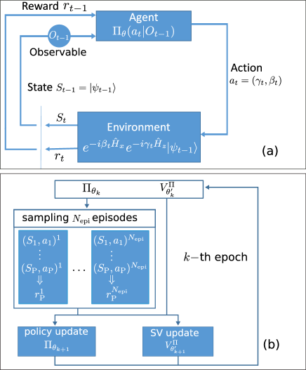
One might indeed reformulate the QAOA minimization as an optimal control process D’Alessandro (2007) in which one acts sequentially on the system in order to maximize a final reward. This reformulation seems particularly suited for Reinforcement Learning (RL) Sutton and Barto (2018); Kober et al. (2013); Mnih et al. (2013); Silver et al. (2017). As schematically represented in Fig. 1(a), at each discrete time step $t$ an “agent” is given some information, typically through measuring some observables $O_{t-1}$ on the state $S_{t-1}=|\psi_{t-1}\rangle$ of the system on which it acts (the “environment”). The agent then performs an action $a_{t}$ — here choosing the appropriate $(\gamma_{t},\beta_{t})$ and applying the corresponding unitaries to the state — obtaining a new state $S_{t}=|\psi_{t}\rangle$ and receiving a “reward” $r_{t}$, measuring the quality of the variational state constructed.

Several questions come to mind, which have not been addressed in the recent literature on RL applied to quantum problems Bukov et al. (2018); Fösel et al. (2018); August and Hernández-Lobato (2018); Khairy et al. (2019); Garcia-Saez and Riu (2019); Yao et al. (2020): i) is such RL-assisted QAOA able to “learn” optimal schedules? ii) Are the schedules found smooth in $t$? iii) How to dwell with the fact that getting information from $|\psi_{t}\rangle$ involves quantum measurements which destroy the state? iv) Are the strategies learned easily transferable to larger systems?

In this Letter we show, on the paradigmatic example of the transverse field Ising chain, that optimal strategies — well known in that case, see Ref. Mbeng, Glen B. and Fazio, Rosario and Santoro, Giuseppe E. (2019) — can be effectively learned with a simple Proximal Policy Optimization (PPO) algorithm Schulman et al. (2017) employing very small neural networks (NN). We show that RL automatically learns smooth control parameters, hence realizing an optimal controlled digitized-QA algorithm Mbeng, Glen B. and Fazio, Rosario and Santoro, Giuseppe E. (2019); Mbeng et al. (2019). By working with disordered quantum Ising chains we show that strategies “learned” on small samples can be successfully transferred to larger systems, hence alleviating the “measurement problem”: one can learn a strategy on a small problem which can be simulated on a computer, and implement it on a larger experimental setup Farhi et al. (2019).

RL-assisted QAOA — To test our scheme, we apply it to the transverse field Ising model (TFIM) in one dimension, where detailed QAOA results are already known Mbeng, Glen B. and Fazio, Rosario and Santoro, Giuseppe E. (2019). Specifically, we define the target Hamiltonian $\widehat{H}_{\mathrm{\scriptscriptstyle targ}}=\hat{H}_{z}+h\hat{H}_{x}$ with

$$\hat{H}_{z}=-\sum_{j=1}^{N}J_{j}\hat{\sigma}^{z}_{j}\hat{\sigma}^{z}_{j+1}\;,\hskip 14.22636pt\hat{H}_{x}=-\sum_{j}\hat{\sigma}^{x}_{j}\;.$$ (2)

We start considering the uniform TFIM, where $J_{j}=J$. The model has a paramagnetic ($h>J$) and a ferromagnetic ($h<J$) phase, separated by a $2^{\rm nd}$-order transition at $h=J$. The performance of QAOA on the uniform TFIM chain has been studied in detail in Refs. Wang et al. (2018); Mbeng, Glen B. and Fazio, Rosario and Santoro, Giuseppe E. (2019). Given a set of QAOA parameters $\left(\boldsymbol{\gamma},\boldsymbol{\beta}\right)$, we gauge the quality of the resulting state from the residual energy density

$$\epsilon_{\mathrm{P}}^{\rm res}\left(\boldsymbol{\gamma},\boldsymbol{\beta}\right)=\frac{E_{\mathrm{P}}\left(\boldsymbol{\gamma},\boldsymbol{\beta}\right)-E_{\min}}{E_{\max}-E_{\min}}\;,$$ (3)

where $E_{\mathrm{P}}\left(\boldsymbol{\gamma},\boldsymbol{\beta}\right)=\langle\psi_{\mathrm{P}}(\boldsymbol{\gamma},\boldsymbol{\beta})|\widehat{H}_{\mathrm{\scriptscriptstyle targ}}|\psi_{\mathrm{P}}(\boldsymbol{\gamma},\boldsymbol{\beta})\rangle$ is the variational energy, and $E_{\max}$ and $E_{\min}$ are the highest and lowest eigenvalues of the target Hamiltonian. Specifically, the results presented below will concern targeting the classical state for $h=0$, although the approach can be easily extended to the case with $h>0$. At $h=0$ the residual energy is bounded by the inequality Mbeng, Glen B. and Fazio, Rosario and Santoro, Giuseppe E. (2019)

$$\epsilon_{\mathrm{P}}^{\rm res}\left(\boldsymbol{\gamma},\boldsymbol{\beta}\right)\geq\left\{\begin{array}[]{ll}\frac{1}{2\mathrm{P}+2}&\hskip 5.69054pt\mbox{if}\hskip 5.69054pt2\mathrm{P}<N\vspace{2mm}\\ 0&\hskip 5.69054pt\mbox{if}\hskip 5.69054pt2\mathrm{P}\geq N\end{array}\right.\;,$$ (4)

which becomes an equality if and only if $(\boldsymbol{\gamma},\boldsymbol{\beta})$ are optimal QAOA parameters.

The key ingredients of the RL-assisted algorithm, as schematized in Fig. 1, are as follows.

State)

The state $S_{t}$ at time step $t=1,\dots,\mathrm{P}$ is encoded by the wave-function $|\psi_{t}\rangle$, defined iteratively as $|\psi_{t}\rangle=\textrm{e}^{-i\beta_{t}\widehat{H}_{x}}\textrm{e}^{-i\gamma_{t}\widehat{H}_{z}}|\psi_{t-1}\rangle$, with $|\psi_{0}\rangle=|+\rangle=\frac{1}{\sqrt{2^{N}}}\bigotimes_{i}\left(|\!\uparrow\rangle_{i}+|\!\downarrow\rangle_{i}\right)$. The agent has partial information through a number of observables $O_{t-1}$ measured on $|\psi_{t-1}\rangle$. Our choice (with $t-1\to t$) is

$$O_{t}=\big{\{}\langle\psi_{t}|\hat{\sigma}^{z}_{j}\hat{\sigma}^{z}_{j+1}|\psi_{t}\rangle,\langle\psi_{t}|\hat{\sigma}^{x}_{j}|\psi_{t}\rangle\big{\}}\;,$$ (5)

where a single value of $j$ is enough when translational invariance is respected.

Action)

The action $a_{t}$ at time $t$ corresponds to choosing $(\gamma_{t},\beta_{t})$. The conditional probability of $a_{t}$ given the observables $O_{t-1}$ — called “policy” in RL — is denoted by $\Pi_{\theta}(a_{t}|O_{t-1})$, where $\theta$ are the parameters of a Neural Network (NN) encoding. Our policy is stochastic, to help exploration: $\Pi_{\theta}(a|O)$ is chosen as a Gaussian distribution, whose mean and standard deviation are computed by the NN. From this, $a_{t}=(\gamma_{t},\beta_{t})$ is extracted.

Reward)

A reward $r_{t}$ is calculated at time $t$. In our present implementation, $r_{t=1,\dots,\mathrm{P}-1}=0$ and only $r_{\mathrm{P}}>0$. The final reward $r_{\mathrm{P}}=R(E_{\mathrm{P}})$ is associated to minimizing the final expectation value $E_{\mathrm{P}}=\langle\psi_{\mathrm{P}}|\widehat{H}_{\mathrm{\scriptscriptstyle targ}}|\psi_{\mathrm{P}}\rangle$. Here $R(E_{\mathrm{P}})$ is monotonically increasing when $E_{\mathrm{P}}$ decreases. Specifically, we take $R(E_{\mathrm{P}})=-E_{\mathrm{P}}$, but different non-linear choices have been tested.

Training)

The training process consists of a number $N_{\rm epo}$ of “epochs”, as sketched in Fig. 1(b). During each epoch the RL agent explores, with a fixed policy, the state-action trajectories for a certain number $N_{\rm epi}$ of “episodes”, each episode involving $\mathrm{P}$ steps $t=1,\dots,\mathrm{P}$. At the end of each epoch the policy is updated to favor trajectories with higher reward. The particular RL algorithm we used is the Proximal Policy Optimization (PPO) algorithm Schulman et al. (2017), from the OpenAI SpinningUp library Achiam (2018). PPO is an actor-critic algorithm where two independent NNs are used to parameterize the policy $\Pi_{\theta}(a_{t}|O_{t-1})$ and the state-value function Sutton and Barto (2018) $V_{\theta^{\prime}}^{\Pi}(O_{t})$. In our current implementation, $V_{\theta^{\prime}}^{\Pi}(O_{t})=\mathbb{E}^{\Pi}[r_{\mathrm{P}}]$ gives the expected reward that the system in a state with observables $O_{t}$ gets as it evolves with the policy $\Pi$. $V_{\theta^{\prime}}^{\Pi}(O_{t})$ is used to calculate the updates after each epoch Achiam (2018). In our numerical simulations, we used NNs with two fully-connected hidden layers of $32,16$ neurons, and linear-rectification (ReLu) activation function.

Results — In the RL training, the system is initially prepared in the state $|\psi_{0}\rangle=|+\rangle$, while the NNs for the policy and the state-value function are both initialized with random parameters. The agent is then trained for $N_{\rm epo}=1024$ epochs, each comprising $N_{\rm epi}=100$ episodes of $\mathrm{P}$ steps each. After training, we test the RL algorithm with $\sim 50$ runs.

Figure 2: (a) Residual energy density $\epsilon_{\mathrm{P}}^{\rm res}$, Eq. (3), vs $\mathrm{P}$. Full symbols: results from RL only; empty symbols: a local optimization (LO) supplements the RL actions (RL+LO); data are averaged over 50 test runs. The black dashed line is the lower bound of Eq. (4). (b) The schedule $s_{t}=\gamma_{t}/(\gamma_{t}+\beta_{t})$. Full blue lines denote $s_{t}$ learned after $N_{\rm epo}=1024$ epochs on a chain of $N=128$ sites; Dashed red lines, the RL+LO results; Black empty squares, the iterative LO smooth solution Mbeng, Glen B. and Fazio, Rosario and Santoro, Giuseppe E. (2019). The RL actions are in the basin of the same optimal minimum. Inset: same data for $N_{\rm epo}=128$ training epochs, where not all the LO optimized actions sets fall onto the iterative LO solution.

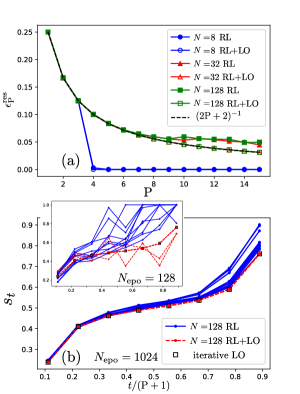
Fig. 2(a) shows the results obtained by the RL-trained policy. For $\mathrm{P}\leq 6$, the trained RL agent finds optimal QAOA parameters, saturating the bound for $\epsilon_{\mathrm{P}}^{\rm res}$ in Eq.(4). In particular, for small system sizes $N$, when $\mathrm{P}>N/2$, the agent finds the exact target ground state, and $\epsilon_{\mathrm{P}}^{\rm res}=0$. For longer episodes ($\mathrm{P}>6$), the residual energy deviates from the lower bound due to two factors: i) the longer the episode, the more difficult it is to learn the policy, as a larger number of training epochs are necessary to reach convergence; ii) since we are using a stochastic policy, the error due to the finite width of the action distributions is accumulated during an episode, leading to larger relative errors for longer trajectories. To cure this fact, we adopted the following strategy: we supplement the RL-trained policy with a final local optimization (LO) of the parameters $(\boldsymbol{\gamma},\boldsymbol{\beta})$, employing the Broyden-Fletcher-Goldfard-Shanno (BFGS) algorithm Nocedal and Wright (2006). This last step is computationally cheap, since the RL training brings the agent already close to a local minimum, provided $N_{\rm epo}$ is large enough. The residual energy data obtained in this way, denoted by RL+LO in Fig. 2(a), falls on top of the optimal curve $\epsilon_{\mathrm{P}}^{\rm res}=\frac{1}{2\mathrm{P}+2}$.

To visualize the action choices, we translate $\gamma_{t}$ and $\beta_{t}$ into the corresponding interpolation parameter $s_{t}$ which a Trotter-digitised QA/AQC would show, which for $h=0$ is given by: Mbeng, Glen B. and Fazio, Rosario and Santoro, Giuseppe E. (2019)

$$s_{t}=\frac{\gamma_{t}}{\gamma_{t}+\beta_{t}}\;.$$ (6)

Fig. 2(b) shows the interpolation parameter $s_{t}$ during an episode $t=1,\dots,\mathrm{P}$, for a chain of $N=128$ spins and $\mathrm{P}=8$. Different curves are obtained by repeating a test run of the same stochastic policy, trained for $N_{\rm epo}=1024$ epochs. The parameters obtained through the RL policy are smooth, and different tests result in similar s-shaped profiles for $s_{t}$. When a final local minimization is added, the curves for $s_{t}$ coalesce and coincides with the smooth optimal schedule obtained in Ref. Mbeng, Glen B. and Fazio, Rosario and Santoro, Giuseppe E. (2019) through an independent iterative local optimization strategy. When the training is at an early stage, i.e. the number of epochs is small, see inset of Fig. 2(b), the profiles $s_{t}$ are more irregular and do not fall all in the same smooth minimum upon performing the LO (see the three dashed red lines).

Next, we turn to the random TFIM case. Here, for each chain length $N$ we fix a given disorder instance $\{J_{j}\}_{j=1,\dots,N}$ with $J_{j}\in[0,1]$, both for the training and the test of the RL policy. Since translational invariance is now lost, one would naively imagine that the relevant observables $O_{t}$ in Eq. (5) would involve a list of $2N$ measurements. However, our experience has taught us that we can efficiently go on with a reduced list comprising only the two Hamiltonian terms, $O_{t}=\big{\{}\langle\psi_{t}|\hat{H}_{z}|\psi_{t}\rangle,\langle\psi_{t}|\hat{H}_{x}|\psi_{t}\rangle\big{\}}$, hence chain-averaged quantities. All the parameters involved in training the NNs are fixed as in the uniform TFIM case.

Fig. 3(a) shows the residual energy $\epsilon_{\mathrm{P}}^{\rm res}$ vs $\mathrm{P}$ obtained from the bare RL (full symbols) and from RL followed by a local optimization (RL+LO, empty symbols). The local optimization significantly improves the quality for large $\mathrm{P}\geq 10$. A detailed study of the behaviour of $\epsilon_{\mathrm{P}}^{\rm res}$ for large $\mathrm{P}$ and a comparison with the results obtained Caneva et al. (2007) by a linear-QA/AQC scheme, with $s(t)=t/\tau$, is left to a future study.

Figure 3: (a) Residual energy, Eq. (3), vs $\mathrm{P}$ for a single instance of the random TFIM: comparison between bare RL and RL followed by local optimization (LO) results (RL+LO). (b) The optimized $s_{t}$ obtained with different procedures. Empty squares: the iterative LO process of Ref. Mbeng, Glen B. and Fazio, Rosario and Santoro, Giuseppe E. (2019); Blue circles: RL+LO performed directly on a $N=128$ chain; Gray lines: $\mathrm{RL}_{\scriptscriptstyle N=8}\!+\!\mathrm{LO}_{\scriptscriptstyle N=128}$, i.e., training of a $N=8$ chain used as Ansatz for LO of the $N=128$ chain.

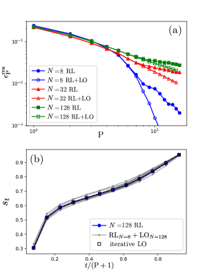
Fig. 3(b) shows the optimal parameter $s_{t}=\gamma_{t}/(\gamma_{t}+\beta_{t})$ found by the RL+LO method, compared to the $s_{t}$ constructed with the iterative optimization strategy described in Ref. Mbeng, Glen B. and Fazio, Rosario and Santoro, Giuseppe E. (2019): the agreement between the two is remarkable, showing that the RL-assisted QAOA effectively “learns” smooth action trajectories.

The most remarkable fact, however, is shown by the series of grey lines present in Fig. 3(b). These are obtained by training the RL agent on a much smaller instance with $N=8$ sites, and transferring the RL-policy to the larger (and different) disorder instance with $N=128$, followed by local optimizations of the learned parameters. These results show a large transferability of the RL policies, which we have verified to hold even in the absence of the final LO. This suggests the following way-out from the “measurement problem” involved in the construction of the state observables $O_{t}$. Indeed, in an experimental implementation of RL-assisted QAOA, the RL agent could observe a small system, efficiently simulated on a classical hardware, and then use the learned actions to evolve the larger experimental system. This reduces drastically the number of measurements to be performed and allows to test RL-assisted QAOA on physical quantum platforms.

Conclusions — In this Letter we have shown that the optimal QAOA strategies well known for the TFIM Mbeng, Glen B. and Fazio, Rosario and Santoro, Giuseppe E. (2019) can be effectively learned with a simple PPO-algorithm Schulman et al. (2017) employing rather small NNs. The observables measured on a state, referring to the two competing terms in the Hamiltonian and providing information to the “agent”, seem to be effective in the learning process. We have shown that RL learns smooth control parameters, hence realizing an RL-assisted feedback Quantum Control for the schedule $s(t)$ of a digitized QA/AQC algorithm Mbeng, Glen B. and Fazio, Rosario and Santoro, Giuseppe E. (2019), in absence of any spectral information. By working with disordered quantum Ising chains we showed that strategies “learned” on small samples can be successfully transferred to larger systems, hence alleviating the “measurement problem”: one can learn a strategy on a small problem simulated on a computer, and implement it on a larger experimental setup.

A discussion of previous RL-work on quantum systems is here appropriate. RL as a tool for quantum control and quantum-error-correction has been investigated in Refs. Bukov et al. (2018); Fösel et al. (2018). Regarding applications to QAOA, Refs. August and Hernández-Lobato (2018); Khairy et al. (2019); Yao et al. (2020) have all formulated RL strategies to learn optimal variational parameters $(\boldsymbol{\gamma},\boldsymbol{\beta})$. While sharing similar RL tools, their approach is markedly different from ours: they identify the RL “state” with the whole set of QAOA parameters. The agent has no access to the internal quantum state, and no information on the evolution process can be exploited in the optimization. In this way, the issue of measuring the intermediate quantum state is bypassed. This choice, however, reduces RL to a heuristic optimization which forfeits one of the most relevant feature of the RL framework: The possibility to drive the process with a step-by-step evolution. An alternative proposal, closer to ours in methods but tackling different physical questions, has recently appeared in Ref. Garcia-Saez and Riu (2019).

Concerning future developments, we mention possible improvements of the “measurement problem”. One possibility is to introduce ancillary bits to provide intermediate information to the RL agent without destroying the state of the system, in a way similar to Ref. Fösel et al. (2018). A possible alternative is to perform weak measurements Vitale et al. (2019). A second issue is the sensitivity to noise: preliminary results show that noise in the initial state preparation does not harm the ability to learn the correct strategies. Finally, the application to other models is worth pursuing: preliminary results on the fully-connected p-spin Ising ferromagnet are encouraging.

We thank R. Fazio for stimulating discussions. Research was partly supported by EU Horizon 2020 under ERC-ULTRADISS, Grant Agreement No. 834402. GES acknowledges that his research has been conducted within the framework of the Trieste Institute for Theoretical Quantum Technologies (TQT).

References

- Nielsen and Chuang (2000) M. Nielsen and I. L. Chuang, Quantum Computation and Quantum Information (Cambridge University Press, 2000).
- Finnila et al. (1994) A. B. Finnila, M. A. Gomez, C. Sebenik, C. Stenson, and J. D. Doll, Chem. Phys. Lett. 219, 343 (1994).
- Kadowaki and Nishimori (1998) T. Kadowaki and H. Nishimori, Phys. Rev. E 58, 5355 (1998).
- Brooke et al. (1999) J. Brooke, D. Bitko, T. F. Rosenbaum, and G. Aeppli, Science 284, 779 (1999).
- Santoro et al. (2002) G. E. Santoro, R. Martoňák, E. Tosatti, and R. Car, Science 295, 2427 (2002).
- Santoro and Tosatti (2006) G. E. Santoro and E. Tosatti, J. Phys. A: Math. Gen. 39, R393 (2006).
- Farhi et al. (2001) E. Farhi, J. Goldstone, S. Gutmann, J. Lapan, A. Lundgren, and D. Preda, Science 292, 472 (2001).
- Albash and Lidar (2018) T. Albash and D. A. Lidar, Rev. Mod. Phys. 90, 015002 (2018).
- Johnson et al. (2011) M. W. Johnson et al., Nature 473, 194 (2011).
- Preskill (2018) J. Preskill, Quantum 2, 79 (2018), ISSN 2521-327X.
- Farhi et al. (2014) E. Farhi, J. Goldstone, and S. Gutmann, arXiv e-prints arXiv:1411.4028 (2014), eprint 1411.4028.
- McClean et al. (2016) J. R. McClean, J. Romero, R. Babbush, and A. Aspuru-Guzik, New Journal of Physics 18, 023023 (2016).
- Lloyd (2018) S. Lloyd, arXiv e-prints arXiv:1812.11075 (2018), eprint 1812.11075.
- Zhou et al. (2018) L. Zhou, S.-T. Wang, S. Choi, H. Pichler, and M. D. Lukin, arXiv e-prints arXiv:1812.01041 (2018), eprint 1812.01041.
- Mbeng, Glen B. and Fazio, Rosario and Santoro, Giuseppe E. (2019) Mbeng, Glen B. and Fazio, Rosario and Santoro, Giuseppe E., arXiv e-prints arXiv:1906.08948 (2019), eprint 1906.08948.
- Morales et al. (2019) M. E. S. Morales, J. Biamonte, and Z. Zimborás (2019), eprint 1909.03123.
- Pagano et al. (2019) G. Pagano, A. Bapat, P. Becker, K. S. Collins, A. De, P. W. Hess, H. B. Kaplan, A. Kyprianidis, W. L. Tan, C. Baldwin, et al., arXiv e-prints arXiv:1906.02700 (2019), eprint 1906.02700.
- Arute et al. (2020) F. Arute, K. Arya, R. Babbush, D. Bacon, J. C. Bardin, R. Barends, S. Boixo, M. Broughton, B. B. Buckley, D. A. Buell, et al. (2020), eprint 2004.04197.
- Lucas (2014) A. Lucas, Frontiers in Physics 2, 5 (2014).
- Bapst et al. (2013) V. Bapst, L. Foini, F. Krzakala, G. Semerjian, and F. Zamponi, Physics Reports 523, 127 (2013).
- McClean et al. (2018) J. R. McClean, S. Boixo, V. N. Smelyanskiy, R. Babbush, and H. Neven, Nature Communications 9, 4812 (2018), ISSN 2041-1723.
- Barends et al. (2016) R. Barends, A. Shabani, L. Lamata, J. Kelly, A. Mezzacapo, U. L. Heras, R. Babbush, A. G. Fowler, B. Campbell, Y. Chen, et al., Nature 534, 222 EP (2016).
- D’Alessandro (2007) D. D’Alessandro, Introduction to quantum control and dynamics (Chapman and Hall/CRC, 2007).
- Sutton and Barto (2018) R. S. Sutton and A. G. Barto, Reinforcement Learningi, An Introduction (The MIT Press, 2018), 2nd ed.
- Kober et al. (2013) J. Kober, J. A. Bagnell, and J. Peters, The International Journal of Robotics Research 32, 1238 (2013).
- Mnih et al. (2013) V. Mnih, K. Kavukcuoglu, D. Silver, A. Graves, I. Antonoglou, D. Wierstra, and M. Riedmiller, arXiv preprint arXiv:1312.5602 (2013).
- Silver et al. (2017) D. Silver, J. Schrittwieser, K. Simonyan, I. Antonoglou, A. Huang, A. Guez, T. Hubert, L. Baker, M. Lai, A. Bolton, et al., Nature 550, 354 (2017).
- Bukov et al. (2018) M. Bukov, A. G. R. Day, D. Sels, P. Weinberg, A. Polkovnikov, and P. Mehta, Phys. Rev. X 8, 031086 (2018).
- Fösel et al. (2018) T. Fösel, P. Tighineanu, T. Weiss, and F. Marquardt, Phys. Rev. X 8, 031084 (2018).
- August and Hernández-Lobato (2018) M. August and J. M. Hernández-Lobato (2018), eprint 1802.04063.
- Khairy et al. (2019) S. Khairy, R. Shaydulin, L. Cincio, Y. Alexeev, and P. Balaprakash (2019), eprint 1911.11071.
- Garcia-Saez and Riu (2019) A. Garcia-Saez and J. Riu (2019), eprint 1911.09682.
- Yao et al. (2020) J. Yao, M. Bukov, and L. Lin (2020), eprint 2002.01068.
- Schulman et al. (2017) J. Schulman, F. Wolski, P. Dhariwal, A. Radford, and O. Klimov, CoRR abs/1707.06347 (2017), eprint 1707.06347.
- Mbeng et al. (2019) G. B. Mbeng, R. Fazio, and G. E. Santoro, Optimal quantum control with digitized quantum annealing (2019), eprint 1911.12259.
- Farhi et al. (2019) E. Farhi, J. Goldstone, S. Gutmann, and L. Zhou, The quantum approximate optimization algorithm and the sherrington-kirkpatrick model at infinite size (2019), eprint 1910.08187.
- Wang et al. (2018) Z. Wang, S. Hadfield, Z. Jiang, and E. G. Rieffel, Phys. Rev. A 97, 022304 (2018).
- Achiam (2018) J. Achiam (2018).
- Nocedal and Wright (2006) J. Nocedal and S. Wright, Numerical optimization (Springer Science & Business Media, 2006).
- Caneva et al. (2007) T. Caneva, R. Fazio, and G. E. Santoro, Phys. Rev. B 76, 144427 (2007).
- Vitale et al. (2019) V. Vitale, G. De Filippis, A. de Candia, A. Tagliacozzo, V. Cataudella, and P. Lucignano, Scientific Reports 9, 13624 (2019).