Supplementary Materials
CLUE: Exact maximal reduction of kinetic models
by constrained lumping of differential equations

This document is structured as follows:

• In Section I, we will prove the correctness and termination the algorithms presented in the paper.

• In Section II, we reprove the criterion for lumping in terms of the Jacobian of the system (Li and Rabitz, 1991, Section 2) for the sake of completeness.

• In Section III, we present a complexity analysis of our algorithms and compare it with the complexity of ERODE.

• In Section IV, we discuss the application of CLUE to a cartilage breakdown model in (Proctor et al., 2014).

• In Section V, we compare the performance of our implementations Algorithms 2 and Algorithm 3.

Remark.

In the present paper, we have focused on exact maximal reduction for ODEs with a polynomial right-hand side because our examples are in this class. However, all of our algorithms can be immediately applied to other kinds of systems, such as discrete-time polynomial systems (e.g. $\mathbf{x}_{n+1}=\mathbf{f}(\mathbf{x}_{n})$).

I Proofs of correctness and termination of algorithms

For the convenience of the reader while navigating between the main paper and the Supplementary materials, we recall:

Algorithm 1 Simplified algorithm for finding a constrained lumping of the smallest possible dimension

Input

a system $\dot{\mathbf{x}}=\mathbf{f}(\mathbf{x})$ of $n$ ODEs with a polynomial right-hand side and an $s\times n$ matrix $A$ over field $\mathbb{K}$ of rank $s>0$;

Output

a matrix $L$ such that $\mathbf{y}:=L\mathbf{x}$ is a constrained lumping with observables $A\mathbf{x}$ of smallest possible dimension.

1. Compute $J(\mathbf{x})$, the Jacobian matrix of $\mathbf{f}(\mathbf{x})$.

2. Represent $J(\mathbf{x})$ as $J_{1}m_{1}+\ldots+J_{N}m_{N}$, where $m_{1},\ldots,m_{N}$ are distinct monomials in $\mathbf{x}$, and $J_{1},\ldots,J_{N}$ are nonzero matrices over $\mathbb{R}$.

3. Set $L:=A$.

4. Repeat

   1. for every $M$ in $J_{1},\ldots,J_{N}$ and row $r$ of $L$, if $rM$ does not belong to the row space of $L$, append $rM$ to $L$.

   2. if nothing has been appended in the previous step, exit the repeat loop and go to (Step 5).

5. Return $L$.

Algorithm 2 Finding the smallest invariant subspace
(to be used instead of (Step 4) of Algorithm 1 for $A=L$, $\ell=N$, and $M_{i}=J_{i}$ for $1\leqslant i\leqslant\ell$)

Input

an $s\times n$ matrix $A$ over field $\mathbb{K}$ and a list $M_{1},\ldots,M_{\ell}$ of $n\times n$ matrices over $\mathbb{K}$;

Output

an $r\times n$ matrix $L$ over $\mathbb{K}$ such that

• the row span of $A$ is contained in the row span of $L$.

• for every $1\leqslant i\leqslant\ell$, the row span of span of $LM_{i}$ is contained in the row span of $L$;

• $r$ is the smallest possible.

1. Let $L$ be the reduced row echelon form of $A$.

2. Set $P$ be the set of indices of the pivot columns of $L$.

3. While $P\neq\varnothing$ do

   1. For every $j\in P$ and every $1\leqslant i\leqslant\ell$

      1. Let $v$ be the row in $L$ with the index of the pivot being $j$.

      2. Reduce $vM_{i}$ with respect to $L$. If the result is not zero, append it as a new row to $L$.

      3. Reduce other rows with respect the new one in order to bring $L$ into the reduced row echelon form.

   2. Let $\widetilde{P}$ be the set of indices of the pivot columns of $L$.

   3. Set $P:=\widetilde{P}\setminus P$.

4. Return $L$.

Algorithm 3 Finding the smallest invariant subspace (modular)
(to be used instead of (Step 4) of Algorithm 1 for $A=L$, $\ell=N$, and $M_{i}=J_{i}$ for $1\leqslant i\leqslant\ell$)

Input

$s\times n$ matrix $A$ and a list $M_{1},\ldots,M_{\ell}$ of $n\times n$ matrices over $\mathbb{Q}$;

Output

an $r\times n$ matrix $L$ over $\mathbb{Q}$ such that:

• the row span of $A$ is contained in the row span of $L$.

• for every $1\leqslant i\leqslant\ell$, the row span of $LM_{i}$ is contained in the row span of $L$;

• $r$ is the smallest possible.

1. Repeat the following

   1. Pick a prime number $p$ that does not divide any of the denominators in $A,M_{1},\ldots,M_{\ell}$ and has not been chosen before.

   2. Compute the reductions $\widetilde{A},\widetilde{M}_{1},\ldots,\widetilde{M}_{\ell}$ modulo $p$.

   3. Run Algorithm 2 on $\widetilde{A},\widetilde{M}_{1},\ldots,\widetilde{M}_{\ell}$ as matrices over $\mathbb{F}_{p}$ and denote the result by $\widetilde{L}$.

   4. Apply the rational reconstruction algorithm ((von zur Garthen and Gerhard, 2013, § 5.10), (Wang et al., 1982)) to construct a matrix $L$ over $\mathbb{Q}$ such that the reduction of $L$ mod $p$ equals $\widetilde{L}$.

   5. Check whether the row span of $L$ contains the row span of $L$ and is invariant under $M_{1},\ldots,M_{\ell}$. If yes, exit the loop.

2. Return the matrix $L$ from step (Step 1)(d) of the last iteration of the loop.

Notation I.1.

• $\operatorname{Mat}_{m,n}(\mathbb{K})$ denotes the space of $m\times n$ matrices over a field $\mathbb{K}$.

• For $M\in\operatorname{Mat}_{m,n}(\mathbb{K})$, $\operatorname{rspan}_{\mathbb{K}}(M)$ is the row span of $M$ over $\mathbb{K}$.

Lemma I.1 is used by Algorithm 1 to pass from the invariance under the Jacobian to the invariance under a finite set of constant matrices.

Lemma I.1.

Let $M(\mathbf{x})\in\operatorname{Mat}_{n,n}(\mathbb{K}[\mathbf{x}])$, where $\mathbf{x}=(x_{1},\ldots,x_{r})$ and $\operatorname{char}\mathbb{K}=0$. We write $M(\mathbf{x})=M_{1}m_{1}+\ldots+M_{N}m_{M}$ so that $M_{1},\ldots,M_{N}\in\operatorname{Mat}_{n,n}(\mathbb{K})$ and $m_{1},\ldots,m_{N}$ are distinct monomials in $\mathbf{x}$. Then, for a vector subspace $V\subset\mathbb{K}^{n}$, the following are equivalent:

1. $V$ is invariant under $M(\mathbf{x}^{\ast})$ for every $\mathbf{x}^{\ast}\in\mathbb{K}^{r}$;

2. $V$ is invariant under $M_{i}$ for every $1\leqslant i\leqslant N$.

Proof.

Assume that $V$ is invariant under $M_{1},\ldots,M_{N}$. Since, for every $\mathbf{x}^{\ast}\in\mathbb{K}^{r}$, $M(\mathbf{x}^{\ast})$ is an $\mathbb{K}$-linear combination of $M_{1},\ldots,M_{N}$, $V$ is invariant under $M(\mathbf{x}^{\ast})$ as well.

Assume that $V$ is invariant under $M(\mathbf{x}^{\ast})$ for every $\mathbf{x}^{\ast}\in\mathbb{K}^{r}$. Consider $v\in V$. Since for all $\mathbf{x}^{\ast}\in\mathbb{K}^{r}$, $M(\mathbf{x}^{\ast})v\in V$, for every $1\leqslant i\leqslant r$, $\frac{\partial M}{\partial x_{i}}(\mathbf{x}^{\ast})v\in V$ as well. Consider one of $M_{1},\ldots,M_{N}$, say $M_{1}$. Let $m_{1}=x_{1}^{d_{1}}\ldots x_{r}^{d_{r}}$. Iterating the argument with derivative, we obtain

$$\forall\mathbf{x}^{\ast}\in\mathbb{K}^{r}\ \ \frac{\partial^{d_{1}+\ldots+d_{r}}M}{\partial x_{1}^{d_{1}}\ldots\partial x_{r}^{d_{r}}}(\mathbf{x}^{\ast})v\in V.$$

Taking $\mathbf{x}^{\ast}=\mathbf{0}$, we deduce that $M_{1}v\in V$. ∎

Remark I.1.

A different approach to replacing the Jacobian with a finite set of constant matrices was suggested in (Li and Rabitz, 1989, Sect. 3(A)):

1. Write the Jacobian $J(\mathbf{x})=\sum a_{ij}(\mathbf{x})E_{ij}$, where $E_{ij}$ is the matrix with one in the $(i,j)$-th cell and zeroes everywhere else;

2. Combine together summands with proportional $a_{ij}(\mathbf{x})$ obtaining a representation $J(\mathbf{x})=\sum b_{j}(\mathbf{x})B_{j}$ with constant $B_{j}$;

3. Return $B_{j}$’s.

Consider the system

$$\begin{cases}\dot{x}_{1}=(x_{2}+x_{3})^{2}+(x_{2}+x_{4})^{2},\\ \dot{x}_{2}=\dot{x}_{3}=\dot{x}_{4}=0\end{cases}$$

with the observable $x_{1}$. Then the procedure from (Li and Rabitz, 1989, Section 3(A)) will lead to the following decomposition

$$J(\mathbf{x})=2(2x_{2}+x_{3}+x_{4})E_{12}+2(x_{2}+x_{3})E_{13}+2(x_{2}+x_{4})E_{14}.$$

The smallest subspace containing $(1,0,0,0)$ and right-invariant under $E_{12},E_{13},E_{14}$ is the whole space, so this approach will not produce a nontrivial lumping. On the other hand, using Lemma I.1, we arrive at

$$J(\mathbf{x})=2x_{2}(2E_{12}+E_{13}+E_{14})+2x_{3}(E_{12}+E_{13})+2x_{4}(E_{12}+E_{14}).$$

The matrices $2E_{12}+E_{13}+E_{14},E_{12}+E_{13}$, and $E_{12}+E_{14}$ have a common proper invariant subspace containing $(1,0,0,0)$, and this yields a nontrivial lumping:

$$y_{1}=x_{1},\quad y_{2}=x_{2}+x_{3},\quad y_{3}=x_{2}+x_{4}.$$

Proposition I.1.

Algorithm 2 is correct.

Proof.

Bringing a matrix to the reduced row echelon form does not change the row span, and adding extra rows might only enlarge it, so the row span of the output of Algorithm 2 contains the row span of $A$.

Now we will show that the row span of the output of the algorithm is invariant under $M_{1},\ldots,M_{N}$. We denote the values of $L$ and $P$ before the $i$-th iteration of the while loop (Step 3) by $L_{i}$ and $P_{i}$, respectively. We set $L_{0}$ and $P$ to be the $0\times n$ matrix and $\varnothing$, respectively. We will show by induction on $k$ that, for every $k\geqslant 0$ and every $1\leqslant i\leqslant\ell$, we have

$$\operatorname{rspan}_{\mathbb{K}}(L_{k}M_{i})\subset\operatorname{rspan}_{\mathbb{K}}(L_{k+1}).$$ (1)

The case $k=0$ is true. Assume that the statement is true for all numbers less than some $k>0$. Let $L_{+}$ be the matrix consisting of the rows of $L_{k}$ with the pivot columns in $P_{k}$, and let $L_{-}$ be the matrix consisting of the remaining rows. Fix $1\leqslant i\leqslant\ell$. Then $\operatorname{rspan}_{\mathbb{K}}(L_{+}M_{i})\subset\operatorname{rspan}_{\mathbb{K}}L_{k+1}$ because the rows of $L_{+}$ will be processed in the next iteration of the while loop. By the construction, $\operatorname{rspan}_{\mathbb{K}}L_{k-1}\subset\operatorname{rspan}_{\mathbb{K}}L_{k}$. The rows of $L_{k-1}$ and $L_{+}$ are linearly independent because they form a (nonreduced) row echelon form after permuting rows and columns. Therefore, $\operatorname{rspan}_{\mathbb{K}}L_{k}=\operatorname{rspan}_{\mathbb{K}}L_{+}+\operatorname{rspan}_{\mathbb{K}}L_{k-1}$. This implies

$$\operatorname{rspan}_{\mathbb{K}}(L_{-}M_{i})\subset\operatorname{rspan}_{\mathbb{K}}(L_{+}M_{i})+\operatorname{rspan}_{\mathbb{K}}(L_{k-1}M_{i}).$$

The inductive hypothesis implies that

$$\operatorname{rspan}_{\mathbb{K}}(L_{-}M_{i})\subset\operatorname{rspan}_{\mathbb{K}}(L_{+}M_{i})+\operatorname{rspan}_{\mathbb{K}}L_{k}\subset\operatorname{rspan}_{\mathbb{K}}L_{k+1}.$$

Therefore, $\operatorname{rspan}_{\mathbb{K}}(L_{k}M_{i})\subset\operatorname{rspan}_{\mathbb{K}}L_{k+1}$.

Assume that there were $N$ iterations of the while loop. Then we consider one extra iteration. Since $P=\varnothing$, this iteration will not do anything, so $L_{N+2}=L_{N+1}$. Therefore, $\operatorname{rspan}_{\mathbb{K}}(L_{N+1}M_{i})\subset\operatorname{rspan}_{\mathbb{K}}(L_{N+1})$ for every $1\leqslant i\leqslant\ell$ due to (1). This implies that $\operatorname{rspan}_{\mathbb{K}}$ of the output of the algorithm is invariant under $M_{1},\ldots,M_{\ell}$.

To prove the minimality of $r$, consider $V$, the smallest subspace of $\mathbb{K}^{n}$ invariant under $M_{1},\ldots,M_{\ell}$ and containing the rows of the input matrix $A$. We will show by induction on $i$ that $\operatorname{rspan}_{\mathbb{K}}(L_{i})\subset V$. Since $\operatorname{rspan}_{\mathbb{K}}(L_{1})=\operatorname{rspan}_{\mathbb{K}}A$, $\operatorname{rspan}_{\mathbb{K}}(L_{1})\subset V$. Assume that the statement is true for some $i\geqslant 1$. At the $i$-th iteration of the while loop, we consider vectors of the form $vM_{i}$, where $v\in\operatorname{rspan}_{\mathbb{K}}(L_{i})$. Since $v\in V$ and $V$ is $M_{i}$-invariant, these vectors also belong to $V$. Consequent computation of the row echelon form does not change the row span. Hence, the row span of the output is invariant under $M_{1},\ldots,M_{\ell}$ and contained in $V$, so it coincides with $V$. This proves the minimality of $r$. ∎

The following lemma is used in Proposition I.2 for showing the correctness and termination of Algorithm 3.

Lemma I.2.

Let $A\in\operatorname{Mat}_{s,n}(\mathbb{Q})$, $M_{1},\ldots,M_{\ell}\in\operatorname{Mat}_{n,n}(\mathbb{Q})$ and $L$ the result of applying Algorithm 2 to these matrices. For every prime number $p$ that does not divide the denominators of the entries of $A,M_{1},\ldots,M_{\ell}$, we denote the result of applying Algorithm 2 to the reductions of these matrices modulo $p$ by $L_{p}^{\ast}$. Then

1. for all but finitely many primes, $L^{\ast}_{p}$ is equal to $L$ modulo $p$;

2. the number of rows in $L_{p}^{\ast}$ does not exceed the number of rows in $L$.

Proof.

To show (1), consider the run of Algorithm 2 on $A,M_{1},\ldots,M_{\ell}$. The operations performed with the matrix entries in the algorithm are arithmetic operations and checking for nullity. There is a finite list of nonzero rational numbers $q_{1},\ldots,q_{N}$ checked for nullity in the algorithm. Consider a prime number $p$ such that the reductions of $q_{1},\ldots,q_{N}$ modulo $p$ are defined and not zero. Since the arithmetic operations commute with reducing modulo $p$ and we have chosen $p$ so that all nullity checks will also commute with reduction modulo $p$, the result of the algorithm modulo $p$, that is $L_{p}^{\ast}$, will be equal to the reduction of $L$ modulo $p$.

We now show (1). The number of rows in $L$ is the dimension of the space generated by the rows of $A$ and their images under all possible products of $M_{1},\ldots,M_{\ell}$. Consider the $\infty\times n$ matrix $R$ formed from the matrices of the form $AX$, where $X$ ranges over all possible products of $M_{1},\ldots,M_{\ell}$, stacked on top of each other. Let $R_{p}$ be the reduction of $R$ modulo $p$. For every integer $r$, having rank at most $r$ can be expressed as a system of polynomial conditions in the matrix entries (that is, all $(r+1)\times(r+1)$ minors are zero). Therefore, $\operatorname{rank}R_{p}\leqslant\operatorname{rank}R$. Since the numbers of rows in $L$ and $L_{p}^{\ast}$ are equal to $\operatorname{rank}R$ and $\operatorname{rank}R_{p}$, respectively, the second part of the lemma is proved. ∎

Proposition I.2.

Algorithm 3 is correct and terminates in finite time.

Proof.

First we will show the correctness. Consider the output of Algorithm 3, call it $L_{0}$. Since the stopping criterion for the loop in (Step 1) is $\operatorname{rspan}_{\mathbb{Q}}(A)\subset\operatorname{rspan}_{\mathbb{Q}}(L_{0})$ and the invariance of $\operatorname{rspan}_{\mathbb{Q}}(L_{0})$ under $M_{1},\ldots,M_{\ell}$, it remains to prove the minimality of the number of rows in $L_{0}$. Due to Proposition A.1 from the main paper (correctness of Algorithm 2), it would be equivalent to show that the number of rows in $L_{0}$ is equal to the number of rows in the output of Algorithm 2 on $A,M_{1},\ldots,M_{\ell}$, call it $L$. The second part of Lemma I.2 implies that the number of rows of every matrix $\widetilde{L}$ computed in (Step 1) does not exceed the number of rows in $L$. Then the same is true for $L_{0}$. Since the number of rows in $L$ is the smallest possible, it is the same as the number of rows in $L_{0}$, so the output of the algorithm will be correct.

Now we will prove the termination. Let $N$ be the maximum of the absolute values of the numerators and denominators of the entries of $L$. Consider a prime number $p$ such that $L_{p}^{\ast}$ (see Lemma I.2) is equal to the reduction of $L$ modulo $p$ and $p>2N^{2}$. Then (Wang et al., 1982) and (Wang, 1981, Lemma 2) imply that the result of rational reconstruction in (Step 1)(d) for $\widetilde{L}=L^{\ast}_{p}$ will be equal to $L$, so the algorithm will terminate. Lemma I.2(1) implies that all but finitely many primes satisfy the above properties, so the algorithm will reach one of these numbers and terminate. ∎

II Proof for the lumping criterion from Li and Rabitz (1989)

In Lemma II.1 and Proposition II.1, we reprove the criterion for lumping in terms of the Jacobian of the system (Li and Rabitz, 1991, Section 2) for the sake of completeness.

Lemma II.1.

Let $p(\mathbf{x})\in\mathbb{R}[\mathbf{x}]$, where $\mathbf{x}=(x_{1},\ldots,x_{n})$, and $L\in\operatorname{Mat}_{s,n}(\mathbb{R})$. Let $V\subset\mathbb{R}^{n}$ be the orthogonal complement to $\operatorname{rspan}_{\mathbb{R}}(L)$. Then $p(\mathbf{x})$ can be written as a polynomial in $L\mathbf{x}$ if and only if $\forall\mathbf{v}\in\mathbb{R}^{n}$ the operator $D_{\mathbf{v}}:=v_{1}\frac{\partial}{\partial x_{1}}+\ldots+v_{n}\frac{\partial}{\partial x_{n}}$ annihilates $p(\mathbf{x})$.

Proof.

Denote the rows of $L$ by $\mathbf{r}_{1},\ldots,\mathbf{r}_{s}$. Assume that there exists a polynomial $q$ in $y_{1},\ldots,y_{s}$ such that $p(\mathbf{x})=q(L\mathbf{x})$. Then

$$\forall\mathbf{v}\in V\quad D_{\mathbf{v}}p(\mathbf{x})=D_{\mathbf{v}}q(L\mathbf{x})=(\mathbf{v},\mathbf{r}_{1})\frac{\partial q}{\partial y_{1}}(L\mathbf{x})+\ldots+(\mathbf{v},\mathbf{r}_{s})\frac{\partial q}{\partial y_{s}}(L\mathbf{x})=0.$$

To prove the lemma in the other direction, choose an orthonormal basis $\mathbf{u}_{1},\ldots,\mathbf{u}_{\ell}$ of $V$. Since the rows of $L$ and $\mathbf{u}_{1},\ldots,\mathbf{u}_{\ell}$ span the whole space, there exists a polynomial $q$ in $y_{1},\ldots,y_{s+\ell}$ such that $p(\mathbf{x})=q(L\mathbf{x},(\mathbf{u}_{1},\mathbf{x}),\ldots,(\mathbf{u}_{\ell},\mathbf{x}))$. Then, for every $1\leqslant i\leqslant\ell$, using $D_{\mathbf{v}}(\mathbf{u},\mathbf{x})=(\mathbf{v},\mathbf{u})$, we have

$$D_{\mathbf{u}_{i}}p(\mathbf{x}) =D_{\mathbf{u}_{i}}q(L\mathbf{x},(\mathbf{u}_{1},\mathbf{x}),\ldots,(\mathbf{u}_{\ell},\mathbf{x}))=(\mathbf{u}_{i},\mathbf{u}_{i})\frac{\partial q}{\partial y_{s+i}}(L\mathbf{x},(\mathbf{u}_{1},\mathbf{x}),\ldots,(\mathbf{u}_{\ell},\mathbf{x}))$$

$$=\frac{\partial q}{\partial y_{s+i}}(L\mathbf{x},(\mathbf{u}_{1},\mathbf{x}),\ldots,(\mathbf{u}_{\ell},\mathbf{x})).$$

Therefore, $q$ does not involve $y_{s+i}$, so we get a representation of $p$ as a polynomial in $L\mathbf{x}$. ∎

Proposition II.1.

A matrix $L\in\operatorname{Mat}_{s,n}(\mathbb{R})$ is a lumping for a $n$-dimensional system $\dot{\mathbf{x}}=\mathbf{f}(\mathbf{x})$ if and only if, $\forall\mathbf{x}\in\mathbb{R}^{n}$, $\operatorname{rspan}_{\mathbb{R}}(L)$ is invariant under $J(\mathbf{x})$, the Jacobian matrix of $\mathbf{f}$.

Proof.

We will use the notation from Lemma II.1. For $\mathbf{v}\in V$,

$$D_{\mathbf{v}}L\mathbf{f}(\mathbf{x})=\left(\mathbf{v},\left(\tfrac{\partial}{\partial x_{1}},\ldots,\tfrac{\partial}{\partial x_{n}}\right)\right)L\mathbf{f}(\mathbf{x})=(LJ(\mathbf{x}))\mathbf{v}.$$

Therefore, Lemma II.1 implies that $L$ is a lumping of $\dot{\mathbf{x}}=\mathbf{f}(\mathbf{x})$ if and only if $\operatorname{rspan}_{\mathbb{R}}(LJ(\mathbf{x}))$ is orthogonal to $V$ for every $\mathbf{x}$. The latter is equivalent to the invariance of $\operatorname{rspan}_{\mathbb{R}}(L)$ under $J(\mathbf{x})$ for every $\mathbf{x}\in\mathbb{R}^{n}$. ∎

III Complexity analysis

In this section, we give upper bounds on the arithmetic complexity (that is, each operation with rational numbers is assumed to have unit cost) of Algorithms 1 and 2 (Propositions III.1 and III.2) and their comparison with the complexity bound of the algorithm implemented in ERODE from (Cardelli et al., 2017, Supporting Information, Theorem 3) (Remark III.3).

As we explain in Section IV, our implementation runs Algorithm 2 first and switches to Algorithm 3 only if it encounters large numbers (more than $10000$ digits). For the majority of the models, the switch did not happen. In these cases, the numbers occurring during the computation will have lengths bounded by the constants, so the arithmetic complexity will be the same as the bit-size complexity, and, therefore, can be used to reason about the runtime.

Remark III.1.

Before estimating the complexity of the algorithms, we explain the data structures we use for representing vectors and matrices.

• Vectors. Each vector is represented by an ordered list of indices of the coordinates with nonzero values and by a hashtable with keys being these indices and the values being the values of the corresponding coordinates.

  For example, the vector $\mathbf{v}=(0,0,3,1,0,0,5,1,0)$ will be represented by the list $(3,4,7,8)$ and hashtable $\{3\to 3,4\to 1,7\to 5,8\to 1\}$.

  If two vectors $\mathbf{v}_{1}$ and $\mathbf{v}_{2}$ have $n_{1}$ and $n_{2}$ nonzero coordinates, respectively, then their sum and inner product can be computed with expected arithmetic complexitites $\mathcal{O}(n_{1}+n_{2})$ and $\mathcal{O}(\min(n_{1},n_{2}))$, respectively.

• Matrices. Each matrix is represented as a sparse vector (as described above) of its rows represented also as sparse vectors. Then if a matrix $M$ has $n$ nonzero entries, then the product $M\mathbf{v}$ with a sparse vector $\mathbf{v}$ can be computed with expected arithmetic complexity $\mathcal{O}(n)$ by computing inner products of $\mathbf{v}$ with the nonzero rows of $M$,

Proposition III.1.

Let $A$ be a full row rank $s\times n$ matrix over a computable field $\mathbb{K}$ and $M_{1},\ldots,M_{\ell}$ be $n\times n$ nonzero sparse matrices (represented as in Remark III.1) with the total number of nonzero entries being $T$. Then the expected arithmetic complexity of Algorithm 2 is $\mathcal{O}(rn(T+r))$ (this is bounded by $\mathcal{O}(n^{2}(T+n))$ since $r\leqslant n$), where $r$ is the number of rows in the output.

Proof.

We will analyze the complexity step-by-step. The complexity of (Step 1) and (Step 2) is equal to the complexity of Gaussian elimination, so it can be bounded by $\mathcal{O}(s^{2}n)$ field operations (similarly to (Trefethen and Bau, 1997, p. 165)). (Step 3) involves three different operations: computing matrix-vector products, reducing a vector with respect to the rows of $L$, and reducing rows of $L$ with respect to a newly added vector.

We will bound the complexities of these steps separately:

• Matrix-vector multiplications. The number of vectors $v$ considered in this step does not exceed the number of pivots in the resulting matrix $L$, which is $r$. For each such vector, we multiply it by the matrices $M_{1},\ldots,M_{\ell}$. Remark III.1 implies that this can be done in $\mathcal{O}(T)$ operations. Thus, the total complexity will be $\mathcal{O}(rT)$.

• Reducing with respect to the rows of $L$. Consider the vector $v$ from (Step 3). The total number of nonzero entries in $vM_{1},\ldots,vM_{\ell}$ does not exceed $T$. Since $L$ is in row reduced echelon form, the total number of elementary row operations used while reducing these vectors with respect to the rows of $L$ will not exceed $T$. Each such row operation has complexity $\mathcal{O}(n)$, so the total complexity for the fixed vector $v$ is $\mathcal{O}(nT)$. Since there will be at most $r$ such vectors, the overall complexity is $\mathcal{O}(rnT)$.

• Reducing rows of $L$ with respect to a newly added vector. There will be $r-s$ newly added vectors. The total number of elementary row operations will be $s+(s+1)+\ldots+r$. Hence, the total complexity will be $\mathcal{O}((r^{2}-s^{2})n)$.

Summing up, we obtain

$$\mathcal{O}(s^{2}n)+\mathcal{O}(rT)+\mathcal{O}(rnT)+\mathcal{O}((r^{2}-s^{2})n)=\mathcal{O}(rn(T+r)).\qed$$

Proposition III.2.

Consider a system $\dot{\mathbf{x}}=\mathbf{f}(\mathbf{x})$ of $n$ ODEs with polynomial right-hand side. Let

• $M$ be the total number of monomials in the right-hand side;

• $p$ be the maximal number of different variables occuring in a monomial;

• $r$ be the dimension of the reduced system (so $r\leqslant n$).

Then the expected arithmetic complexity of Algorithm 1 with (Step 4) performed by Algorithm 2 is $\mathcal{O}(rn(pM+r))$.

Remark III.2.

If the ODE system represents a chemical reaction network with mass-action kinetics, then $n$ will be the number of species, $M$ will be the number of reactions, and $p$ will be the maximal number of different species among the reactants or products of a reaction.

Proof of Proposition III.2.

We will analyze the complexity of (Step 1) and (Step 2) together. Each monomial in $\mathbf{f}(\mathbf{x})$ will yield at most $p$ nonzero entries in the matrices $J_{1},\ldots,J_{N}$. Therefore, the complexity of constructing these matrices will be $\mathcal{O}(pM)$, and the total number of nonzero entries in these matrices will not exceed $pM$. The complexity of (Step 3) is $\mathcal{O}(1)$. Now we apply Proposition III.1 to matrices $J_{1},\ldots,J_{N}$, and obtain that the complexity of (Step 4) is $\mathcal{O}(rn(pM+r))$. The overall complexity will be $\mathcal{O}(rn(pM+r))$. ∎

Remark III.3 (Comparison with ERODE).

The complexity of the algorithm implemented in ERODE given by (Cardelli et al., 2017, Supporting infomration, Theorem 3) can be written in the notation of Proposition III.2 as $\mathcal{O}(Mp^{2}\ell\log n)\leqslant\mathcal{O}(M^{2}p^{3}\log n)$ (this is the worst-case complexity of a deterministic algorithm, so it is also the expected complexity), where $\ell$ is the number of distinct partial derivatives among the monomials with different signs (we do not use this parameter in our complexity analysis).

Bringing our bound and this bound to a common set of parameters, we get $\mathcal{O}(n^{2}(pM+n))$ and $\mathcal{O}(M^{2}p^{3}\log n)$, respectively. These bounds indicate that one algorithm can outperform the other one depending on the parameters of the model considered.

IV Modular decomposition for cartilage breakdown model in Proctor et al. (2014)

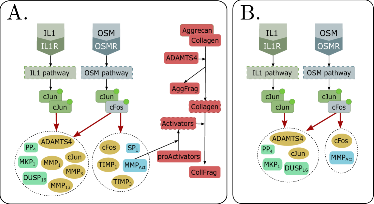
Figure 1: (A) Adaptation of the three molecular pathways from Proctor et al. (2014). (B) Reduced model obtained while preserving the phosphorylated forms of cJun and cFos. Dotted boxes represent abstractions of groups of biochemical species which are not fully shown here to reduce clutter.

This section discusses a pattern of modular decomposition similar to Section 4.1 in the main text, on a model of cartilage breakdown pathway from (Proctor et al., 2014), illustrated in Fig. 1(A). The model is available in the BioModels repository as BIOMD0000000504. The system comprises three modules: an Interleukin-1 (IL1) signaling pathway, an OSM signaling pathway, and a circuit of activation of proMMPs that concludes with the degradation of Aggrecan and Collagen.

In the first module, IL1 binds its receptor (ISMR) to start a cascade of phosphorylation events (not shown) that activates cJun. After dimerization, cJun upregulates collagenases MMP_{1,3,13} and phosphatases MKP1, PP 44 and DUSP16. In the second module, OSM binds to the receptor OSMR; the pathway concludes with the phosphorylation of cFos. The active cFos can reversibly bind to phosphorylated cJun in a complex cJun-cFos which acts as transcription factor and upregulates the transcription factor SP 1, TIMPs_{1,3}, cFos, cJun, a generic MMP_Activator and all the upregulated components from IL 1 module. In the third module, the Aggrecan-Collagen complex separates due to the interaction with ADAMTS 4, and the units of Aggrecan in the complex transform into fragments (AggFrag). The units of Collagen interact with several Activators (collagenases such as MMP_{1,3,13} or MMP_Act) that destroy the protein structure, producing collagen fragments (CollFrag).

The original model consists of 74 variables. By preserving the phosphorylated molecules of cFos and cJun, which are some of the species of interest in the study by Proctor et al. (2014), CLUE removes the pathway for the decomposition of the Aggrecan-Collagen complex, together with the mRNA variants of MMP_{1,3,13}, TIMP_{1,3}, and SP1. The reduced model with 43 variables can be interpreted as the network in Fig. 1 (B). Again, CLUE simplifies branches of the pathway that do not affect the dynamics of the observables. The reduction by forward equivalence, instead, collapses only the variables corresponding to the species Aggrecan, AggFrag, Collagen, and CollFrag, providing a model with 71 variables. Differently from the previous example, this block collapses end species (AggFrag and CollFrag) together with an input species (Aggrecan) which is assumed to have no dynamics (i.e., zero derivative), as well as a species (Collagen) that undergoes degradation.

V Comparison of Algorithm 2 and Algorithm 3

As mentioned in the main text, Algorithm 2 is typically faster for simpler cases, while the performance of Algorithm 3 is more robust. The ratios of the runtime of Algorithm 3 and the runtime of Algorithm 2 for an extended set of benchmarks are collected in Table 1 below. The value $<0.01$ refers to the fact that Algorithm 2 has been running for 100 times more than the runtime of Algorithm 3 but did not produce any result and has been stopped. The benchmarks are available in the repository https://github.com/pogudingleb/CLUE/tree/master/examples. For three of the models, we had several sets of observables, the indexes of the sets (as listed in the repository) are given in the parenthesis.

From the table, one can see that Algorithm 2 is faster than Algorithm 3 by about a factor of $6$ for the majority of given examples. Typically, this happens if the dimension of the reduced model is relatively small or the form of reduction is relatively simple. On the other hand, in the cases in which Algorithm 2 encounters very long integers during the computation (like (Barua et al., 2009) and (Faeder et al., 2003) models), it is likely to get stuck while Algorithm 3 terminates in reasonable yielding to more than 100-fold speed up.

Model	time(Alg. 3) / time(Alg. 2)
Li et al. (2006)	$2.5$
Proctor et al. (2014) (1)	$3.0$
Proctor et al. (2014) (2)	$4.0$
Proctor et al. (2014) (3)	$3.2$
Proctor et al. (2014) (4)	$4.0$
Borisov et al. (2008)	$6.0$
Sneddon et al. (2011), $m=2$	$5.0$
Sneddon et al. (2011), $m=3$	$5.0$
Sneddon et al. (2011), $m=4$	$6.0$
Sneddon et al. (2011), $m=5$	$6.7$
Sneddon et al. (2011), $m=6$	$6.9$
Sneddon et al. (2011), $m=7$	$6.7$
Sneddon et al. (2011), $m=8$	$6.6$
Barua et al. (2009) (1)	$\mathbf{<0.01}$
Barua et al. (2009) (1)	$\mathbf{<0.01}$
Pepke et al. (2010)	$4.0$
Faeder et al. (2003) (1)	$5.2$
Faeder et al. (2003) (2)	$\mathbf{<0.01}$
Faeder et al. (2003) (3)	$5.8$
Faeder et al. (2003) (4)	$5.6$
Faeder et al. (2003) (5)	$6.6$

Table 1: The ratio of the runtimes of Algorithm 3 and Algorithm 2 for an extended set of benchmarks
The numbers in parenthesis after a reference refer to the index of the chosen set of observables.

In our implementation, these algorithms are combined to benefit from their strengths as follows. We first run Algorithm 2, and if the algorithm encounters very long rational numbers (we use $10000$ digits as the threshold), then we stop it and run Algorithm 3 instead. In the most frequent case of not so long rational numbers, the runtime is the same as that of Algorithm 2. In the cases in which using Algorithm 3 is preferable, first trying Algorithm 2 in our implementation adds only a small overhead (less than 10%) compared to running Algorithm 3 by itself.

References

- Barua et al. [2009] D. Barua, J. R. Faeder, and J. M. Haugh. A bipolar clamp mechanism for activation of jak-family protein tyrosine kinases. PLoS Comput. Biol., 5(4):e1000364, 04 2009. URL http://dx.doi.org/10.1371/journal.pcbi.1000364.
- Borisov et al. [2008] N. Borisov, A. Chistopolsky, J. Faeder, and B. Kholodenko. Domain-oriented reduction of rule-based network models. IET systems biology, 2(5):342–351, 2008. URL https://dx.doi.org/10.1049/iet-syb:20070081.
- Cardelli et al. [2017] L. Cardelli, M. Tribastone, M. Tschaikowski, and A. Vandin. Maximal aggregation of polynomial dynamical systems. PNAS, 114(38):10029–10034, 2017. URL https://doi.org/10.1073/pnas.1702697114.
- Faeder et al. [2003] J. R. Faeder, W. S. Hlavacek, I. Reischl, M. L. Blinov, H. Metzger, A. Redondo, C. Wofsy, and B. Goldstein. Investigation of early events in fcri-mediated signaling using a detailed mathematical model. The Journal of Immunology, 170(7):3769–3781, 2003. doi: 10.4049/jimmunol.170.7.3769. URL https://doi.org/10.4049/jimmunol.170.7.3769.
- Li and Rabitz [1989] G. Li and H. Rabitz. A general analysis of exact lumping in chemical kinetics. Chemical Engineering Science, 44(6):1413–1430, 1989. URL https://doi.org/10.1016/0009-2509(89)85014-6.
- Li and Rabitz [1991] G. Li and H. Rabitz. New approaches to determination of constrained lumping schemes for a reaction system in the whole composition space. Chemical Engineering Science, 46(1):95–111, 1991. URL https://doi.org/10.1016/0009-2509(91)80120-N.
- Li et al. [2006] J. Li, L. Wang, Y. Hashimoto, C. Tsao, T. Wood, J. Valdes, E. Zafiriou, and W. Bentley. A stochastic model of escherichia coli AI-2 quorum signal circuit reveals alternative synthesis pathways. Molecular systems biology, 2(1), 2006. URL https://dx.doi.org/10.1038/msb4100107.
- Pepke et al. [2010] S. Pepke, T. Kinzer-Ursem, S. Mihalas, and M. B. Kennedy. A dynamic model of interactions of ca2, calmodulin, and catalytic subunits of ca2/calmodulin-dependent protein kinase II. PLoS Computational Biology, 6(2):e1000675, 2010. URL https://doi.org/10.1371/journal.pcbi.1000675.
- Proctor et al. [2014] C. Proctor, C. Macdonald, J. Milner, A. Rowan, and T. Cawston. A computer simulation approach to assessing therapeutic intervention points for the prevention of cytokine-induced cartilage breakdown. Arthritis & rheumatology, 66(4):979–989, 2014. URL https://doi.org/10.1002/art.38297.
- Sneddon et al. [2011] M. Sneddon, J. Faeder, and T. Emonet. Efficient modeling, simulation and coarse-graining of biological complexity with NFsim. Nature methods, 8(2):177, 2011. URL https://doi.org/10.1038/nmeth.1546.
- Trefethen and Bau [1997] L. N. Trefethen and D. I. Bau. Numerical Linear Algebra. SIAM, 1997.
- von zur Garthen and Gerhard [2013] J. von zur Garthen and J. Gerhard. Modern Computer Algebra. Cambridge University Press, 2013.
- Wang [1981] P. Wang. A -adic algorithm for univariate partial fractions. In Proceedings of SYMSAC’81, pages 212–217, 1981. URL https://doi.org/10.1145/800206.806398.
- Wang et al. [1982] P. Wang, M. Guy, and J. Davenport. -adic reconstruction of rational numbers. SIGSAM Bulletin, 16(2):2–3, 1982. URL https://doi.org/10.1145/1089292.1089293.