An Abstraction-guided Approach to
Scalable and Rigorous Floating-Point Error Analysis

Abstract

Automated techniques for rigorous floating-point round-off error analysis are important in areas including formal verification of correctness and precision tuning. Existing tools and techniques, while providing tight bounds, fail to analyze expressions with more than a few hundred operators, thus unable to cover important practical problems. In this work, we present Satire, a new tool that sheds light on how scalability and bound-tightness can be attained through a combination of incremental analysis, abstraction, and judicious use of concrete and symbolic evaluation. Satire has handled problems exceeding 200K operators. We present Satire’s underlying error analysis approach, information-theoretic abstraction heuristics, and a wide range of case studies, with evaluation covering FFT, Lorenz system of equations, and various PDE stencil types. Our results demonstrate the tightness of Satire’s bounds, its acceptable runtime, and valuable insights provided.

1 Introduction

Floating-point arithmetic underlies many critical scientific and engineering applications. Round-off errors introduced during floating-point computations have resulted in egregious errors in applications ranging from statistical computing and econometric software [33, 2] to critical defense systems [39]. To guard against such errors, formal verification tools are essential, and a basic capability in such tools is the ability to rigorously estimate the round-off error generated by floating-point expressions for given input intervals. This capability is also important in designing rigorous mixed-precision tuning systems (e.g., [9]).

A number of tools for rigorous round-off analysis have been developed: Fluctuat [14], Gappa [13], PRECiSA [49], Real2Float [31], Rosa [12], FPTaylor [47], Numerors [26], and tools specialized for cyberphysical systems [36, 43] to name a few. Unfortunately, these tools cannot automatically handle floating-point expressions of thousands of operators that arise in even the simplest of practical situations including recurrence equation solving schemes and algorithms such as the Fast Fourier Transform (FFT) and parallel prefix sum. Today’s tools in this space can at best handle expressions with a few dozen operators. To tackle large sizes automatically, one must today employ abstract interpretation methods and/or theorem-proving methods [14, 36, 37, 5]. The use of non-rigorous approaches that employ concrete evaluation on a reasonable sampling of the input space [42, 21, 38, 28, 35] or Monte-Carlo-style approached [15, 44] is also popular. While such approaches are ultimately inevitable, formal verification is essential for critical tasks such as aircraft collision avoidance verification [19]. A higher degree of automation can greatly help with these verification tasks.

An analysis method’s ability to derive tight bounds is as important as its ability to handle large expressions graphs. Interval analysis provides an efficient and fast way to obtain error bounds; however, it inherently loses correlation between terms, resulting in quite pessimistic bounds. While affine analysis maintains correlations between error variables by keeping them formal (symbolic), it can also result in pessimistic bounds, especially for non-linear expressions such as $x/(x+1)$, where the non-linearity is introduced by division.

In this work, we introduce a scalable and rigorous approach for error analysis embedded in a new tool, namely, Satire (Scalable Abstraction-guided Technique for Incremental Rigorous analysis of round-off Errors). Satire supports scalable mixed-precision analysis and multi-output estimation of straight-line floating-point code. We demonstrate that Satire can perform error estimation for complex expression graphs involving thousands of operators, including FFTs, recurrence equations, and partial differential equation (PDE) solving.

The recently proposed method of rigorously computing symbolic Taylor forms and embodied in the FPTaylor tool [47] avoids problems associated with interval and affine methods. Moreover, as the table of results in [47] and [26] show, FPTaylor also produces some of the tightest bounds when compared to the tools in its class. However, FPTaylor cannot handle large expression graphs. For example, for the discretized one-dimensional heat flow (“1D-heat”) equation calculation using a stencil whose temporal application is unrolled over 10 time steps, about 442 expression nodes are generated. FPTaylor takes about 8 hours simply to generate the Taylor form expression, following which its global optimizer fails to handle this expression. In contrast, Satire handles the aforesaid 1D-heat problem in a few seconds, generating tight bounds. Satire also has handled expressions with over 200K operators drawn from realistic examples. In addition, Satire generates tighter error bounds than FPTaylor on most of FPTaylor’s examples. To give an early indication of Satire’s performance, Table 1 provides a sampling of examples (comprehensive evaluations in §2 and §6).

Benchmarks	# operators	Exec Time (secs)		Absolute Error		Empirical Max Abs Error
		Satire	FPTaylor	Satire	FPTaylor
jetEngine	35	1.969	0.84	2.88E-08	7.09E-08	1.57E-12
kepler2	43	0.402	0.52	3.20E-12	2.53E-12	3.49E-13
dqmom	35	0.206	0.63	9.66E-10	6.91E-05	3.27E-13
1D-heat-10steps	442	2.1	-	6.11E-15	NA	5.45E-16
FFT-1024pt	43K	180	-	7.80E-13	NA	6.18E-15
Lorenz-20steps	307	284	-	1.25E-14	NA	3.59E-15

The benchmarks Jetengine, Kepler, and DQMOM are some of the largest that have been handled by FPTaylor, but contain no more than a few dozen operators. The much larger benchmarks including FFT-1024pt (an FFT computation of 1K inputs), and Lorenz-20steps (a Lorenz system that captures the “butterfly effect”) are all representative of practically important examples. They far exceed the capability of all existing round-off error analysis tools. The last column of the table presents the empirically calculated (using shadow values) maximum absolute error over $10^{6}$ simulations for randomly selected data points from the input intervals. Lacking other means of easily obtaining tight rigorous bounds, these results provide a good indication of how close Satire’s bounds are.

Satire only analyzes for first-order error. To check whether we are lacking precision due to this, we ran FPTaylor on its own benchmarks with its second-order error analysis turned off, only finding that the resulting error values were still bit-identical. This shows that it can be very difficult to create examples where second-order error matters. In [29], the authors further emphasize this point by mentioning that they had to refine their second-order error analysis beyond the approach taken in FPTaylor.

Roadmap:

In §2, we explain Satire’s contributions at a high level; this helps better understand the remainder of the paper. In §2, we explain the essential background on floating-point arithmetic and the global optimization-based error analysis done in Satire.We also point out the key contributions made by Satire. In §3, we explain the incremental analysis adopted in Satire. §4 presents the formal details of Satire’s error analysis with heuristics for abstraction and for improving global optimization/canonicalization detailed in §5. §6 presents a comprehensive evaluation of Satire on many practical examples. §7 presents additional related work. §8 has our concluding remarks.

2 Background, Contributions

A binary floating-point number systems, $\mathbb{F}$, is a subset of real numbers representable in finite precision and expressed as tuple $(s,m,e,p)$ with $p=53$ and $24$ for double and single precision numbers, respectively, $s\in\{-1,1\}$ is the sign bit, $m$ the mantissa, and $e$ the exponent. We consider only normal numbers where $m\in[1,2)$. Any such number, $\tilde{x}\in\mathbb{F}$ has the value $s\cdot m\cdot 2^{e}$. If $x\in\mathbb{R}$, then $\tilde{x}$ denotes an element in $\mathbb{F}$ closest to $x$ obtained by applying the rounding operator($\circ$) to x. The IEEE 754 standard defines four rounding modes for elementary floating-point operations. Every real number $x$ lying in the range of $\mathbb{F}$ can be approximated by a member $\tilde{x}\in\mathbb{F}$ with a relative error no larger than the unit round-off $\bf{u}=\dfrac{1}{2}2^{1-p}$. Here, $2^{1-p}$ represents the unit of least precision (ulp) for the exponent value of 1. Thus, to relate the quantities $\tilde{x}$ and $x$ over the rounding operator, if $x\in\mathbb{R}$ lies in the range of $\mathbb{F}$, then $\tilde{x}=\circ(x)=x(1+\delta),\quad|\delta|\leq\boldsymbol{u}.$

Given two exactly represented floating-point numbers, $\tilde{x}$ and $\tilde{y}$, arithmetic operators $\diamond\in\{+,-,\cdot,/\}$ have the following guarantees:

$$\begin{split}\circ(\tilde{x}\diamond\tilde{y})&=(\tilde{x}\diamond\tilde{y})(1+\delta),\quad|\delta|\leq\boldsymbol{u}\\ &=(\tilde{x}\diamond\tilde{y})+(\tilde{x}\diamond\tilde{y})\delta=\{\hbox{real value}\}+\{\hbox{ round-off error }\}\end{split}$$ (1)

Thus, the rounded result involves an interval centered around the real exact value. The width of this interval is determined by the amount of round-off error accumulated. Besides the elementary operators, Satire supports other complex mathematical operations such as transcendentals. In such cases, the bound on the $\delta$ terms changes as a multiple of $\bf{u}$. We keep a default configurable value for each operator, allowing the user to obtain customized error bounds for the specific math library being used.

Affine arithmetic [48] is often employed to keep errors correlated. A real number $\hat{x}$ is represented in affine form as $\hat{x}=x_{0}+\sum_{i=1}^{n}x_{i}\epsilon_{i}$, where $x_{0}$ denotes the central value and the $x_{i}$’s are finite floating-point numbers representing noise coefficients associated with the corresponding noise variables, $\epsilon_{i}$’s. The $\epsilon_{i}$ are formal variables whose value lies in $[-1,1]$ but are unknown until assigned. This representation allows converging paths to cancel out error terms and improve tightness. For example $(x-x)$ in affine analysis will yield 0 because the noise variables can cancel each other out. Unlike affine analysis, interval analysis keeps widening the intervals. Satire’s approach can be viewed as “symbolic affine” (much like FPTaylor) in that the noise coefficients, $x_{i}$, are symbolic, as further clarified in §2.

We use the following notations and conventions in the upcoming sections. We assume that an expression ${\cal E}$ defined over inputs ${\bf X}$ is being analyzed for the round-off error, given that each $x_{i}\in{\bf X}$ is instantiated with input interval $I_{i}\in{\bf I}$. Here, ${\cal E}$ is assumed to be represented as a DAG, and the process of analyzing ${\cal E}$ consists of somehow obtaining the error at each interior DAG node $i$, represented by ${\cal E}_{i}$, and then calculating how much this error contributes to the final error. Suppose ${\cal E}{rr}_{i}$ be the error generated by subexpression ${\cal E}_{i}$ (details in §4). We also use the notation $E_{i}$ and $E$ (respectively) to denote ${\cal E}_{i}$ and ${\cal E}$ that have been evaluated to ground values (fully evaluated after variable substitutions) by instantiating $x_{i}\in{\bf X}$ with intervals $I_{i}\in{\bf I}$. We now explain how Satire ensures scalability (Page 2) and tight bounds (Page 2).

Contributions Toward Scalability: Incremental Approach

Satire adopts an incremental approach while generating the error contributions of node ${\cal E}_{i}$ to the final output. In other words, we perform a breadth-first walk of the expression DAG of ${\cal E}$, enumerating subexpression nodes ${\cal E}_{i}$. At each ${\cal E}_{i}$, we perform first-order error analysis (see §4) of the total error generated at ${\cal E}_{i}$ to compute the error expression ${\cal E}{rr}_{i}$. We then multiply this error with the path strength of all the paths going from ${\cal E}_{i}$ to ${\cal E}$. Let there be $M$ such paths with path strengths $p_{1},p_{2},\ldots p_{M}$. In many examples such as 1D-heat, $M$ grows exponentially with the depth of ${\cal E}_{i}$ due to path reconvergence in expression DAGs.

In FPTaylor, the Symbolic Taylor Form ends up having the form $\Sigma_{j=1}^{M}\;(p_{j}\cdot{\cal E}{rr}_{i})$ which is huge for large $M$, as the error expression ${\cal E}{rr}_{i}$ is replicated $M$ times. This replication happens multiple times, explaining why it took 8 hours to generate its Symbolic Taylor Form for 1D-heat.

With Satire, we first compute ${\cal E}{rr}_{i}$ as explained in §4. We then compute ${\cal E}{rr}_{i}\cdot\Sigma_{j=1}^{M}\;p_{j}$, which is the product of the error with the effective path strength $\Sigma_{j=1}^{M}\;p_{j}$, taking all the paths from ${\cal E}_{i}$ to $E$ into account. This is significantly smaller in that it does not replicate ${\cal E}{rr}_{i}$ a very large number of times. This explains why Satire finished on 1D-heat in a few seconds even without using abstractions. Generating such factored forms also aids SimEngine [46] (detailed below under “canonicalizations”).

Automated Introduction of Abstractions: During a bottom-up (forward) pass to build ${\cal E}$, Satire performs symbolic execution to build the symbolic expression for ${\cal E}_{i}$. While doing so, Satire uses a heuristic to decide whether or not to automatically create an abstraction for ${\cal E}_{i}$.

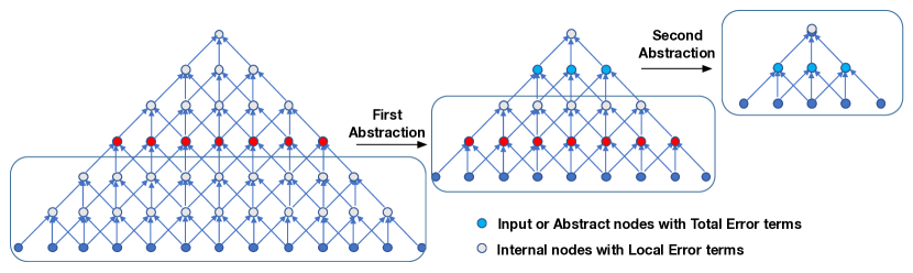
Figure 1: Incremental error analysis using gradual abstraction

Figure 1 illustrates this incremental abstraction scheme. We employ a cost metric based on information-theory [45] to obtain a set of cut-points in the abstract syntax tree (AST). Each of these cut-points serve as the ${\cal E}_{i}$ for which abstractions are created. The selected cut-points then become free variables, carrying concrete error interval bounds (explained below) for the rest of the error analysis. In Figure 1, we introduce our first abstraction at height 2 for a stencil-type computation.

Clearly there is a risk of losing variable correlations in the process. In §5, we point out that with well-chosen heuristics, this risk can be minimized, providing still tight error estimates. These abstractions are key to Satire’s performance on larger examples, and can be viewed as an appropriate tradeoff between scalability and bound tightness. By performing abstractions, the error analysis at each of the abstracted nodes ${\cal E}_{i}$ is a much more manageable process and finishes quickly. Secondly, we incrementally compute the error bounds of ${\cal E}_{i}$ with respect to the variables ${\bf X}_{i}$ mentioned in it using a global optimization call that refers to the appropriate intervals ${\bf I}_{i}$. This is a much smaller optimization query that finishes fast. The resulting error expression is a concrete value interval that is propagated upstream for further error analysis. In other words, during Satire’s analysis, a mixture of symbolic and concrete error intervals are propagated across the expression DAG. This dramatically reduces overall error analysis complexity.

Contributions Toward Tight Bounds:

Expression Canonicalization: A central step that is involved at every stage in Satire’s operation is this: given an expression ${\cal E}$ and the intervals in which the variables in ${\cal E}$ lie, compute the tightest interval bound for ${\cal E}$. Consider computing this for a simple expression such as $x\cdot x\cdot x$ using an interval library such as Gaol where $x\in[-1,5]$. Gaol would perform two successive interval multiplications, resulting in $[-25,125]$. To allow users to obtain better bounds, Gaol provide a special interface function $pow$ using which the above call can be written as $pow(x,3)$. Intuitively the use of functions such as $pow(x,3)$ conveys the information that the same $x$ instance is being acted upon, allowing Gaol to obtain $[-1,125]$. Unfortunately, there are only a limited number of interface functions such as $pow$, and therefore, in general, an external canonicalizer must be used to reduce the number of distinct occurrences of variables in an expression. SimEngine’s “expand” strategy allows us to achieve this effect, which then allows the back-end optimizer Gelpia (that uses the interval branch-and-bound algorithm) to converge to tight bounds much more quickly. For the DQMOM example in Table 1, this was the main reason why we improved upon FPTaylor’s result of 6.9e-05 to 9.6e-10 in Satire (§4).

Avoid Impeding Canonicalization: Not only must explicit canonicalization be performed wherever possible, we avoid taking steps that can block canonicalization. To be more specific, denote the sum of path strengths at expression site ${\cal E}_{i}$, i.e., $\Sigma_{j=1}^{M}\;p_{j}$, by ${\cal S}_{i}$. When we perform a depth-oriented traversal of the expression DAG, let us imagine generating expressions ${\cal E}_{1},\ldots,{\cal E}_{K}$ (where the ${\cal E}_{i}$ are the subexpressions of ${\cal E}$) with corresponding errors ${\cal E}{rr}_{1},\ldots,{\cal E}{rr}_{K}$. The final error at the output of ${\cal E}$ is ${\cal E}{rr}=\Pi_{i=1}^{K}\;{\cal S}_{i}\cdot{\cal E}{rr}_{i}$. Let the final concrete error at the output of ${\cal E}$ be $Err$. There are two ways to arrive at $Err$: (1) As a concretization of $\Pi_{i=1}^{K}\;abs({\cal S}_{i}\cdot{\cal E}{rr}_{i})$; or (2) As a concretization of $\Pi_{i=1}^{K}\;abs({\cal S}_{i})\cdot abs({\cal E}{rr}_{i})$. While both these are real-number equivalent, the latter expression blocks canonicalizations from occurring within SimEngine. All our results jumped from being worse than FPTaylor’s to being better than FPTaylor’s when we adopted the former form (the jump from Satire (UnOpt) to Satire in Table 1).

3 Illustrative Example

In Satire, a floating-point straight line program is parsed into an abstract syntax tree (AST) where each node of the AST is an operator (e.g., $\{+,-,\cdot,/\}$ or others such as $exp$ and transcendentals). Figure 2 shows the AST for the expression $S=(x\cdot(x+y)+z)\cdot 3.5$. Here, $x$, $y$, and $z$ are the input variables with intervals $I(x)$, $I(y)$, and $I(z)$, respectively. In  [12, 24], the authors introduce the decomposition of errors into generated round-off errors and propagation of incoming errors. We use ${\cal E}^{lr}$ to denote the local error term associated with a node. The total error term for a node, denoted as ${\cal E}^{tr}$, is then the additive composition of ${\cal E}^{lr}$ and the propagation of the incoming error, ${\cal E}^{prop}$. We annotate each interior node in Figure 2 with a pair consisting of its symbolic function expression and a symbolic local error term. An abstracted node is treating as an additional input, wherein we take the convention of using the variable name as the symbolic expression for an input node, and instead of the local error, we employ the total error term (as detailed below these input nodes are not modeled).

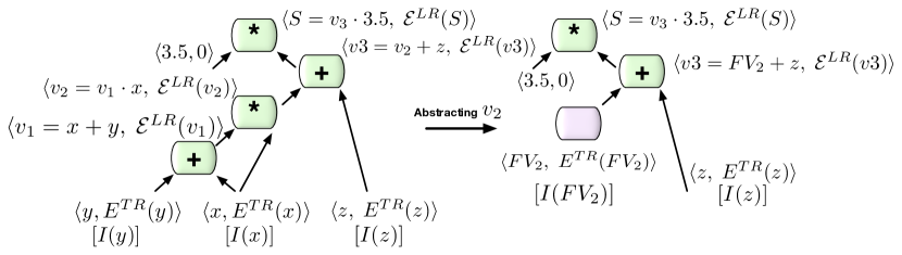
Figure 2: AST for $S=(x\cdot(x+y)+z)\cdot 3.5$, and the rebuilt AST with $v_{2}$ abstracted. The equations analyzed are $v_{1}=x+y;\;\;v_{2}=v_{1}\cdot x;\;\;v_{3}=v_{2}+z;\;\;S=v_{3}\cdot 3.5$.

Consider node $v_{2}$ with associated symbolic expression $v_{1}\cdot x$. Its incoming error is a symbolic expression denoted by ${\cal E}^{lr}(v_{2})$. From Equation 1:

$$\begin{split}{\cal E}^{tr}(v_{2})={\cal E}^{lr}(v_{2})+{\cal E}^{prop}(v_{2})\ &={\cal E}^{lr}(v_{2})+\left(E^{tr}(x)\dfrac{\partial v_{2}}{\partial x}+{\cal E}^{tr}(v_{1})\dfrac{\partial v_{2}}{\partial v_{1}}\right)\\ &={\cal E}^{lr}(v_{2})+\left(E^{tr}(x)\cdot v_{1}+{\cal E}^{tr}(v_{1})\cdot x\right)\end{split}$$ (2)

The derivatives signify the sensitivity of $v_{2}$ w.r.t. their operands. Similarly,

$$\begin{split}{\cal E}^{tr}(v_{1})={\cal E}^{lr}(v_{1})+{\cal E}^{prop}(v_{1})&={\cal E}^{lr}(v_{1})+\left(E^{tr}(x)\dfrac{\partial v_{1}}{\partial x}+E^{tr}(y)\dfrac{\partial v_{1}}{\partial y}\right)\\ &={\cal E}^{lr}(v_{1})+\left(E^{tr}(x)\cdot 1+E^{tr}(y)\cdot 1\right)\end{split}$$ (3)

Plugging Equation$~{}\eqref{eq:v1-unroll}$ into Equation$~{}\eqref{eq:internal-node-error}$, we obtain the total error for $v_{2}$ in terms of the local errors and incoming errors on inputs:

$${\cal E}^{tr}(v_{2})={\cal E}^{lr}(v_{2})+(2x+y)E^{lr}(x)+x\cdot{\cal E}^{lr}(v_{1})+x\cdot E^{tr}(y)$$ (4)

The extent to which the error accumulated at $v_{2}$ impacts the output at $S$ depends on the sensitivity of $S$ to changes in $v_{2}$, that is, $\dfrac{\partial S}{\partial v_{2}}=\dfrac{\partial S}{\partial v_{3}}\dfrac{\partial v_{3}}{\partial v_{2}}=3.5$

Let ${\cal E}^{tr}(S|v_{2})$ denote the total error component at the output node, $S$, due to total error accumulated at $v_{2}$ (path-strength from $v_{2}$ to $S$); then:

$$\begin{split}{\cal E}^{tr}(S|v_{2})={\cal E}^{tr}(v_{2})\dfrac{\partial S}{\partial v_{2}}&=\left({\cal E}^{lr}(v_{2})+(2x+y)E^{lr}(x)+x\cdot{\cal E}^{lr}(v_{1})+x\cdot E^{tr}(y)\right)\cdot 3.5\\ &={\cal E}^{lr}(v_{2})\dfrac{\partial S}{\partial v_{2}}+E^{tr}(x)\dfrac{\partial S}{\partial x}+{\cal E}^{lr}(v_{1})\dfrac{\partial S}{\partial v_{1}}+E^{tr}(y)\dfrac{\partial S}{\partial y}\end{split}$$ (5)

Equation$~{}\eqref{eq:v2-total-error-expr}$ is the symbolic form of the error contribution from $v_{2}$ (and all its dependencies) to $S$. There are two approaches to obtain the bound on ${\cal E}^{tr}(S|v_{2})$:

1. Without abstraction, where we feed the optimizer with the fully symbolic expression of ${\cal E}^{tr}(S|v_{2})={\cal E}^{tr}(v_{2})\dfrac{\partial S}{\partial v_{2}}$. This formulation preserves all variable correlations (especially important for non-linear expressions) and is expected to obtain the tightest possible bounds. However, the resulting large expressions can often end up choking the global optimizer or excessively delay its convergence.

2. With abstraction of node $v_{2}$. First we obtain a function interval and the total error by solving for $v_{2}$ and $E^{tr}(v_{2})=\max(|{\cal E}^{tr}(v_{2})|)$ using a global optimizer. Now, $v_{2}$ can be abstracted as a free variable, $FV_{2}$, with an associated error term ($E^{tr}(FV_{2})=E^{tr}(v_{2})$) and an interval range as shown in RHS of figure 2. Then reconstruct ${\cal E}^{tr}(S|v_{2})=E^{tr}(v_{2})\dfrac{\partial S}{\partial v_{2}}$, and feed it to the global optimizer to obtain the concrete bound, $E^{tr}(S|v_{2})$. This reduces the the query sizes submitted to the optimizer.

Note in our example that abstracting node $v_{2}$ completely removed the dependency from $v_{1}$ and $x$, and, therefore, was a good choice for abstraction. However, consider the case of $v_{1}$ being abstracted. This would result in a loss of correlation between the reconvergent paths merging at $v_{2}$ for input $x$. This can result in looser error bounds, especially when error cancellations occur in the merging paths. Error cancellations are important to include in floating-point error analysis in order to obtain tight error bounds.

Also, to find the total error at $v_{2}$, we unrolled its operand’s error term, $E^{tr}(v_{1})$ as well. Instead, if we only tracked the local error term at each node and scaled them by their respective propagation factors (“path strengths”) to the output, we end up with the same expression as in the last part of equation$~{}\eqref{eq:v2-total-error-expr}$. In contrast to existing tools, Satire identifies this balance in finding designated cut-points where we can solve internal nodes for total error terms and abstract them, removing their child dependencies. This process is repeated until the AST reaches a size that is easily managed using direct solve (unrolling all to local error terms; see Figure 1):

4 Error Analysis

We now define the first-order error analysis underlying Satire ending with a soundness claim. Let the expression to be analyzed be presented as a straight-line program with one output being $s$ (other outputs are similarly treated):

$$s=({\bf x},s_{1},s_{2},\dots,s_{n})$$

Here $\bf{x}$ is the set of $m$ incoming inputs, $\{x_{1},x_{2},\dots,x_{m}\}$ with $m$ incoming error quantities, $\{e_{x_{1}},e_{x_{2}},\dots,e_{x_{m}}\}$. Here, we think of $s_{i}$ as having been computed at the $i$th step of the overall computation, where $f_{i}$ are the operators supported:

$$s_{i}=f_{i}({\bf x},s_{1},s_{2},\dots,s_{i-1})$$ (6)

Equation$~{}\eqref{eq:iseq}$ represents the causality of the execution order, that is, the operator $f_{i}$ being computed in the $i$th step can involve as its inputs the primary inputs, ${\bf x}$, and any of the intermediary computed results leading upto the $i$th stage. When such a computation is performed in finite precision, the operators $f_{i}$ are replaced by their floating-point counterparts denoted as $\tilde{f_{i}}$. In addition to generating a round-off error component at the operator site, $\tilde{f_{i}}$ also propagates the incoming errors through each operand. Thus, the $i$th step of the algorithm with floating point operators is specified as

$$\begin{split}\tilde{s_{i}}&=\tilde{f_{i}}(\tilde{{\bf x}},\tilde{s_{1}},\tilde{s_{2}},\dots,\tilde{s_{i-1}})\\ &=\tilde{f_{i}}(x_{1}+e_{x_{1}},\dots,x_{m}+e_{x_{m}},s_{1}+e_{s_{1}},s_{2}+e_{s_{2}},\dots,s_{i-1}+e_{s_{i-1}})\\ \end{split}$$ (7)

Here, every $e_{s_{j}}$ denotes the total error flowing in to the operator site due to the accumulation at $s_{j}$, that is $e_{s_{j}}={\cal E}^{tr}(s_{j})$. Each $\tilde{f_{i}}$ generates as round-off error according to the equation$~{}\eqref{eq:opbound}$ , thus relating the real and floating point evaluation as

$$\begin{split}\tilde{s_{i}}=f_{i}(x_{1}+e_{x_{1}},\dots,x_{m}+e_{x_{m}},s_{1}+e_{s_{1}},\dots,s_{i-1}+e_{s_{i-1}})(1+\delta_{i});\quad|\delta_{i}|\leq\bf{u}\end{split}$$ (8)

If $s_{n}$ is the final step of the algorithm, then one could write its corresponding floating point $\tilde{s_{n}}$ as

$$\tilde{s_{n}}=f_{n}(x_{1}+e_{x_{1}},\dots,x_{m}+e_{x_{m}},s_{1}+e_{s_{1}},\dots,s_{i-1}+e_{s_{n-1}})(1+\delta_{n});\quad|\delta_{n}|\leq\bf{u}$$

A Taylor series expansion of the $f_{n}$ term on the rhs leads to the following

$$\begin{split}\tilde{s_{n}}&=f_{n}(x_{1}+e_{x_{1}},\dots,x_{m}+e_{x_{m}},s_{1}+e_{s_{1}},\dots,s_{i-1}+e_{s_{n-1}})(1+\delta_{n});\quad|\delta_{n}|\leq\bf{u}\\ &=\bigg{(}f_{n}({\bf x},s_{1},\dots,s_{n-1})+\sum_{j=1}^{n-1}\dfrac{\partial s_{n}}{\partial s_{j}}e_{s_{j}}+\sum_{j=1}^{m}\dfrac{\partial s_{n}}{\partial x_{j}}e_{x_{j}}\bigg{)}(1+\delta_{n})+O({\bf u}^{2})\\ &=f_{n}({\bf x},s_{1},\dots,s_{n-1})+f_{n}({\bf x},s_{1},\dots,s_{n-1})\delta_{n}+\sum_{j=1}^{n-1}\dfrac{\partial s_{n}}{\partial s_{j}}e_{s_{j}}+\sum_{j=1}^{m}\dfrac{\partial s_{n}}{\partial x_{j}}e_{x_{j}}+O({\bf u}^{2})\\ &=s_{n}+s_{n}\delta_{n}+\sum_{j=1}^{n-1}\dfrac{\partial s_{n}}{\partial s_{j}}e_{s_{j}}+\sum_{j=1}^{m}\dfrac{\partial s_{n}}{\partial x_{j}}e_{x_{j}}+O({\bf u}^{2})\\ \end{split}$$ (9)

Satire’s goal is to bound the absolute error on the output $s_{n}$, that is $e_{s_{n}}={\cal E}^{tr}(s_{n})=|s_{n}-\tilde{s_{n}}|$. The term $s_{n}\delta_{n}$ is the round-off error generator at the $f_{n}$ operator site representing the local error term, ${\cal E}^{lr}(s_{n})$. Thus the bound on the absolute error can be evaluated as

$$\begin{split}E^{tr}(s_{n})&\leq\max(|{\cal E}^{tr}(s_{n})|)\\ &\leq\max\bigg{(}|s_{n}\delta_{n}|+|\sum_{j=1}^{n-1}\dfrac{\partial s_{n}}{\partial s_{j}}e_{s_{j}}|+|\sum_{j=1}^{m}\dfrac{\partial s_{n}}{\partial x_{j}}e_{x_{j}}|\bigg{)}+O({\bf u}^{2})\\ &\leq\max\bigg{(}|{\cal E}^{lr}(s_{n})|+|\sum_{j=1}^{n-1}\dfrac{\partial s_{n}}{\partial s_{j}}{\cal E}^{tr}(s_{j})|+|\sum_{j=1}^{m}\dfrac{\partial s_{n}}{\partial x_{j}}{\cal E}^{tr}(x_{j})|\bigg{)}+O({\bf u}^{2})\\ \end{split}$$ (10)

Equation$~{}\eqref{eq:total-final-form}$ makes three necessary distinctions as follows.

$\bullet$ The second order error terms contain $\bf{u}^{2}$ which is an extremely small quantity and becomes relevant to precision only when $n{\bf u}\approx 1$. Given that ${\bf u}=2^{-53}$, $n$ must approach $2^{53}$. We perform abstractions well before reaching this point.

$\bullet$ Error expressions such as ${\cal E}^{lr}$ and ${\cal E}^{tr}$ can coexits in two forms in Satire: (1) as a symbolic expression, and (2) as a numeric interval. Ultimately, when we do the abstractions or solve for the final output, the expressions are maximized to obtain the maximum error bound.

$\bullet$ While the right-hand side of Equation (10) involves additional total error terms, these can be further unrolled to obtain direct dependencies to the local error terms down the hierarchy and/or inputs and abstracted nodes.

As mentioned in §2 (and detailed now), Satire follows an incremental and decoupled strategy toward error analysis:

• A forward pass that assigns a local symbolic error term at each operator site, ${\cal E}^{lr}$.

• A backward pass that uses symbolic algorithmic differentiation to derive the propagation factors (path strengths or derivatives) from each operator site to the output nodes.

• Incremental abstractions of nodes as detailed in §5.

Due to the use of abstractions, expressions such as ${\cal E}^{tr}(s_{n})$ are comprised of both symbolic (“${\cal E}$”) and ground (“$E$”) representations. More specifically, suppose $\alpha$ denotes the set of nodes that have been abstracted to numeric (ground) error bounds, and $\beta=n-\alpha$ are the remaining nodes that are preserved symbolically. Equation (10) can be viewed as a combination of both ilks, as in:

$$\begin{split}E^{tr}(s_{n})&\leq\max(|\mathcal{E}^{lr}(s_{n})|+|\underset{s_{j}\in\beta}{\sum}\dfrac{\partial s_{n}}{\partial s_{j}}\mathcal{E}^{tr}(s_{j})|+|\underset{s_{j}\in\alpha}{\sum}\dfrac{\partial s_{n}}{\partial s_{j}}{E}^{tr}(s_{i})|+\sum_{j=1}^{m}|\dfrac{\partial s_{n}}{\partial x_{j}}{E}^{tr}(x_{j})|)\end{split}$$ (11)

Global optimizers are capable of entertaining such mixed “concolic” expressions.

Soundness: Satire’s error bounds are conservative:

This claim is easily proved based on the following observations. Satire’s error analysis is decoupled into (1) computing the local error symbolically, and (2) multiplying it with the sum of all path strengths, again symbolically. Computation of the local error is based on symbolic execution to which the accepted error model [22] in Equation 1 is applied. The method of adding the generated errors and propagating the errors is justified to be sound in [12, 24] (also the beginning of §3). Computing the path strengths using reverse-mode symbolic differentiation is again known to be sound [4]. Satire implements its own symbolic automatic differentiation. Last but not least, the abstractions introduced in Satire are also conservative in that new free variables are introduced in lieu of existing expression subgraphs. These free variables do not have any correlations with the other inputs. Their ground value intervals are also (recursively) computed using the same error analysis, and by induction (since these are subexpressions) their soundness follows.

5 Heuristics for Abstraction, Global Optimization

Heuristics for Abstraction:

Heuristics that trigger abstraction are based on: (1) relative depth (RD), measuring how close the node is to the output (the closer it is, the less the path strength to the output); (2) a cost function $\phi(opCount)$, measuring the size of the symbolic expression and the number of free variables in it (these require increased optimizer-time); and (3) fanout ($fanout$) from each operator site: large fanouts are indicative of a larger dependency footprint. While abstracting at such sites can hurt error cancellation due to path correlations, it helps handle heavily interconnected networks such as stencil-type applications or neural networks. The depth heuristics are inspired by Shannon’s information theory [45]. If $D$ is the total AST depth and $d_{i}$ is the depth of the $i$th node, its relative depth and the overall cost function is given by:

$$\begin{split}\hbox{depth info}(i)&=-\dfrac{d_{i}}{D}\log_{2}(\dfrac{d_{i}}{D})\\ \hbox{cost info}(i)&=\hbox{depth info}(i)\times(\#opCount(i))\times(\#fanout(i))\end{split}$$ (12)

Additional knobs include: (1) a fixed depth at which an abstraction is forced (ignoring the cost function); (2) a [minDepth, maxDepth] window within which Satire iteratively performs the abstraction and rebuilds ASTs. In case the depth of the rebuilt AST is below the specified minDepth, Satire computes the remaining expression directly (“direct-solve” in Figure 1).

Heuristics to Improve Global Optimization, Canonicalization:

Satire uses Gelpia [18] as the backend global optimizer. It implements an interval branch-and-bound algorithm (IBBA [1]) to obtain a tight interval containing the optima when solving for the error expressions. Essentially, when solving for an $n-variable$ expression, it searches an $n$-dimensional box of intervals defined on the inputs. IBBA produces queries by repeatedly dividing this $n$-dimensional box into smaller box (interval) queries, where each query comprises of the symbolic expression and the subdivided interval box. These queries are fed to an interval library (Gaol) that produces an output bound for that interval. The final output is the best fit $n$-dimensional box that produces the tightest error bound within a given tolerance and a limit on iterations to constrain the search algorithm.

Note that the optimizer works on real-valued expressions and must obtain a bound that contains the optimum. As pointed out in §2, Gaol can automatically canonicalize simple expressions such as $x\cdot x\cdot x$. However, as expressions become more complex with non-linear terms and multiple variables, the interval subdivision process gets further bottlenecked, producing loose intervals. Take, for example, the ‘direct quadrature moments method’ (DQMOM) benchmark captured in Equation$~{}\eqref{eq:dqmom}$, where $m_{i}\in[-1.0,1.0]$ and each of $w_{i}$ and $a_{i}$ belongs to $[0.00001,1.0]$:

$$\begin{split}r=&(0.0+((((w_{2}*(0.0-m_{2}))*(-3.0*((1.0*(a_{2}/w_{2}))*(a_{2}/w_{2}))))*1.0)\\ +&((((w_{1}*(0.0-m_{1}))*(-3.0*((1.0*(a_{1}/w_{1}))*(a_{1}/w_{1}))))*1.0)\\ +&((((w_{0}*(0.0-m_{0}))*(-3.0*((1.0*(a_{0}/w_{0}))*(a_{0}/w_{0}))))*1.0)+0.0))))\end{split}$$ (13)

When fed to Gelpia, the unsimplified expression for $r$ in DQMOM generates the interval [-9.0E+10, 9.0E+10]. However, the canonicalized expression (automatically done by SimEnginefor us), is

$$r=3.0*(a_{0}^{2})*m_{0}/w_{0}+3.0*(a_{1}^{2})*m_{1}/w_{1}+3.0*(a_{2}^{2})*m_{2}/w_{2}$$

and this reduces the occurrence of $w_{i}$ and $a_{i}$ instances. This yields an interval bound [-9.0E+05, 9.0E+05], which is 5 orders of magnitude tighter. As a result, the error bound on DQMOM is 6.9E-05 using FPTaylor and 9.6E-10 using Satire (Table 1). These canonicalizations plus steps to prevent canonicalization blocking (§2) are largely responsible for Satire’s superior overall bounds.

6 Evaluation

We first evaluate Satire on FPTaylor’s benchmarks (also provided at [16]), which includes a wide range of examples such as polynomials approximations and non-linear expressions, all of which consist of a few dozen operators. We then study Satire on a set of fresh benchmarks comprised of much larger expressions going up to nearly 200k operators (obtained by unrolling loops from specific implementations of these computations). One important example studied is FFT by separating the complex evaluation into real and imaginary datapaths (e.g., as done by researchers who implement FFT circuits [27]). We also study the Lorenz equation system, followed by a study of relative-error profiles exhibited by FDTD.

Experimental Setup:

Satire is compatible with Python3, and its symbolic engine is based on SimEngine [46] (related to SymPy). All benchmarks were executed with Python3.8.0 version on a dual 14-core Intel Xeon CPU E5-2680v4 2.60GHz CPUs system (total 28 processor cores) with 128GB of RAM. To arrive at an objective comparison, the core analysis algorithms were measured without any multicore parallelism (both for FPTaylor and Satire). The Gelpia solver does employ internal multithreading: we did not alter it in any way when we used either FPTaylor or Satire. All FPTaylor benchmarks used their specified data types. Larger benchmarks we introduced use double floating-point type. High-precision shadow value calculations were performed using GCC’s quadmath.

6.1 Comparative Study

Benchmarks	Execution Time(seconds)		Absolute Error			Num OPs
	Satire	FPTaylor	Satire	FPTaylor	Satire (UnOpt)
exp1x	0.083	0.60	6.19E-14	2.04E-13	6.19E-14	5
exp1x_32	0.087	0.42	9.71E-06*	0.00010	9.71E-06	5
carbonGas	0.084	0.74	2.07E-08	3.07E-08	9.71E-06	21
x_by_xy	0.068	0.42	1.19E-07	8.31E-07	9.71E-06	4
verhulst	0.066	0.47	4.27E-16	3.79E-16	4.47E-16	10
turbine3	0.154	0.49	3.58E-14	3.48E-14	4.10E-14	23
turbine2	0.102	0.49	6.32E-14	7.36E-14	7.39E-14	19
turbine1	0.097	0.50	4.89E-14	5.29E-14	5.60E-14	24
triangle	0.785	0.72	7.05E-14	4.06E-14	7.08E-14	14
test05_nonlin1_test2	0.063	0.40	1.11E-16	1.11E-16	1.38E-16	4
test05_nonlin1_r4	0.068	0.41	1.11E-06	2.78E-06	1.94E-06	6
test02_sum8	0.080	0.41	7.77E-15	7.11E-15	7.77E-15	15
test01_sum3	0.125	0.40	1.13E-06	1.97E-06	1.13E-06	11
sum	0.079	0.40	3.44E-15	3.66E-15	1.13E-06	11
sqrt_add	0.072	0.42	1.17E-15	8.86E-15	5.22E-15	7
sqroot	0.074	0.46	8.82E-16	6.00E-16	8.82E-16	25
sphere	0.069	0.42	8.88E-15	1.03E-14	8.88E-15	9
sine	0.122	0.50	7.36E-16	6.21E-16	7.36E-16	16
sineOrder3	0.065	0.44	1.09E-15	9.56E-16	1.09E-15	12
sec4_example	0.085	0.43	9.96E-10	1.83E-09	1.30E-09	8
rigidBody2	0.084	0.43	3.97E-11	3.61E-11	3.97E-11	17
predatorPrey	0.068	0.48	1.73E-16	1.74E-16	1.75E-16	12
nonlin2	0.081	0.43	9.96E-10	1.83E-09	1.30E-09	8
nonlin1	0.072	0.44	1.14E-13*	4.37E-11	2.92E-11	4
logexp	0.062	0.41	3.33E-13	8.90E-13	4.98E-13	5
jetEngine	1.969	0.84	2.88E-08	7.09E-08	2.88E-08	35
intro_example	0.069	0.40	1.14E-13*	4.37E-11	2.92E-11	4
i4	0.073	0.41	3.53E-07*	8.91E-06	3.53E-07	5
hypot32	0.066	0.40	8.43E-06*	0.00052	8.43E-06	6
himmilbeau	0.090	0.45	9.86E-13	1.00E-12	9.86E-13	13
exp1x_log	0.094	0.43	2.39E-12	1.38E-12	3.09E-12	6
bspline3	0.139	0.41	7.40E-17	7.86E-17	7.40E-17	7
delta4	0.119	0.45	1.26E-13	1.21E-13	1.26E-13	25
delta	0.416	0.53	3.30E-12	2.41E-12	3.30E-12	45
doppler1	0.158	0.58	1.49E-12	4.06E-13	1.71E-12	16
doppler2	0.164	0.59	2.98E-10	1.03E-12*	3.55E-10	16
doppler3	0.161	0.57	2.70E-13	1.60E-13	3.09E-13	16
hypot	0.068	0.41	3.37E-13	9.72E-13	6.53E-13	6
kepler0	0.094	0.43	1.10E-13	1.09E-13	1.10E-13	22
kepler1	0.168	0.46	7.07E-13	4.90E-13	7.07E-13	29
kepler2	0.402	0.52	3.20E-12	2.53E-12	3.20E-12	43
rigidBody1	0.076	0.41	3.80E-13	2.95E-13	3.80E-13	12
test04_dqmom9	0.206	0.63	9.66E-10*	6.91E-05	2.99E-05	35
test06_sums4_sum1	0.320	0.40	2.38E-07	6.26E-07	2.38E-07	7
test06_sums4_sum2	0.082	0.40	2.38E-07	6.26E-07	2.38E-07	7

Table 1: Comparison of Results (bold-face highlights better results, and * highlights a difference of more than an order of magnitude)

Table  1 presents the comparative results for Satire and FPTaylor. Comparison is presented for both the total execution times and the absolute error bounds over a suite of 47 benchmarks exported from FPTaylor’s suite. We observe that while Satire excels in its ability to handle large and complex expressions, even for smaller benchmarks it obtains comparable and, in many cases, tighter bounds than today’s state-of-the-art error analysis tools. In most cases, Satire and FPTaylor generated error bounds within the same orders of magnitude. Satire obtains even slightly tighter bounds in over 50% of these benchmarks while providing an average 4.5 times speed-up in execution time. Using $10^{6}$ random simulations on the input interval ranges we empirically verify Satire’s bound’s with respect to a high-precision shadow value evaluation of these benchmarks.

Furthermore, applying simplification procedures on FPTaylor’s generated symbolic taylor forms, we show improvement in its generated bounds. By default, Satire optimizes the product of the propagation factor and error term, that is, the “absolute” quantifiers are placed on the product terms. This helps to improve the expression simplification process. For many of the benchmarks in Table 1, Satire’s result without this optimization shows weaker results, but still within the same order of magnitude as FPTaylor.

6.2 Analysis of Larger Benchmarks

Table 2 summarizes the aforesaid large benchmarks where column ‘Full Solve’ indicates the bound obtained without any abstractions. Without abstractions, Satire fails to obtain answers for Lorenz, 2D-heat, and Gram-Schmidt (residual). For linear examples, the derivatives (propagation factors for the error terms) are always constant and, hence, do not impact the error expressions’s complexity. However, as expressions become non-linear (e.g., Lorenz), the propagation factors are not constants any more, leading to more complex error expressions. This is the primary reason why we can directly compute (“Full Solve”) a bound for FDTD with 192,000 operators without any abstractions—but for Lorenz, with merely 307 operators, we had to use abstractions. FPTaylor could not generate symbolic Taylor Forms for any of these expressions.

While abstractions help manage a large expression size, using abstractions frequently can impact the bounds. On a positive note, frequent abstraction implies smaller queries to the optimizer which helps to converge quicker exploring a smaller search space. Conversely, frequent abstraction will also lead to loss of correlation since we are replacing the symbolic expressions with concrete intervals. As a generic trend, while error bounds weaken if the frequency of abstractions is increased, they remain in the same order of magnitude. In examples such as FDTD, concretization of internal nodes during abstraction introduces large correlation losses. In the presence of cancellation terms (as in FDTD), preserving correlation is necessary because it enables symbolic error variables to cancel out. Abstractions inhibit this cancellation process and, hence, should be used judiciously in such examples.

Benchmarks	Num OPs	Absolute Error Bound					Best Execution Time
		Full Solve	Increasing frequency of Abstraction
			$\xrightarrow{\hskip 56.9055pt}$
FFT-1024pt	43k	7.89E-13	8.87E-13	9.57E-13	9.22E-13	9.70E-13	90s
Lorenz20(y)	307	NA	2.53E-14	2.61E-14	2.61E-14	3.17E-14	78s
Lorenz40(y)	607	NA	1.93E-13	2.69E-13	2.15E-13	2.16E-13	294s
Lorenz70(y)	1057	NA	1.88E-10	3.70E-07	1.07E-09	1.83E-09	1268s
Scan(1024pt ,[-1,1])	3060	1.88E-12	1.88E-12	1.88E-12	1.88E-12	1.88E-12	5s
fdtd(10)	6173	2.56E-14	7.56E-13	8.45E-13	5.43E-12	1.11E-10	17s
fdtd(64)	192k	7.45E-13	–	–	–	–	2.6 hrs
1D-heat(10)	442	6.10E-15	6.10E-15	6.10E-15	6.10E-15	6.10E-15	2.58s
1D-heat(32)	4226	1.95E-14	1.95E-14	1.95E-14	1.95E-14	1.95E-14	49s
2D-heat(32)	270k	NA	2.22E-14	2.22E-14	2.22E-14	2.22E-14	5 hrs
gSchmidt(r)	150	NA	1.14E-18	1.05E-18	1.05E-18	1.14E-18	12s
gSchmidt(Q)	150	1.22E-18	1.17E-18	1.13E-18	1.17E-18	1.13E-18	4s

Table 2: Larger Benchmarks with and without abstractions

To further motivate the importance of obtained rigorous bounds for large benchmark problems, we study FFT and Lorenz, both being critical components of high precision applications.

FFT:

Fast Fourier transform (FFT) is an optimized algorithm for discrete Fourier transform (DFT), which converts a finite sequence of sampled points of a function into a same length sequence of an equally numbered complex-valued frequency components. It has a vast number of applications in signal processing and fast multi-precision arithmetic for large polynomial and integer multiplications.

An $N$-point FFT involves $\log_{2}N$ stages, each stage having a familiar butterfly structure (see for example [8]). We are not aware of any tool supporting floating-point error analysis over complex domains. However, its application to fast math multi-precision libraries necessitates precise floating point error analysis and has been the subject of multiple analytical studies [41, 7, 40, 27]. These analysis methods focus on obtaining L2-norms in terms of root mean square (RMS) errors, or statistically profiled error bounds. Brisbarre et al. [8] followed up on the work from Percival’s [40, 7] to report the best L2-norm bound till date of $\approx 30.99ulps$. That is, if $z$ represents the discretized input samples, $Z$ is the exact result and $\hat{Z}$ is the computed result, then, $\dfrac{||Z-\hat{Z}||_{2}}{||Z||_{2}}\leq B\approx 30.99{\bf u}$

To extend this result to a bound on absolute error corresponding to the L-infinity norm, we utilize two well-known relations: (1) Between the L2 norms of the input and outputs of an $N$-point FFT, i.e., $||Z||_{2}\leq\sqrt{N}\cdot||z||_{2}$, and (2) a generic relation between the L-infinity norm and L2-norm, i.e., $||Z||_{2}\leq\sqrt{n}||Z||_{\infty}$. Using these relations, the L-infinity norm on the error(as obtained in  [8]) of the computed FFT result can be obtained as

$$\begin{split}||Z-\hat{Z}||_{\infty}\leq B\cdot N\sqrt{2}||z||_{\infty}\end{split}$$ (14)

Equations$~{}\eqref{eq:fft-inf}$ obtain the absolute-error bound analytically. A 1024-point FFT with input samples in the interval $[0,1]$ with an L2-norm bound of $B\approx 30.99{\bf u}$ obtains an absolute error bound of $78200{\bf u}$. For double precision data type, with ${\bf u}=2^{-53}$, implying an error bound of 4.98E-12.

Satire partitions the real and imaginary parts of the complex operations in FFT, obtaining real expression types for the output variables guarded with rounding information at every compute stage. Two separate datapaths are generated for the real and imaginary terms, each of which is solver individually. Let $E_{R}$ and $E_{I}$ denote the absolute error bounds obtains by solving the real and imaginary parts, respectively. These solutions, on their own, provide the individual accuracy information of the real and imaginary expressions. Additionally, $E_{T}=\sqrt{E_{R}^{2}+E_{I}^{2}}$ gives the bound on the maximum of the total absolute error. It is an upper bound on the L-infinity norm.

We show that Satire obtains a tighter bound than the analytical bound obtained by  [8] as in equation $~{}\eqref{eq:fft-inf}$. We also select the input space in the interval $[0,1]$. The bound obtained for the real and imaginary parts are $E^{R}\leq 7.89E-13\$ and $E^{I}\leq 7.67E-13$. Thus the total error bound is $E_{T}\leq$ 1.1E-12 which is tighter than the best analytical bound obtained in  [8]. We tried different input intervals for FFT, each time obtaining a tight bound in comparison to the analytical bounds of  [8]. However, the optimizer faced convergence difficulties for intervals with zero crossings like $[-1,1]$. In these cases, incrementally solving using abstraction of smaller depths allowed us to solve the problem while still obtaining tighter bounds than  [8].

Lorenz equations:

Lorenz equations model thermally induced fluid convection using three state variables $(x,y,z)$. Here, $x$ represents the fluid velocity amplitude, $y$ models temperature difference between top and bottom membranes, while $z$ represents a distortion from linearity of temperature  [30]. The equations requires three additional parameters, $a=10$ called the Prandtl number, $b=8/3$ corresponding to the wave number for the convection, and $r$ being the Rayleigh number proportional to the temperature difference. The recurrence relations obtained by discretizing the continuous versions of the Lorenz equations are given in equation $~{}\eqref{eq:lorenz-discrete}$, where $k$ represents the previous iteration and $dt$ is the time discretization.

$$\begin{split}x_{k+1}&=x_{k}+a(x_{k}-y_{k})dt;\quad y_{k+1}=y_{k}+(-x_{k}z_{k}+rx_{k}-y_{k})dt\\ z_{k+1}&=z_{k}+(x_{k}y_{k}-bz_{k})dt\\ \end{split}$$ (15)

In [30], authors study the trajectories for different $r$ values for chosen initial conditions of $(x_{1},y_{1},z_{1},dt)=(1.2,1.3,1.6,0.005)$. It shows chaotic behavior for $r\geq 22.35$ and again starts approaching equilibrium once $r$ reaches close to 200. However, for such chaotic systems, if two initial conditions differ by a quantity of $\delta$, the resulting difference after time $t$ shows exponential separation in terms of $\delta\cdot e^{\lambda t}$. This becomes a critical component when evaluating such equations in finite precision since the round-off error accumulation introduces a gradual $\delta$ error building up.

We focus on two aspects of the analysis: (1) Obtaining bounds over a range of input intervals over $(x,y,z)$, and (2) Analyze the sensitivity of initial conditions on individual inputs by using degenerate intervals on the other inputs.

Beyond a few iterations, the non-linearity involved in these equations impede the application of current tools such as FPTaylor. Using FPTaylor, it took 350 seconds to generate Taylor forms for a small 5-iteration case, while timing out for unrolls beyond 10 iterations. Additionally, the symbolic Taylor form for 5 iterations was so large that backend optimizer could not handle.

Using Satire, we obtain tight bounds for as large as 70 iterations of the problem using abstraction-guided method. Note here the non-linearity of these equations makes it difficult to simplify expressions beyond a certain limit. Satire delays further canonicalization beyond an operational count larger than 8,000, controlled by a parametric knob, $maxOpCount$, with default value of 8,000 selected over multiple experiments over a mix of non-linear and linear systems.

The error expressions composed of the products of forward error and reverse derivative may reach an operator count of over 100K over just 20 iterations, choking simEngine’s simplification process. Using $maxOpCount$, we only allow simplification within the depth necessary for abstraction. During the next abstraction, further simplification will occur.

For example, for the Lorenz-20 (that is unrolled over 20 iterations), the overall AST depth is 89. Table 3 shows the bounds obtained for varying windows of the abstraction depth and the corresponding execution time(exec_time) in seconds.

Lorenz	Window of Abstraction depth : (mindepth, maxdepth)
	(5,10)		(10,15)		(15,25)
	err	exec_time	err	exec_time	err	exec_time
lorenz20: x	1.61E-14	284s	1.18E-14	86s	1.16E-14	76s
lorenz20: y	3.17E-14		2.62E-14		2.53E-14
lorenz20: z	1.25E-14		9.75E-15		9.59E-15
lorenz40: x	8.30E-14	1200s	1.10E-13	981s	7.81E-14	304s
lorenz40: y	2.15E-13		2.69E-13		1.95E-13
lorenz40: z	1.66E-13		2.08E-13		1.49E-13

Table 3: Error bounds for the three state variables in the Lorenz equation

We perform analysis for both 20 and 40 iterations. The second state variable, $y$, shows more worst-case variation. Therefore, we studied the sensitivity of $y$ for a larger size of 70 iterations using degenerate intervals in $x$ and $y$, obtaining a bound of 1.11E-11 as opposed to 1.9E-10 in the non-degenerate case.

6.3 Relative error profiles

Error bounds obtained using static analysis methods generally provide the worst-case absolute-error bounds for a given input range. However, absolute error is not indicative of true precision-loss: a worst-case absolute error of, say, $0.01$ is large when the actual value is close to 1 than when it is 100. Relative error, obtained by normalizing the absolute error with the true value of the variable, provides more insight into precision. Given a real-valued expression $f$, its floating point counterpart $\tilde{f}$, then $re(f)=({|f-\tilde{f}|}/{f})$ denotes its relative error.

Using Satire, we can obtain a maximum bound for the numerator, that is, $\max(|f-\tilde{f}|)$. Tools that attempt to obtain a relative-error bound statically do so in two primary ways: (1) divide the worst-case error by the lower bound of the real-valued function interval, or (2) obtain a symbolic expression for $re(f)$ and solve the optimization problem. While the prior technique leads to quite conservative bounds (loss of correlation between the numerator and denominators), the latter suffers when encountering intervals close to or containing $0$.

In practice, however, the output is only rarely close to $0$. Our approach capitalizes on this to obtain dynamic information on the relative error, making use of the observed runtime outputs. More precisely, we want to quantify the numer of bits lost using Satire-computed worst-case absolute error. For a floating-point system using $p$ precision bits and a machine epsilon of ${\bf u}$, the number of bits lost is obtained as $\#bits\ lost=p-\log_{2}(re(f)/{\bf u})$.

The information we do not have here is the true value of $f$. To this end, we use $\tilde{f}$ as a proxy for $f$ in the denominator. Since $\tilde{f}$ is the observed value at runtime, there is no extra overhead to evaluate it (unlike shadow value calculations).

We use FDTD as a case study here. We select FDTD because it was the worst-behaving benchmark when using frequent abstractions (attributable to the large number of cancellation terms), implying a larger impact on precision bits than additive kernels like heat. We analyze it in the input interval $[0,1]$ to obtain values closer to zero, because floating-point values are highly condensed in this region and many binades are included in this interval.

$$\begin{split}Q&=qsat-qshadow;\\ qsat&=\dfrac{\max(|f-\tilde{f}|)}{|f_{dp}|};\\ qshadow&=\dfrac{|f_{qp}-f_{dp}|}{|f_{qp}|};\\ \end{split}$$ (16)

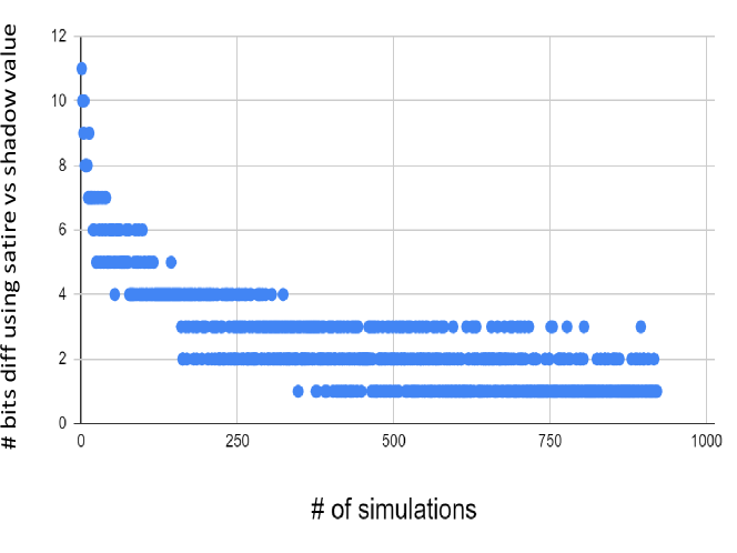
Figure 3: Difference in precision estimate(# bits lost) between Satire and shadow value calculation

Even for shadow-value evaluations, one uses a high-precision value as a proxy for the “true value.” Let $f_{dp}$ and $f_{qp}$ denote the observed values when using double and quad (high) precision, respectively. In figure 3, the y-axis plots the prediction difference, $Q$, evaluated as shown in equation$~{}\eqref{eq:compare-rel-error}$ and the x-axis plots the simulations done for the empirical evaluation. Here $qsat$, the numerator, is from Satire’s worst case-bounds, the denominator is the observed value in the working precision (here, double). For $qshadow$, the numerator is the observed difference in dynamic data between double and quad precision values, while its denominator is the quad precision value.

In practice, using shadow-value calculations is a large burden for the user: an entirely duplicated thread has to be run in high precision, with additional necessary code changes. Our objective is to help the user avoid all this and still allow them to gain value through Satire’s analysis toward precision loss. We aim to show that using only the observed values, we can precisely inform the loss in precision bits. In other words, $Q$ should be always greater than zero for soundness but close to zero for tightness. Figure 3 shows denser regions closer to zero implying the tightness of our analysis compared to the shadow value calculation, while never crossing zero indicating a sound bound. Thus, we believe that users can use Satire’s analysis to obtain a quick indication of precision loss—at least in a relative sense. That is, they may be able to use our methods to zoom into code regions that have higher loss and improve overall higher precision.

7 Additional Related Work

Precision analysis plays an important role in safety-critical systems. For trustworthy error analysis formally certified bounds are needed, and some recent examples are [3, 47].

Rosa and FPTaylor are the closest to our work in their approach to extend Taylor forms rigorous floating point error estimation. Rosa propagates errors in numeric affine form and uses SMT solvers to obtain tight bounds. In FPTaylor, full symbolic Taylor forms are obtained and fed to a global optimizer, which often results in large expressions, impeding scalability. In contrast, Satire’s decoupled analysis achieves the same end-result albeit without this complexity, by using a forward and backward pass that greatly improves overall effectiveness.

While scalability has been previously achieved, it required manual assistance using abstract interpretation [10] coupled with theorem proving (e.g., FLuctuat [14, 6]). Gappa [13] is basically an interval-based reasoning system, but comes with many simplification rules of its own, and has been embedded into verifiers such as [17] and various proof-assistants [34, 23, 49]. Combined uses of static analyses [20] are popular, as demonstrated at scale in Astrée [11]. A general abstract domain for floating-point computations is described in [32].

The importance of sound techniques for relative error estimation has been recognized by many. A common approach for relative error estimation is to first obtain the absolute error and then divide it by the minimum of the function interval value. A combined rigorous approach to relative error estimation is presented in [25]. Our approach for relative error estimation is meant for use in a dynamic analysis setting. It is motivated by the important pragmatic consideration of avoiding shadow-value computations on an existing piece of code. We use the observed value at runtime in combination with Satire’s worst-case bound to obtain a relative error profile that provides insights on precision loss. Through empirical evaluation, we establish the reliability of this approach.

8 Concluding Remarks

We presented Satire, a tool for rigorous floating-point error analysis that produces tight error bounds in practice. Satire is similar to many of its predecessors, but specifically emphasizes handling large expressions that arise in practice by including an information-theoretic abstraction mechanism for scalability. The effectiveness of Satire has been demonstrated on practical examples including FFT, parallel prefix sum, and stencils for various partial differential equation (PDE) types. Even divergent families of equations such as the Lorenz system are included in our study. Satire can provide insights on the loss of precision at runtime as demonstrated on a large ill-conditioned problem. We believe this variety and scale in an automated rigorous tool is unique.

Our work quickly showed us that rather than merely the size of expressions, one must also take the kinds of computations being analyzed. For instance, very large expressions generated by FDTD and heat-flow can be analyzed without using abstractions for large sizes; however, highly non-linear systems such as Lorenz require abstractions even for small sizes.

An important conclusion that emerges pertains to the impact of losing variable correlations due to abstractions: it is an important consideration in choosing when and where to abstract. The importance of incremental and decoupled error expression computation is also brought out. Given that global optimizers are workhorses in error estimation, our studies shed light on the role of expression canonicalization. This fits well with incremental computation, allowing global optimizer calls to be smaller as well as can be parallelized.

Important future directions include handling loops (enabling further scaling), improving abstractions without increasing error bounds, and the use of parallelism to further speed up the analysis.

References

- [1] Alliot, J.M., Durand, N., Gianazza, D., Gotteland, J.B.: Finding and proving the optimum: Cooperative stochastic and deterministic search. In: Proceedings of the 20th European Conference on Artificial Intelligence (ECAI). pp. 55–60. ACM (2012). https://doi.org/10.3233/978-1-61499-098-7-55
- [2] Altman, M., Gill, J., McDonald, M.P.: Numerical Issues in Statistical Computing for the Social Scientist. John Wiley & Sons, Inc. (Dec 2003). https://doi.org/10.1002/0471475769, https://doi.org/10.1002/0471475769
- [3] Becker, H., Zyuzin, N., Monat, R., Darulova, E., Myreen, M., Fox, A.: A verified certificate checker for finite-precision error bounds in coq and hol4. In: FMCAD. pp. 1–10 (10 2018). https://doi.org/10.23919/FMCAD.2018.8603019
- [4] Bischof, C., Buker, H., Hovland, P., Naumann, U., Utke, J. (eds.): Advances in Automatic Differentiation. Springer (2008), iSBN : 978-3-540-68935-5
- [5] Boldo, S., Clément, F., Filliâtre, J.C., Mayero, M., Melquiond, G., Weis, P.: Wave equation numerical resolution: A comprehensive mechanized proof of a c program. Journal of Automated Reasoning 50(4), 423–456 (Aug 2012). https://doi.org/10.1007/s10817-012-9255-4, https://doi.org/10.1007/s10817-012-9255-4
- [6] Boldo, S., Clément, F., Filliâtre, J.C., Mayero, M., Melquiond, G., Weis, P.: Wave equation numerical resolution: A comprehensive mechanized proof of a C program. Journal of Automated Reasoning (JAR) 50(4), 423–456 (2013). https://doi.org/10.1007/s10817-012-9255-4
- [7] Brent, R.P., Percival, C., Zimmermann, P.: Error bounds on complex floating-point multiplication. Math. Comput. 76, 1469–1481 (2007)
- [8] Brisebarre, N., Joldes, M., Muller, J.M., Naneş, A.M., Picot, J.: Error analysis of some operations involved in the Cooley-Tukey Fast Fourier Transform. ACM Transactions on Mathematical Software pp. 1–34 (2019)
- [9] Chiang, W.F., Baranowski, M., Briggs, I., Solovyev, A., Gopalakrishnan, G., Rakamariundefined, Z.: Rigorous floating-point mixed-precision tuning. SIGPLAN Not. 52(1), 300–315 (Jan 2017). https://doi.org/10.1145/3093333.3009846, https://doi.org/10.1145/3093333.3009846
- [10] Cousot, P., Cousot, R.: Abstract interpretation: A unified lattice model for static analysis of programs by construction or approximation of fixpoints. In: Proceedings of the 4th ACM SIGACT-SIGPLAN Symposium on Principles of Programming Languages (POPL). pp. 238–252. ACM (1977)
- [11] Cousot, P., Cousot, R., Feret, J., Mauborgne, L., Miné, A., Monniaux, D., Rival, X.: The ASTRÉE analyser. In: Proceedings of the 14th European Symposium on Programming Languages and Systems (ESOP). Lecture Notes in Computer Science, vol. 3444, pp. 21–30. Springer (2005)
- [12] Darulova, E., Kuncak, V.: Sound compilation of reals. In: Proceedings of the 41st ACM SIGPLAN-SIGACT Symposium on Principles of Programming Languages (POPL). pp. 235–248. ACM (2014)
- [13] Daumas, M., Melquiond, G.: Certification of Bounds on Expressions Involving Rounded Operators. ACM Transactions on Mathematical Software 37(1), 1–20 (2010)
- [14] Delmas, D., Goubault, E., Putot, S., Souyris, J., Tekkal, K., Védrine, F.: Towards an Industrial Use of FLUCTUAT on Safety-Critical Avionics Software. In: Formal Methods for Industrial Critical Systems, FMICS 2009, Lecture Notes in Computer Science, vol. 5825, pp. 53–69. Springer Berlin Heidelberg (2009). https://doi.org/10.1007/978-3-642-04570-7_6
- [15] Denis, C., de Oliveira Castro, P., Petit, E.: Verificarlo: Checking floating point accuracy through monte carlo arithmetic. In: Montuschi, P., Schulte, M.J., Hormigo, J., Oberman, S.F., Revol, N. (eds.) 23nd IEEE Symposium on Computer Arithmetic, ARITH 2016, Silicon Valley, CA, USA, July 10-13, 2016. pp. 55–62. IEEE Computer Society (2016). https://doi.org/10.1109/ARITH.2016.31, https://doi.org/10.1109/ARITH.2016.31
- [16] FPBENCH, benchmarks, compilers and standards for the floating point research community. http://fpbench.org/benchmarks.html
- [17] Frama-C Software Analyzers. http://frama-c.com/index.html (2017)
- [18] Gelpia: A global optimizer for real functions (2017), https://github.com/soarlab/gelpia
- [19] Goodloe, A.E., Muñoz, C., Kirchner, F., Correnson, L.: Verification of numerical programs: From real numbers to floating point numbers. In: Brat, G., Rungta, N., Venet, A. (eds.) NASA Formal Methods. pp. 441–446. Springer Berlin Heidelberg, Berlin, Heidelberg (2013)
- [20] Goubault, E., Putot, S.: Static Analysis of Finite Precision Computations. In: International Workshop on Verification, Model Checking, and Abstract Interpretation, VMCAI 2011, Lecture Notes in Computer Science, vol. 6538, pp. 232–247. Springer Berlin Heidelberg (2011)
- [21] Guo, H., Rubio-González, C.: Exploiting community structure for floating-point precision tuning. In: ISSTA. pp. 333–343 (07 2018). https://doi.org/10.1145/3213846.3213862
- [22] Harrison, J.: A machine-checked theory of floating point arithmetic. In: Bertot, Y., Dowek, G., Hirschowitz, A., Paulin, C., Théry, L. (eds.) Theorem Proving in Higher Order Logics: 12th International Conference, TPHOLs’99. Lecture Notes in Computer Science, vol. 1690, pp. 113–130. Springer-Verlag, Nice, France (1999)
- [23] Harrison, J.: Floating-Point Verification Using Theorem Proving. In: SFM 2006, Lecture Notes in Computer Science, vol. 3965, pp. 211–242. Springer Berlin Heidelberg (2006)
- [24] Higham, N.J.: Accuracy and Stability of Numerical Algorithms. Society for Industrial and Applied Mathematics, second edn. (2002). https://doi.org/10.1137/1.9780898718027, https://epubs.siam.org/doi/abs/10.1137/1.9780898718027
- [25] Izycheva, A., Darulova, E.: On sound relative error bounds for floating-point arithmetic. In: Proceedings of the 17th Conference on Formal Methods in Computer-Aided Design. p. 15–22. FMCAD ’17, FMCAD Inc, Austin, Texas (2017)
- [26] Jacquemin, M., Putot, S., Védrine, F.: A reduced product of absolute and relative error bounds for floating-point analysis. In: Podelski, A. (ed.) Static Analysis - 25th International Symposium, SAS 2018, Freiburg, Germany, August 29-31, 2018, Proceedings. Lecture Notes in Computer Science, vol. 11002, pp. 223–242. Springer (2018). https://doi.org/10.1007/978-3-319-99725-4_15, https://doi.org/10.1007/978-3-319-99725-4_15
- [27] Jr, E., Saleh, H.: Fft implementation with fused floating-point operations. Computers, IEEE Transactions on 61, 284 – 288 (03 2012). https://doi.org/10.1109/TC.2010.271
- [28] Lam, M.O., Hollingsworth, J.K.: Fine-grained floating-point precision analysis. The International Journal of High Performance Computing Applications 32(2), 231–245 (Jun 2016). https://doi.org/10.1177/1094342016652462, https://doi.org/10.1177/1094342016652462
- [29] Lee, W., Sharma, R., Aiken, A.: On automatically proving the correctness of math.h implementations. PACMPL 2(POPL), 47:1–47:32 (2018). https://doi.org/10.1145/3158135, https://doi.org/10.1145/3158135
- [30] Liang, J., Song, W.: Difference equation of lorenz system. International Journal of Pure and Apllied Mathematics 83 (02 2013). https://doi.org/10.12732/ijpam.v83i1.9
- [31] Magron, V., Constantinides, G., Donaldson, A.: Certified roundoff error bounds using semidefinite programming. ACM Transactions on Mathematical Software 43(4), 34:1–34:31 (Jan 2017). https://doi.org/10.1145/3015465, http://doi.acm.org/10.1145/3015465
- [32] Martel, M.: Semantics of roundoff error propagation in finite precision calculations. Higher Order Symbolic Computation 19(1), 7–30 (2006). https://doi.org/10.1007/s10990-006-8608-2, http://dx.doi.org/10.1007/s10990-006-8608-2
- [33] Mccullough, B.D., Vinod, H.: The numerical reliability of econometric software. Journal of Economic Literature 37, 633–665 (02 1999). https://doi.org/10.1257/jel.37.2.633
- [34] Melquiond, G.: Floating-Point Arithmetic in the Coq System. Information and Computation 216, 14–23 (2012). https://doi.org/10.1016/j.ic.2011.09.005, http://dx.doi.org/10.1016/j.ic.2011.09.005
- [35] Menon, H., Lam, M.O., Osei-Kuffuor, D., Schordan, M., Lloyd, S., Mohror, K., Hittinger, J.: Adapt: Algorithmic differentiation applied to floating-point precision tuning. In: Proceedings of the International Conference for High Performance Computing, Networking, Storage, and Analysis. SC ’18, IEEE Press (2018)
- [36] Moscato, M.M., Titolo, L., Feliú, M.A., Muñoz, C.A.: Provably correct floating-point implementation of a point-in-polygon algorithm. In: ter Beek, M.H., McIver, A., Oliveira, J.N. (eds.) Formal Methods – The Next 30 Years. pp. 21–37. Springer International Publishing, Cham (2019)
- [37] Narkawicz, A., Muñoz, C., Dutle, A.: Formally-verified decision procedures for univariate polynomial computation based on sturm’s and tarski’s theorems. Journal of Automated Reasoning 54(4), 285–326 (Feb 2015). https://doi.org/10.1007/s10817-015-9320-x, https://doi.org/10.1007/s10817-015-9320-x
- [38] Panchekha, P., Sanchez-Stern, A., Wilcox, J.R., Tatlock, Z.: Automatically improving accuracy for floating point expressions. In: Proceedings of the 36th ACM SIGPLAN Conference on Programming Language Design and Implementation, PLDI 2015. pp. 1–11. ACM (2015). https://doi.org/10.1145/2737924.2737959, http://doi.acm.org/10.1145/2737924.2737959
- [39] Failure of the Patriot Missle due to Floating-Point Error Accumulation. http://www.ima.umn.edu/~arnold/455.f96/disasters.html
- [40] Percival, C.: Rapid multiplication modulo the sum and difference of highly composite numbers. Math. Comput. 72(241), 387395 (Jan 2003). https://doi.org/10.1090/S0025-5718-02-01419-9, https://doi.org/10.1090/S0025-5718-02-01419-9
- [41] Ramos, G.: Roundoff error analysis of the fast fourier transform. Mathematics of Computation - Math. Comput. 25, 757–757 (10 1971). https://doi.org/10.1090/S0025-5718-1971-0300488-0
- [42] Rubio-González, C., Nguyen, C., Nguyen, H.D., Demmel, J., Kahan, W., Sen, K., Bailey, D.H., Iancu, C., Hough, D.: Precimonious: Tuning assistant for floating-point precision. In: Supercomputing (SC). pp. 27:1–27:12 (2013), https://github.com/corvette-berkeley/precimonious
- [43] Salvia, R., Titolo, L., Feliú, M.A., Moscato, M.M., Muñoz, C.A., Rakamaric, Z.: A mixed real and floating-point solver. In: Badger, J.M., Rozier, K.Y. (eds.) NASA Formal Methods - 11th International Symposium, NFM 2019, Houston, TX, USA, May 7-9, 2019, Proceedings. Lecture Notes in Computer Science, vol. 11460, pp. 363–370. Springer (2019). https://doi.org/10.1007/978-3-030-20652-9_25, https://doi.org/10.1007/978-3-030-20652-9_25
- [44] Schkufza, E., Sharma, R., Aiken, A.: Stochastic Optimization of Floating-point Programs with Tunable Precision. In: PLDI 2014. pp. 53–64. PLDI ’14, ACM (2014)
- [45] Shannon, C.E.: A mathematical theory of communication. The Bell System Technical Journal 27(3), 379–423 (7 1948). https://doi.org/10.1002/j.1538-7305.1948.tb01338.x, https://ieeexplore.ieee.org/document/6773024/
- [46] Simengine. https://www.ensoftcorp.com/simengine/
- [47] Solovyev, A., Baranowski, M.S., Briggs, I., Jacobsen, C., Rakamaric, Z., Gopalakrishnan, G.: Rigorous estimation of floating-point round-off errors with symbolic taylor expansions. ACM Trans. Program. Lang. Syst. 41(1), 2:1–2:39 (2019). https://doi.org/10.1145/3230733, https://doi.org/10.1145/3230733
- [48] Stolfi, J., de Figueiredo, L.H.: An Introduction to Affine Arithmetic. TEMA Trends in Applied and Computational Mathematics 4(3), 297–312 (2003)
- [49] Titolo, L., Feliú, M.A., Moscato, M., Muñoz, C.A.: An abstract interpretation framework for the round-off error analysis of floating-point programs. In: Lecture Notes in Computer Science, pp. 516–537. Springer International Publishing (Dec 2017). https://doi.org/10.1007/978-3-319-73721-8_24, https://doi.org/10.1007/978-3-319-73721-8_24