MolTrans: Molecular Interaction Transformer for Drug Target Interaction Prediction
Abstract
Motivation: Drug target interaction (DTI) prediction is a foundational task for in silico drug discovery, which is costly and time-consuming due to the need of experimental search over large drug compound space. Recent years have witnessed promising progress for deep learning in DTI predictions. However, the following challenges are still open: (1) the sole data-driven molecular representation learning approaches ignore the sub-structural nature of DTI, thus produce results that are less accurate and difficult to explain; (2) existing methods focus on limited labeled data while ignoring the value of massive unlabelled molecular data.
Results: We propose a Molecular Interaction Transformer (MolTrans) to address these limitations via: (1) knowledge inspired sub-structural pattern mining algorithm and interaction modeling module for more accurate and interpretable DTI prediction; (2) an augmented transformer encoder to better extract and capture the semantic relations among substructures extracted from massive unlabeled biomedical data. We evaluate MolTrans on real world data and show it improved DTI prediction performance compared to state-of-the-art baselines.
Availability: The model scripts and weights will be open sourced at Github.
Contact: jimeng@illinois.edu
keywords:
Drug-Target Interaction Prediction; Deep Learning; Drug Discovery.1 Introduction
Drug discovery is notoriously costly and time-consuming due to the need of experimental search over large drug compound space. Take its key task, drug-target protein interaction (DTI) prediction as an example. DTI serves as the foundation for finding new drugs (i.e., virtual screening) and new indications of existing drugs (i.e., drug repositioning), since the therapeutic effects of drug compounds are detected by examining DTIs [1]. During the compound identification process, researchers often need to conduct assay experiments and search over 97M possible compounds in a candidate database [2].
Luckily, with massive biomedical data and knowledge being collected and available, along with the advances of deep learning technologies which demonstrated huge success in many application areas, the drug discovery process particularly DTI prediction has been significantly enhanced. Recently, various deep models have shown encouraging performance in DTI predictions. They often take drug and protein data as inputs, cast DTI as a classification problem, and make prediction by feeding the inputs through deep learning models such as deep neural network (DNN) [3], deep belief network (DBN) [4], and convolutional neural network (CNN) [5, 6, 7]. Despite these efforts, the following challenges are still open.
-
1.
Inadequate modeling of interaction mechanism. Existing works [6, 7, 8] learn molecular representation and make prediction based on whole molecular structure of drugs and proteins, ignoring that the interactions are sub-structural– only involving relevant sub-structures of drugs and proteins [9, 10]. The full-structural molecular representations introduce noises and affect the prediction performance. Also, the learned representations are hard to interpret since they do not provide a tractable path to indicate which sub-structures of drugs and proteins contribute to the interactions.
-
2.
Restricted to limited labeled data. Previous works [6, 7, 8, 11, 4] focus on data in hand and limit the scope within several thousands of drugs and proteins while ignoring the vast (e.g., order of millions) unlabelled biomedical data available. The model architectures in previous works also are not designed to enable the integration of massive dataset.
To solve these challenges, we propose a transformer [12]-based bio-inspired molecular data representation method (coined as MolTrans) to leverage vast unlabelled data for in silico DTI prediction.
MolTrans is enabled by the following technical contributions:
-
1.
Knowledge inspired representation and interaction modeling for more accurate and explainable prediction. Inspired by the knowledge that DTI is sub-structural, MolTrans derives a data-driven method called Frequent Consecutive Sub-sequence (FCS) mining that is adaptable to extract high-quality fit-sized sub-structures for both protein and drug. In addition, MolTrans includes a bio-inspired interaction module imitating the real biological DTI process. The new sub-structure fingerprints enable a tractable path for understanding which sub-structure combination has more relevance to the outcome through an explicit map in the interaction module.
-
2.
Leverage massive unlabelled biomedical data. MolTrans mines through millions of drugs and proteins sequences from multiple unlabelled data sources to extract high quality sub-structures of drugs and proteins. The vast data result in a much higher quality sub-structures than using small training dataset alone. We also augment the representation using transformers [12], which captures the complex signals among the large sequential sub-structures outputs generated from the unlabelled data.
We provide a comprehensive performance comparison of state-of-the-art methods on various realistic drug discovery settings include unseen drug/target problems and in scarce training dataset setup. We show empirically that MolTrans has robust improved predictive performance over state-of-the-art baselines.
2 Related Works
Numerous computational methods have been developed for DTI prediction problem. Similarity-based methods such as kernel regression [13] and matrix factorization [14] methods exploit known DTI’s drug-target similarity information and infer new ones. However, these methods are shown to be not generalizable to different protein classes [4]. Feature-based methods feed numerical descriptors of drug and proteins into downstream prediction models. Popular numerical descriptors include ECFP [15] and PubChem [16] for drugs, CTD [17] and PSC [18] for proteins. Classic machine learning methods such as gradient boosting [19] have shown promises in predictive performance. Recently, deep learning based methods [3, 4, 6, 20] have shown further improvement of performance due to its capability to capture complex non-linear signals of DTI. MolTrans differs from existing works with (1) its knowledge-driven model architecture design rather than direct application of existing deep learning models; (2) emphasis on interpretability instead of predictive performance alone to potentially aid medical chemists for better decision making; (3) usage of external drug and target data to complement interaction dataset.
3 Method
3.1 Problem Definition
We formulate the DTI prediction as a classification task to determine whether a pair of drug and target protein will interact. In our setting, drug is represented by the Simplified Molecular Input Line Entry System (SMILES) , which consists of a sequence of chemical atoms and bonds tokens (e.g. C, O, S), generated by depth-first traversal over the molecule graph. We denote for drug’s SMILES representation. Target protein, denoted as , is represented by a sequence of protein tokens, where each token is one of the 23 amino acids. The DTI prediction task is defined as below.
Problem 1 (Drug Target Interaction (DTI) Prediction).
Given compound sequence for drugs and protein sequence for proteins, the DTI prediction task can be casted as to learn a function mapping from drug-target pairs to an interaction probability score.
Notations Description drug SMILES, protein amino acids the set of interacting/non-interacting DTI pairs entire sub-structures set for protein and drug sub-structures set in one pair of drug-target one-hot input representation for protein one-hot input representation for drug latent representation for protein latent representation for drug the interaction tensor ; the interaction function; interaction probability the output of interaction module the weight for content embedding protein the weight for content embedding drug the weight for position embedding protein the weight for position embedding drug the weight, bias for decoder
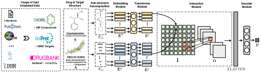
3.2 The MolTrans Method
The MolTrans framework learns to predict DTI as follows. Given the input drug and protein data, a frequent consecutive sub-sequence mining module first decomposes them into a set of explicit sequences of sub-structures using a specialized decomposition algorithm with inputs consisting of vast unlabelled data. The outputs are then fed into a augmented transformer embedding module to obtain an augmented contextual embedding for each sub-structure through transformer encoders [12]. Next, in the interaction prediction module, drug sub-structures are paired with protein sub-structures with pairwise interaction scores. A CNN layer is later applied on the interaction map to capture higher-order interactions. Finally, a decoder module outputs a score indicating the probability of pairwise interactions.
3.2.1 Frequent Consecutive Sub-sequence Mining Module
Driven by the domain knowledge that DTI happens in a sub-structural level, MolTrans first decomposes molecular sequence for proteins and drugs into sub-structures. In particular, we propose a data-driven sequential pattern mining algorithm called Frequent Consecutive Sub-sequence Algorithm () to find recurring sub-sequences across drug and protein databases. Inspired by the invention of sub-word units in the natural language processing field [21, 22], aims to generate a set of hierarchy of frequent sub-sequences for sequences. The algorithm is summarized in Algo. Using algorithm, MolTrans converts input drug and target to a sequence of explicit sub-structures and respectively. The significance of is two-folds:
-
1.
It distinguishes from previous sub-structure fingerprinting methods as it is more explainable. Commonly used fingerprint such as ECFP [15] is not explainable due to its hashing nature. Explicit sub-structure fingerprint such as PubChem encoding has on average 100 granular sub-structures for a small molecule where many sub-structures are a subset of other ones, making it intractable to know which sub-structure leads to the outcome. In contrast, FCS drug encoding is capable of giving explicit hints as it decomposes each drug molecule into discrete and moderate size partitions of sub-structures as shown in Sec. 4.6.
-
2.
It allows for leveraging the massive unlabelled data for improved sub-structure mining. For example, we use the Uniprot dataset [23] consists of 560,823 unique protein sequences and the ChEMBL database [24] which includes 1,870,461 drug SMILES strings. We observe that the quality of the mined sub-structures originates from the massive unlabelled data we used. In small datasets, the occurrences of many useful sub-structures are below the reasonable minimum frequency whereas a large aggregation dataset can successfully identify them with a larger sequences pool. We also show that the encoding has better predictive power when using massive unlabelled data compared to using small datasets, in Sec. 4.7.
3.2.2 Augmented Transformer Embedding Module
To capture the chemical semantics of sub-structures, MolTrans includes an augmented embedding module where it first initializes a learn-able sub-structure look-up dictionary and then augment the embedding with the contextual sub-structural information via transformer encoders [12].
Concretely, for each input drug-target pair, we transform the corresponding sequence of sub-structures and into two matrices and where is the total size of sub-structures for drug/protein or the cardinality of the vocabulary set from FCS algorithm, and are the maximum lengths of sub-structure sequences for protein and drug, and each column and is a one-hot vector corresponding to the sub-structure index for the -th sub-structure of protein sequence and -th sub-structure of drug sequence. The content embedding for each protein and drug is generated via a learnable dictionary lookup matrix and such that
| (1) |
where is the size of latent embedding for each sub-structure.
Since MolTrans uses sequential sub-structures, we also include a positional embedding via a lookup dictionary [12] and :
| (2) |
where is a single hot vector where th position is 1.
The final embedding are generated via the sum of content and positional embedding:
| (3) |
The models above outputs a set of independent sub-structure embedding. However, these sub-structures have chemical relationships (e.g. Octet rules) among themselves to capture these contextual information, we further augment the embedding using a transformer encoder layers [12]:
| (4) |
Transformer encoder is ideal in our case because in the core of a transformer encoder, it is a series of self-attention head that modify each individual sub-structure embedding by learning the distribution of the effects from all the other sub-structures.
3.2.3 Interaction Prediction Module
MolTrans includes an interaction module that consists of two layers: (a) an interaction tensor to model pair-wise sub-structural interaction; (b) a CNN layer over interaction map to extract neighborhood interaction.
Pairwise interaction. To model the pairwise interaction, for each sub-sequence in protein and sub-sequence in drug, we have
| (5) |
where is a function that measures the interaction between the pairs. It can be any function such as sum, average, and dot product. Therefore, after this layer, we have a tensor where is the length of sub-sequences for drug/protein respectively, and is the size of the output of function , where Each column in this tensor takes account into the interaction of individual sub-structure of proteins and drugs. To provide explainability, we favor dot product as the aggregation function because it generates a single scalar that explicitly measures the intensity of interaction between individual target-drug sub-structural pair. As dot product output is one dimensional for every pair, becomes a two-dimensional interaction map. By examining this map, we directly see which sub-structure pairs contribute to the final outcome.
Neighborhood interaction. Nearby sub-structure of proteins and drugs influence each other in triggering the interactions. Hence, besides modeling the individual pair-wise interaction, it is also necessary to model the interaction to the nearby regions. We achieve this through a Convolutional Neural Network (CNN) [25] layer on top of the interaction map . The intuition is that by applying several order-invariant local convolution filters, interaction to nearby regions can be captured and aggregated. We obtain the output representation of the input drug-target pair:
| (6) |
This interaction module is inspired from the Deep Interactive Inference Network [26]. Thanks to this explicit interaction modeling, we can later visualize the strength of individual sub-structural interaction pair from the interaction map. To output a probability indicating the likelihood of interaction, we first flatten the into a vector and use a linear layer parametrized by weight matrix and bias vector :
| (7) |
where .
The entire network with parameters , , , , , the Transformer Encoders weights and CNN weights can be jointly optimized through the binary classification loss:
| (8) |
where is the ground truth label.
4 Experiment
We design experiments to answer the following questions.
-
Q1
: Does MolTrans improve DTI predictive performance?
-
Q2
: How well does MolTrans tackle the unseen-drug/target cases?
-
Q3
: How does MolTrans respond to large number of missing data?
-
Q4
: Does MolTrans provide useful knowledge about DTI?
-
Q5
: How does each component of MolTrans contribute to the predictive performance gain?
4.1 Experimental Setup
Dataset. We use the MINER DTI dataset from BIOSNAP collection [27]. It consists of 4,503 drug nodes and 2,182 protein targets, and 15,138 drug-target interaction pairs from DrugBank [28]. BIOSNAP dataset only contains positive drug target interaction pairs. For negative pairs, we sample from the unseen pairs. We obtain a balanced dataset with equal positive and negative samples. We use Uniprot database to obtain target sequence and DrugBank database to obtain SMILES strings, and hence, we filter out target/drug that do not have target sequences/SMILES from Uniprot/DrugBank.
Metrics. We use ROC-AUC (Area under the receiver operating characteristic curve) and PR-AUC (Area under the precision-recall curve) as metrics to measure the binary classification performance.
Evaluation Strategies. We divided the dataset into training, validation and testing sets in a 7:1:2 ratio. For every experiment, we conduct five independent runs with different random splits of dataset. We then select the best performing model based on ROC-AUC performance from the validation set. The selected model via validation is then evaluated on the test set with the result reported below.
Implementation Details. MolTrans is implemented in PyTorch [29]. For experiments, we use a server with 2 Intel Xeon E5-2670v2 2.5GHZ CPUs, 128GB RAM and 2 NVIDIA Tesla P40 GPUs. For MolTrans, we use Adam optimizer with learning rate of 1e-5. We set the batch size to be 64 and we allow it to run for 30 epochs. It converges between 8-15 epochs. The input embedding is of size 384 and we set 12 attention heads for each transformer encoder with intermediate dimension 1,536. The dropout rate is 0.1. We set the maximum length of sequence for both drug and protein to cover 95 of drugs and proteins in the dataset. For the CNN, we use three filters with kernel size three.
| Method | ROC-AUC | PR-AUC |
|---|---|---|
| KronRLS | ||
| LR | ||
| DNN | ||
| DeepDTI | ||
| DeepDTA | ||
| GNN-CPI | ||
| DeepConv-DTI | ||
| MolTrans |
4.2 Baselines
We compared MolTrans with the following baselines. We focus on state-of-the-art deep learning models as they have demonstrated superior performance over shallow models.
-
1.
KronRLS [13] applies a kernel least square method on the similarity matrix of drug and protein features.
-
2.
LR [18, 15] applies a logistic regression model on the concatenated drug and protein feature vectors. We experiment on all the combinations for ECFP4 [15] & PubChem [30] for drugs and protein sequence composition descriptor (PSC) [18] & Composition-Transition-Distribution (CTD) [17] for proteins. We find ECFP4 for drugs and PSC for protein has the highest performance.
-
3.
DNN uses a three layer deep neural network with hidden size 1,024 on top of the ECFP4 and PSC concatenated vector.
-
4.
DeepDTI [4] models DTI using Deep Belief Network [31], which is a stack of Restricted Boltzmann Machines [32]. It uses the concatenation of ECFP2, ECFP4, ECFP6 as the drug feature and uses PSC for protein features. We optimize the hyper-parameters described from the paper based on validation set performance.
-
5.
DeepDTA [7] applies CNN on both raw SMILES string and protein sequence to extract local residue patterns. The task is to predict binding affinity values. We add a Sigmoid activation function in the end to change it to a binary classification problem and we conduct hyper-parameter search to ensure fairness.
-
6.
GNN-CPI [20] uses graph neural network to encode drugs and use CNN to encode proteins. The latent vectors are then concatenated into a neural network for compound-protein interaction prediction. We follow the same hyper-parameter setting described in the paper.
-
7.
DeepConv-DTI [11] uses CNN and global max pooling layer to extract various length local pattern in protein sequence and applies fully connected layer on drug fingerprint ECFP4. It conducts extensive experiment on different datasets and is the state-of-the-art model in DTI binary prediction task. We follow the same hyper-parameter setting described in the paper.
4.3 Q1: MolTrans achieves superior predictive performance
To answer Q1, we randomly select 20 drug protein pairs as test set. Table. 2 shows MolTrans has better predictive baselines in the DTI prediction setting in both metrics.
4.4 Q2: MolTrans has competitive performance in unseen drug and target setting
To imitate the unseen drug/target task, we randomly select 20% drug/target proteins and all DTI pairs associated with these drugs and targets as the test set.
The results are in Fig. 2. We observe that KronRLS’s performance vary across settings. This is because KronRLS is a similarity-based method, hence it is susceptible to the data properties in hand. In the unseen drug setting, we find the one-layer LR is better than multi-layers DNN, and is worse than the SOTA methods with more complicated deep model design. This shows the necessity for carefully designed model architecture. We also see that MolTrans has competitive performance against the SOTA deep learning baselines in both settings.
4.5 Q3: MolTrans performs best with scarce data

Robust performance under scarce training dataset is ideal in DTI setting. We trained each method on 5%, 10%, 20%, and 30% of dataset and predict on the rest of them (we use 10% of the test edges as validation set for early stopping). The result is reported in Fig. 3. We see that MolTrans is the most robust method. In the contrast, SOTA baselines such as DeepDTI and DeepConv-DTI drop as missing fractions increase. One reason why MolTrans is good on scarce setting is that MolTrans leverages on embeddings from sub-structures which are relatively abundant hence transferable compared to other methods which utilize the entire drugs and proteins.
4.6 Q4: MolTrans allows model understanding
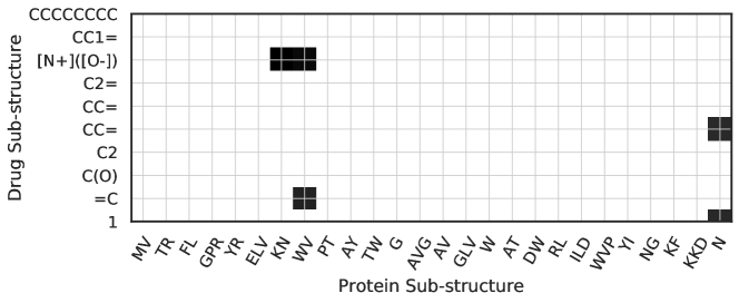
To answer Q4, we show through examples how the interaction map can provide hints on which sub-structure leads to the interaction. We first feed drug 2-nonyl n-oxide, and the protein Cytochrome b-c1 complex unit 1 into MolTrans, and we visualize the interaction map by filtering scalars that are larger than a threshold in Fig. 4. We saw the nitrogen oxide group [N+]([O-]) and KNWV has the highest interaction coefficient, matching with the previous study [33] who showed that nitrogen oxide group is essential for cytochrome inhibition activity. This example supports that MolTrans is capable of providing reasonable cues for understanding the model prediction and possibly shed light on the inner workings of DTI. To add more credibility, we feed Ephrin type-A receptor 4 (Epha4) target and Dasatinib drug into MolTrans, the map shows amino-thiazole group (S(=O)(=O) and N sub-structures) is highlighted with protein motif KF and DVG, which has an overlap with the Epha4-Dasatinib complex described in previous study [34]. We also feed the input target protein HDAC2 and the input drug hydroxamic acid. The interaction map assigns the NC(=O) group and the carbon chain with protein sub-structure KK, YG, DIG, DD with high intensity. The suggested ligand sub-structure matches with the observed interaction in HDAC2-SAHA co-complex [35].
4.7 Q5: Ablation Study
We conduct an ablation study on the full data setting with the following setup:
| Setup | ROC-AUC | PR-AUC |
|---|---|---|
| MolTrans | ||
| -CNN | ||
| -AugEmbed | ||
| -Interaction | ||
| Small | ||
| -FCS |
-
1.
-CNN: we remove the CNN from interaction module, and flatten the interaction map output and feed into the decoder.
-
2.
-AugEmbed: we remove the transformer in the augmented embedding module and feed the interaction module with the positional and content embedding,
-
3.
-Interaction: we further remove the interaction module from -AugEmbed. It degenerates to a decoder on top of the FCS fingerprint. Note that removing the interaction module alone is not a valid model design.
-
4.
Small: we use smaller dataset to train FCS: DrugBank for drug and BindingDB for protein. We adjust the minimal frequency to output a similar number of sub-structured as FCS-large.
-
5.
-FCS: we replace FCS with other popular drug/protein encoding. Here, we use ECFP4 for drug and PSC for protein.
From Table. 3, we see CNN, transformers and interaction module contribute to the model final performance. The FCS fingerprint alone has strong predictive performance already from -Interaction. In addition, from Small, we see the massive unlabelled data is useful as it enriches the input and boosts the performance. From -FCS, we see our model is adaptable to other popular fingerprints with similar strong performance (better than all SOTA baselines).
5 Conclusion
In this work, we introduce MolTrans, an end-to-end biological inspired deep learning based framework that models DTI process. We test under realistic drug discovery setting and evaluate with state-of-the-art baselines. We demonstrate empirically that MolTrans has competitive performance in accurately predicting DTI under all settings with an improved explainability.
References
- [1] J. P. Hughes, S. Rees, et al., Principles of early drug discovery, British journal of pharmacology 162 (6) (2011) 1239–1249.
- [2] J. R. Broach, J. Thorner, et al., High-throughput screening for drug discovery, Nature 384 (6604) (1996) 14–16.
- [3] T. Unterthiner, A. Mayr, et al., Deep learning as an opportunity in virtual screening, in: deep learning workshop at NIPS, Vol. 27, 2014, pp. 1–9.
- [4] M. Wen, Z. Zhang, et al., Deep-learning-based drug–target interaction prediction, JPR 16 (4) (2017) 1401–1409.
- [5] A. Mayr, G. Klambauer, T. Unterthiner, et al., Large-scale comparison of machine learning methods for drug target prediction on chembl, Chemical science 9 (24) (2018) 5441–5451.
- [6] H. Öztürk, E. Ozkirimli, A. Özgür, Widedta: prediction of drug-target binding affinity, arXiv preprint arXiv:1902.04166.
- [7] H. Öztürk, A. Özgür, E. Ozkirimli, Deepdta: deep drug–target binding affinity prediction, Bioinformatics 34 (17) (2018) i821–i829.
- [8] Y. Gao, A. Fokoue, et al., Interpretable drug target prediction using deep neural representation., in: IJCAI, 2018, pp. 3371–3377.
- [9] J. Jia, F. Zhu, et al., Mechanisms of drug combinations: interaction and network perspectives, Nature reviews Drug discovery 8 (2) (2009) 111.
- [10] M. Schenone, V. Dančík, et al., Target identification and mechanism of action in chemical biology and drug discovery, Nature chemical biology 9 (4) (2013) 232.
- [11] I. Lee, J. Keum, H. Nam, Deepconv-dti: Prediction of drug-target interactions via deep learning with convolution on protein sequences, PLoS computational biology 15 (6) (2019) e1007129.
- [12] A. Vaswani, N. Shazeer, et al., Attention is all you need, in: NIPS, 2017.
- [13] T. Pahikkala, A. Airola, et al., Toward more realistic drug–target interaction predictions, Briefings in bioinformatics 16 (2) (2014) 325–337.
- [14] X. Zheng, H. Ding, et al., Collaborative matrix factorization with multiple similarities for predicting drug-target interactions, in: KDD, 2013, pp. 1025–1033.
- [15] D. Rogers, M. Hahn, Extended-connectivity fingerprints, Journal of chemical information and modeling 50 (5) (2010) 742–754.
- [16] E. E. Bolton, Y. Wang, et al., Pubchem: integrated platform of small molecules and biological activities, in: Annual reports in computational chemistry, Vol. 4, Elsevier, 2008, pp. 217–241.
- [17] I. Dubchak, I. Muchnik, et al., Prediction of protein folding class using global description of amino acid sequence, PNAS 92 (19) (1995) 8700–8704.
- [18] D.-S. Cao, Q.-S. Xu, Y.-Z. Liang, propy: a tool to generate various modes of chou’s pseaac, Bioinformatics 29 (7) (2013) 960–962.
- [19] T. He, M. Heidemeyer, et al., Simboost: a read-across approach for predicting drug–target binding affinities using gradient boosting machines, Journal of cheminformatics 9 (1) (2017) 24.
- [20] M. Tsubaki, K. Tomii, J. Sese, Compound-protein interaction prediction with end-to-end learning of neural networks for graphs and sequences, Bioinformatics.
- [21] R. Sennrich, B. Haddow, A. Birch, Neural machine translation of rare words with subword units, arXiv:1508.07909.
- [22] P. Gage, A new algorithm for data compression, The C Users Journal 12 (2) (1994) 23–38.
- [23] E. Boutet, D. Lieberherr, et al., Uniprotkb/swiss-prot, in: Plant bioinformatics, Springer, 2007, pp. 89–112.
- [24] A. Gaulton, L. J. Bellis, et al., Chembl: a large-scale bioactivity database for drug discovery, Nucleic acids research 40 (D1).
- [25] A. Krizhevsky, I. Sutskever, G. E. Hinton, Imagenet classification with deep convolutional neural networks, in: Advances in neural information processing systems, 2012, pp. 1097–1105.
- [26] Y. Gong, H. Luo, J. Zhang, Natural language inference over interaction space, ICLR.
- [27] M. Zitnik, R. Sosič, et al., BioSNAP Datasets: Stanford biomedical network dataset collection (Aug. 2018).
- [28] D. Wishart, C. Knox, A. Guo, Drugbank: a knowledgebase for drugs, drug actions and drug targets., Nucleic Acids Research 36 (2008) 77.
- [29] A. Paszke, S. Gross, et al., Automatic differentiation in pytorch.
- [30] Y. Wang, J. Xiao, et al., Pubchem: a public information system for analyzing bioactivities of small molecules, Nucleic acids research 37 (suppl_2) (2009) W623–W633.
- [31] G. E. Hinton, Deep belief networks, Scholarpedia 4 (5) (2009) 5947.
- [32] G. E. Hinton, A practical guide to training restricted boltzmann machines, in: Neural networks: Tricks of the trade, Springer, 2012, pp. 599–619.
- [33] J. Lightbown, F. Jackson, Inhibition of cytochrome systems of heart muscle and certain bacteria by the antagonists of dihydrostreptomycin: 2-alkyl-4-hydroxyquinoline n-oxides, Biochemical Journal 63 (1) (1956) 130.
- [34] C. Farenc, P. H. Celie, et al., Crystal structure of the epha4 protein tyrosine kinase domain in the apo-and dasatinib-bound state, FEBS letters 585 (22) (2011) 3593–3599.
- [35] B. E. Lauffer, R. Mintzer, et al., Histone deacetylase (hdac) inhibitor kinetic rate constants correlate with cellular histone acetylation but not transcription and cell viability, Journal of Biological Chemistry 288 (37) (2013) 26926–26943.