Exceptional Points of Degeneracy Directly Induced by Space-Time Modulation of a Single Transmission Line

Abstract

We demonstrate how exceptional points of degeneracy (EPDs) are induced in a single transmission line (TL) directly by applying periodic space-time modulation to the per-unit-length distributed capacitance. In such space-time modulated (STM)-TL, two eigenmodes coalesce into a single degenerate one, in their eigenvalues (wavenumbers) and eigenvectors (voltage-current states) when the system approaches the EPD condition. The EPD condition is achieved by tuning a parameter in the space-time modulation, such as spatial or temporal modulation frequency, or the modulation depth. We unequivocally demonstrate the occurrence of the EPD by showing that the bifurcation of the wavenumber around the EPD is described by the Puiseux fractional power series expansion. We show that the first order expansion is sufficient to approximate well the dispersion diagram, and how this “exceptional” sensitivity of an STM-TL to tiny changes of any TL or modulation parameter enables a possible application as a highly sensitive TL sensor when operating at an EPD.

I Introduction

Recent advancements in EPD concepts have attracted a surge of interests due to their potential benefits in various electromagnetic applications. An EPD is a point in parameter space of a system at which multiple eigenmodes coalesce in both their eigenvalues and eigenvectors. The concept of EPD has been studied in lossless, spatially [1, 2, 3] or temporally [4] periodic structures, and in systems with loss and/or gain under parity-time symmetry [5, 6, 7, 8]. Since the characterizing feature of an exceptional point is the strong full degeneracy of at least two eigenmodes, as implied in [9], we stress the importance of referring to it as a “degeneracy”, hence of including the D in EPD. In essence, an EPD is obtained when the system matrix is similar to a matrix that comprises a non-trivial Jordan block [1, 10, 11, 12], here however the formulation leads to a matrix of infinite dimensions and therefore we assess the occurrence of the EPD by invoking the Puiseux fractional power expansion series [13] to describe the bifurcation of the dispersion diagram at the EPD. There are several features associated with the development of EPDs, which lead to applications, such as active systems gain enhancement in waveguides [14, 15, 16], and enhanced sensing [17, 18, 19, 20].

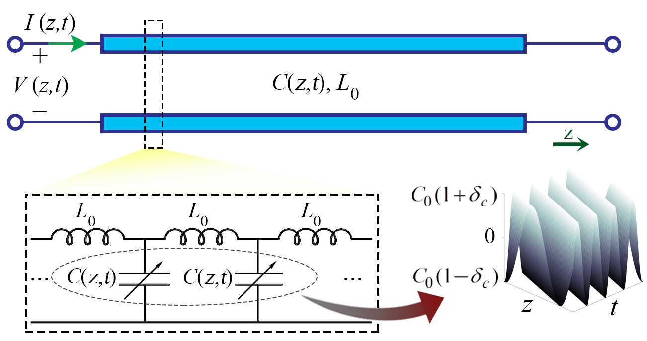
Figure 1: Schematic illustration of a single TL with space-time modulation of the distributed capacitance. We also show the equivalent TL circuit with the per-unit-length inductor and modulated capacitor.

Researchers have been studying how to incorporate time-variation of parameters into electromagnetic systems with the goal of adding new degrees of freedom in wave manipulation. In their pioneering work, Cassedy and Oliner studied the dispersion characteristics of wave propagation in a medium with dielectric constant modulated as a traveling-wave with sinusoidal form [21, 22]. Then, Elachi studied electromagnetic wave propagation and the wave vector diagram in general space-time periodic materials for different wave polarization [23]. In [24, 25], authors analyzed the reflection and transmission of an incident wave onto a time-periodic dielectric slab and generalize the concept of temporal photonic crystals to periodic modulation of the permeability and permittivity. In [26], magnetless nonreciprocity was demonstrated in spatiotemporally modulated coupled-resonator networks. Also, Taravati et al. proposed a mixer-duplexer-antenna leaky-wave system based on periodic space-time modulation [27]. Recently, in [28], space-time modulation was employed to control both phase and amplitude tunability in a metasurface, whereas traditionally metasurfaces have phase-only control on reflection/transmission. Several other papers have been published in recent years on time/space-time modulation to generate nonreciprocity in electromagnetic structures as [29, 30, 31, 32, 33]. In all these works, the concept of EPD in such modulated structures was not studied.

Here we leverage on the two concepts of space-time modulation and EPD and develop a general scheme to realize EPDs in space-time periodic, single TLs that can be used as a sensor or leaky wave antenna with ultra-high sensitivity. We investigate the occurrence of EPDs in a single TL when the per-unit-length capacitance is modulated in space and time, and we demonstrate its occurrence by showing that the bifurcation of the dispersion diagram around the EPD is well approximated by the Puiseux fractional power series expansion. This EPD-related fractional expansion is also used to explain the extreme sensitivity of the wavenumber to perturbation of system parameters.

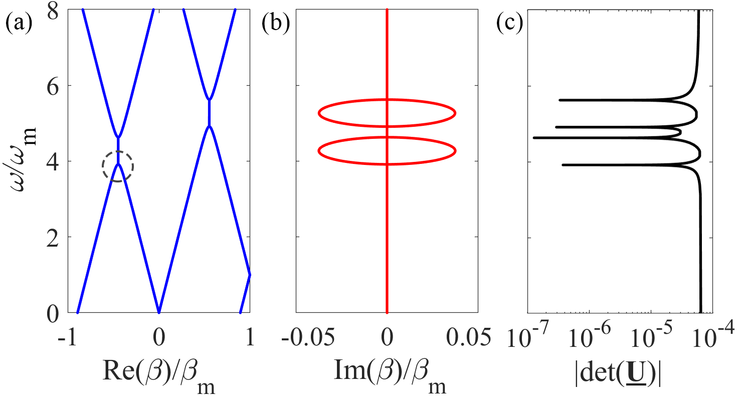
Figure 2: Dispersion diagram of the STM-TL with 2nd order EPDs. (a) Real part of the wavenumber of first harmonics and (b) the corresponding imaginary parts, and (c) plot of $\left|\mathrm{\mathrm{det}}(\underline{\mathbf{U}})\right|$ versus frequency. The similarity transformation matrix $\mathbf{\underline{U}}$ contains eigenvectors, therefore the vanishing of $\left|\mathrm{\mathrm{det}}(\underline{\mathbf{U}})\right|$ is necessary at an EPD.

II Degeneracies in a Uniform Single ST-MTL

Degeneracies in wave propagation in an infinitely long TL is examined when the per-unit-length capacitance is modulated in both space and time. We employ the formalism and description of a linear TL shown in [34]. A schematic representation of an STM-TL is shown in Fig. 1, where only the per-unit-length capacitance is space-time varying, while the per-unit-length inductance is constant throughout the TL. Without loss of generality we assume sinusoidal space-time variation; however, EPDs can be induced also by other forms of periodic space-time variation. The distributed per-unit-length space-time varying capacitance is given by

$$C(z,t)=C_{\mathrm{0}}+C_{m}(t)=C_{0}(1+\delta_{\mathrm{c}}\cos(\omega_{\mathrm{m}}t-\beta_{\mathrm{m}}z)),$$ (1)

where $C_{\mathrm{0}}$ is the space-time averaged (i.e., unmodulated) per-unit-length capacitance, $\delta_{\mathrm{c}}$ is the modulation depth, and $\omega_{\mathrm{m}}$ and $\beta_{\mathrm{m}}$ are the temporal and spatial modulation frequencies, respectively. The dynamic behavior of such a TL is captured using the Telegrapher’s equations, that are here represented in terms of a voltage and current state vector, $\boldsymbol{\boldsymbol{\Psi}}(z,t)=[\begin{array}[]{cc}V(z,t),&I(z,t)\end{array}]^{\mathrm{T}}$, where the superscript $\mathrm{T}$ denotes the transpose operation. The dynamic behavior of this state vector is described by the first order differential equations as

$$\partial_{\mathrm{z}}\boldsymbol{\boldsymbol{\Psi}}(z,t) = -\partial_{\mathrm{t}}\left(\underline{\mathbf{\underline{M}}}(z,t)\boldsymbol{\boldsymbol{\Psi}}(z,t)\right),$$ (2)

where the space-time modulated $2\times 2$ system matrix $\mathbf{\underline{\underline{M}}}$ is given by

$$\mathbf{\underline{\underline{M}}}(z,t)=\left[\begin{array}[]{cc}0&L_{\mathrm{0}}\\ C(z,t)&0\end{array}\right]\;.$$ (3)

We look for time-harmonic solutions, and because of the periodic nature of the modulation the state vector eigensolution is cast into an infinite space-time Floquet-Bloch series as

$$\boldsymbol{\boldsymbol{\Psi}}(z,t)=e^{j(\omega t-\beta z)}\stackrel{{\scriptstyle[}}{{q}}=-\infty]{\infty}{\sum}\mathbf{\boldsymbol{\boldsymbol{\Psi}}}_{q}\,e^{jq(\omega_{\mathrm{m}}t-\beta_{\mathrm{m}}z)},$$ (4)

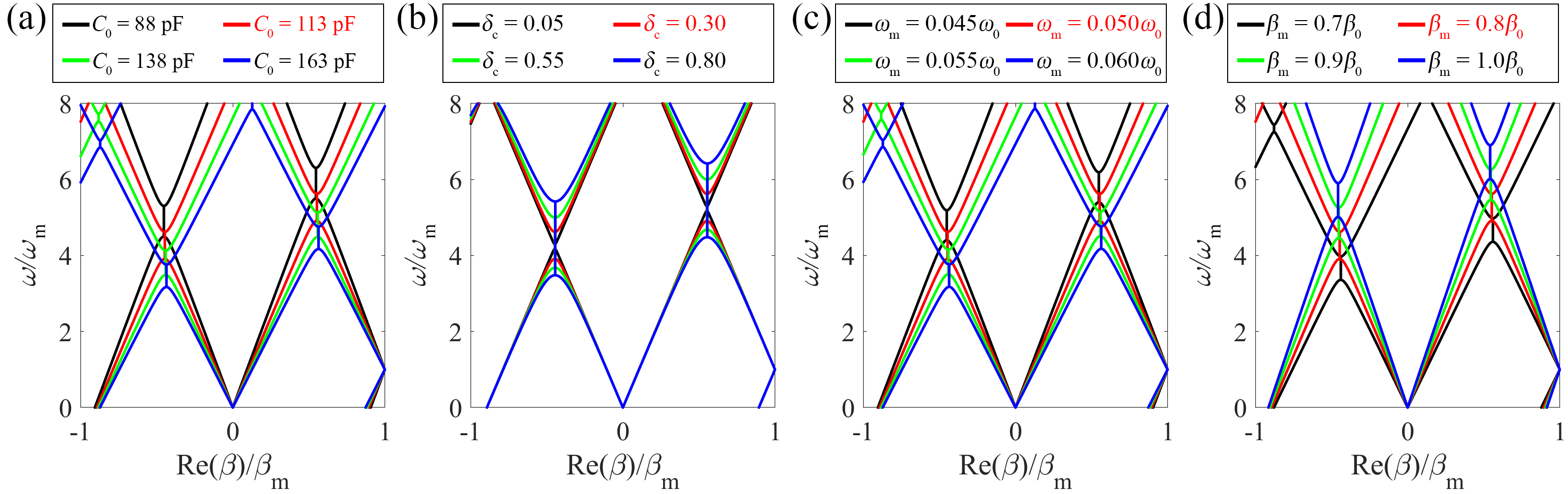
Figure 3: Dispersion diagrams of the real part of wavenumbers by changing one single parameter at the time. The system parameters that are changed are (a) $C_{\mathrm{0}}$, (b) $\delta_{\mathrm{c}}$, (c) $\omega_{\mathrm{m}}$, and (d) $\beta_{\mathrm{m}}$.

where $\beta$ and $\omega$ are the propagation wavenumber and the angular frequency, respectively, and $\boldsymbol{\boldsymbol{\Psi}}_{q}=[\begin{array}[]{cc}V_{q},&I_{q}\end{array}]^{\mathrm{T}}$ is the complex amplitude of the $q$-th harmonic of the state vector. We expand the space-time-varying distributed capacitance in Eq. (1) in terms of its Fourier series

$$C(z,t)=\stackrel{{\scriptstyle[}}{{s}}=-1]{1}{\sum}C_{s}\,e^{js(\omega_{\mathrm{m}}t-\beta_{\mathrm{m}}z)},$$ (5)

where $C_{s}$ represents the amplitude of the $s$-th harmonic. Substituting Eqs. (4) and (5) in Eq. (2) and taking the time and space derivatives, the equation for each $q$-th harmonics’ $\mathbf{\mathbf{\mathbf{\boldsymbol{\boldsymbol{\Psi}}}}}_{q}$ is obtained as

$$\begin{array}[]{c}\stackrel{{\scriptstyle[}}{{q}}=-\infty]{\infty}{\sum}(\beta+q\beta_{\mathrm{m}})\mathbf{\boldsymbol{\boldsymbol{\Psi}}}_{q}\,e^{jq(\omega_{\mathrm{m}}t-\beta_{\mathrm{m}}z)}=\\ \stackrel{{\scriptstyle[}}{{q}}=-\infty]{\infty}{\sum}\stackrel{{\scriptstyle[}}{{s}}=-1]{1}{\sum}\left[\begin{array}[]{cc}0&(\omega+q\omega_{\mathrm{m}})L_{\mathrm{0}}\delta_{s,\mathrm{0}}\\ (\omega+(q+s)\omega_{\mathrm{m}})C_{s}&0\end{array}\right]\\ \mathbf{\boldsymbol{\boldsymbol{\Psi}}}_{q}\,e^{j(q+s)(\omega_{\mathrm{m}}t-\beta_{\mathrm{m}}z)},\end{array}$$ (6)

where $\delta_{s,\mathrm{0}}$ is the Kronecker delta. Since the exponential functions $e^{jq(\omega_{\mathrm{m}}t-\beta_{\mathrm{m}}z)}$ form a complete orthogonal set of functions, we balance the coefficient of the exponential with the same $q$ index leading to

$$\begin{array}[]{c}(\beta+q\beta_{\mathrm{m}})\mathbf{\boldsymbol{\boldsymbol{\Psi}}}_{q}=\\ \stackrel{{\scriptstyle[}}{{s}}=-1]{1}{\sum}\left[\begin{array}[]{cc}0&(\omega+q\omega_{\mathrm{m}})L_{\mathrm{0}}\delta_{s,\mathrm{0}}\\ (\omega+q\omega_{\mathrm{m}})C_{s}&0\end{array}\right]\mathbf{\boldsymbol{\boldsymbol{\Psi}}}_{q-s}.\end{array}$$ (7)

Isolating the term with the wavenumber, the above equation is rearranged as

$${\color[rgb]{0,0,1}{\color[rgb]{0.5,0.5,0}\begin{array}[]{c}{\color[rgb]{0,0,1}{\color[rgb]{0,0,0}{\normalcolor\beta\boldsymbol{\boldsymbol{\Psi}}_{q}}}}{\color[rgb]{0,0,0}=\stackrel{{\scriptstyle[}}{{s}}=-1]{1}{\sum}\mathbf{\underline{\underline{N}}}_{q,s}\mathbf{\boldsymbol{\boldsymbol{\Psi}}}_{q-s}},\end{array}}}$$ (8)

where

$${\color[rgb]{0,0,1}{\color[rgb]{0.5,0.5,0}\begin{array}[]{c}{\color[rgb]{0,0,1}{\color[rgb]{0,0,0}{\normalcolor\mathbf{\underline{\underline{N}}}_{q,s}=\left[\begin{array}[]{cc}-q\beta_{\mathrm{m}}\delta_{s,\mathrm{0}}&(\omega+q\omega_{\mathrm{m}})L_{\mathrm{0}}\delta_{s,\mathrm{0}}\\ (\omega+q\omega_{\mathrm{m}})C_{s}&-q\beta_{\mathrm{m}}\delta_{s,\mathrm{0}}\end{array}\right]}}}\end{array}}}.$$ (9)

The above equation can be cast in terms of a large block three-diagonal matrix $\mathbf{\underline{T}}$ as

$$\mathbf{\underline{T}}\boldsymbol{\boldsymbol{\Psi}}=\beta\boldsymbol{\boldsymbol{\Psi}}$$ (10)

that can be sued to determine the system eigenvalues $\beta$ and eigenvectors $\boldsymbol{\boldsymbol{\Psi}}=\left[\boldsymbol{\boldsymbol{\Psi}}_{-Q},...,\boldsymbol{\boldsymbol{\Psi}}_{0},...,\boldsymbol{\boldsymbol{\Psi}}_{Q}\right]^{\mathrm{T}}$. A finite number $2Q+1$ of harmonics is sufficient to determine the STM-TL wave characteristics and the occurrence of EPDs, hence the dimension of the matrix $\mathbf{\underline{T}}$ is $2(2Q+1)\times 2(2Q+1)$. The real and imaginary parts of the wavenumber in the $\beta$-$\omega$ dispersion diagram are plotted in Figs. 2(a) and (b), respectively, for the STM-TL with parameters as follows. As specified, we have considered the sinusoidal modulation given in Eq. 1 where the modulation parameters are $\delta_{\mathrm{c}}=0.3$, $\omega_{\mathrm{m}}=0.05\omega_{\mathrm{0}}$, and $\beta_{\mathrm{m}}=0.8\beta_{\mathrm{0}}$, where $\beta_{\mathrm{0}}=\omega_{\mathrm{0}}/c$ is the free space propagation wavenumber at $\omega_{\mathrm{0}}/(2\pi)=10^{9}\,\mathrm{s}^{-1}$. Moreover, the TL parameters are $L_{\mathrm{0}}=282\,\mathrm{nH/m}$ and $C_{\mathrm{0}}=113\,\mathrm{pF/m}$. Note that the modulation frequency does not need to be comparable to the one of the radio frequency wave. We consider $2Q+1=21$ harmonics to calculate the dispersion diagram (we checked that a larger number provides the same result), but we show only the first two harmonics, i.e., the real part of their wavenumbers and the relevant imaginary parts. It is observed form the dispersion diagram in Fig. 2(a) that for an STM-TL the band-gap locations form a tilted line, which indicates non symmetric dispersion ($\omega(-\beta)\neq\omega(\beta)$) in such a structure, as already pointed out in [21, 35]. Furthermore, it is clear from this figure that the eigenvalues, i.e., the propagation wavenumbers of the system, are coalescing at the band edges. To fully characterize an EPD, we have to show that the two eigenvectors corresponding to the two coalescing eigenvalues are also coalescing at the band edges. We define the similarity transformation matrix as $\mathbf{\underline{U}}=[\mathrm{\mathbf{U}}_{1}\,|\,\cdots\,|\>\mathbf{U}_{2(2Q+1)}]$, where $\mathbf{\underline{U}}_{i}$ is the eigenvector corresponding to the $i$-th eigenvalue, and such matrix diagonalizes the system matrix as $\mathbf{\underline{T}}=\mathbf{\underline{U}\underline{\Lambda}\underline{U}^{\mathrm{-1}}}$. At the EPD two eigenvectors become linearly dependent (they coalesce), therefore we verify that $\left|\mathrm{det}(\underline{\mathbf{U}})\right|$ vanishes at each EPD as a necessary condition, as shown in Fig. 2(c) [12]. Indeed, at $\omega/\omega_{\mathrm{m}}=3.911291$ we observe that two eigenvalues as well as the two associated eigenvectors are equal to each other up to the 6 decimal digit. A sufficient condition to assess the occurrence of an EPD without looking directly at the eigenvectors is explained in the next section, by demonstrating that the dispersion diagram bifurcates at the EPD following the Puiseux fractional power expansion [13]. One may note that it is also possible to achieve EPDs in systems with only space modulation [12, 36], however such systems are reciprocal, or with only time modulation [4].

III Puiseux Fractional Power Expansion and High Sensitivity

Extreme sensitivity to system perturbations is an intrinsic characteristic of EPDs and this is intrinsically related to the Puiseux series [13, 37, 38, 39] that univoquely describe the EPD occurrence. We first demonstrate how the dispersion diagram varies by changing different system parameters, then we show the extreme sensitivity of the wavenumber to a system perturbation when operating at an EPD that follows the description of the Puiseux fractional power expansion. We analyze the STM-TL wavenumbers by varying one system parameter at the time around the value used in the example. As a first parameter, we vary the unmodulated per-unit-length capacitance of the TL $C_{\mathrm{0}}$ and observe its effect on the dispersion diagram. As shown in the Fig. 3(a), by increasing $C_{\mathrm{0}}$, the dispersion diagram shifts downwards and consequently the EPDs move in the same direction. In the next step, we study the effect of the modulation depth $\delta_{\mathrm{c}}$ perturbation on the dispersion diagram in Fig. 3(b). By increasing the modulation depth, the band-gaps stretch out and become wider, meaning that EPDs at both edges of one band-gap move further apart from each other in frequency. As the third parameter, we explore the temporal modulation frequency $\omega_{\mathrm{m}}$ variation on the location of the band-gaps and EPDs. Fig. 3(c) exhibits a similar trend of changes compared to those in Fig. 3(a). Finally, we examine the variation of spatial modulation frequency, $\beta_{\mathrm{m}}$, shown in Fig. 3(d). It is seen from this figure that a different behavior is obtained compared to varying the previous parameters. Here, by increasing the spatial modulation frequency $\beta_{\mathrm{m}}$, band-gaps become wider and move toward higher frequency in the dispersion diagram; thus, EPDs move to higher frequencies as well.

As discussed in the Introduction and as it is clear from the plots in Fig. 3, the eigenvalues at EPDs are exceedingly sensitive to perturbations of parameters of a time varying system [17, 4, 19, 20]. Here we show that the sensitivity of a system’s observable to a specific variation of a parameter is boosted due to the degeneracy of eigenmodes. As an example, to assess the degree of perturbation of wavenumbers, we consider the first EPD and the first band-gap with the negative real part of wavenumber (indicated by a gray circle in Fig. 2). We define the relative system perturbation $\Delta$ as

$$\Delta=\frac{X_{\mathrm{pert}}-X_{\mathrm{EPD}}}{X_{\mathrm{EPD}}},$$ (11)

Figure 4: Sensitivity of the real part of the propagation wavenumber to a parameter perturbation (one at the time) around the EPD.

where $X_{\mathrm{EPD}}$ is the unperturbed parameter value that provides the EPD condition, and $X_{\mathrm{pert}}$ is its perturbation. We consider variations of $C_{\mathrm{0}}$, $\delta_{\mathrm{c}}$, $\omega_{\mathrm{m}}$, and $\beta_{\mathrm{m}}$, one at the time. The calculated real part of the wavenumber near the first EPD at $\omega/\omega_{\mathrm{m}}=3.91$ is shown in Fig. 4. We conclude from the extracted results that the individual variation of the parameters of $C_{\mathrm{0}}$, $\delta_{\mathrm{c}}$, and $\omega_{\mathrm{m}}$, show similar sensitivity behavior, i.e., the real part of the wavenumber splits for $\Delta<0$. In contrast, variation of $\beta_{\mathrm{m}}$ has an opposite effect on the dispersion diagram, i.e., the real part of the wavenumber splits for $\Delta>0$. Note that the $\omega_{\mathrm{m}}$ perturbation shows the highest sensitivity. Higher sensitivity is obtained when the bifurcation of the dispersion diagram is wider. Furthermore, the $\beta_{\mathrm{m}}$ perturbation response shows an opposite trend to that of the other three parameters.

We explain the extreme sensitivity by resorting to the general theory of EPDs. Note that a perturbation in $\Delta$ value leads to a perturbed matrix $\mathbf{\underline{T}}(\Delta)$. Consequently, the two degenerate eigenvalues occurring at the EPD change considerably due to a small perturbation in $\Delta$, resulting in two distinct eigenvalues $\beta_{\mathrm{\mathit{p}}}(\Delta)$, with $p=1,2$, close to the first EPD. The two perturbed eigenvalues near an EPD are represented by a single convergent Puiseux series (also called fractional power expansion) where the coefficients are calculated using the explicit recursive formulas given in [38]. An approximation of $\beta_{p}(\Delta)$ around a second-order EPD is given by

$$\beta_{p}(\Delta)\approx\beta_{EPD}+(-1)^{p}\alpha_{1}\sqrt{\Delta}.$$ (12)

Following [37, 38, 39], we calculate $\alpha_{1}$ as

$$\alpha_{1}=\sqrt{\left(-\frac{\frac{\partial H}{\partial\Delta}(\Delta,\beta)}{\frac{1}{2!}\frac{\partial^{2}H}{\partial\beta^{2}}(\Delta,\beta)}\right)},$$ (13)

evaluated at the EPD, i.e., at $\Delta=0$ and $\beta=\beta_{\mathrm{EPD}}$, where $H(\Delta,\beta)=\mathrm{det}[\underline{\mathbf{T}}(\Delta)-\beta\underline{\mathbf{I}}]$. Equation (12) indicates that for a small perturbation $\Delta\ll 1$ the eigenvalues change dramatically from their original degenerate value due to the square root function. As an indicative example, we consider the single STM-TL with parameters as used in Fig. 2. In this example, we select the EPD indicated by the gray circle in Fig. 2(a) with $\omega/\omega_{\mathrm{m}}=3.91$, and $\beta_{\mathrm{EPD}}=-7.49\,\mathrm{m}^{-1}$ as the unperturbed EPD operation point. In this example the perturbation parameter is the modulation depth, $\Delta=(\delta_{\mathrm{c}}-\delta_{\mathrm{c,EPD}})/\delta_{\mathrm{c,EPD}},$ and the Puiseux series coefficients is calculated as $\alpha_{1}=j0.81\,\mathrm{m}^{-1}$. The result in Fig. 5 exhibits the two branches of the exact perturbed eigenvalues $\beta$ obtained from the eigenvalue problem in Eq. 10 when the system perturbation $\Delta$ is applied. Moreover, this figure shows that such perturbed eigenvalues can be estimated with very good accuracy by employing the Puiseux series (green dashed lines) truncated at its first order. For a positive but small value of $\Delta$, the imaginary part of the eigenvalues experience a sharp change, while its real part remains constant. Moreover, a very small negative value of $\Delta$ causes a rapid variation in the real part of the eigenvalues. This feature is actually one of the most extraordinary physical properties associated with the EPD concept, and it can be exploited for designing ultra-sensitive sensors [40, 41]. This kind of STM-TL with capacitance variation is feasible within the realm of current fabrication technologies. Varactor-loaded transmission-line could be a proper alternative for implementing this kind of structure [42]. In addition, in recent years several tunable materials have been employed to conceive tunable devices, such as graphene [43] and liquid crystal [44], and they are a promising candidate for realizing spatiotemporally varying TLs.

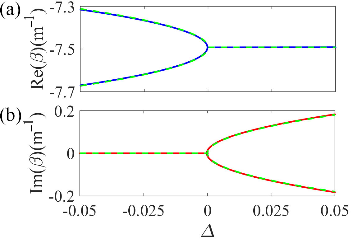
Figure 5: The Puiseux fractional power series expansion in Eq. (12) (green dashed lines) describes the bifurcation of the real and imaginary parts of the two wavenumbers when a system parameter ($\delta_{\mathrm{c}}$ in this case) is perturbed. The Puiseux series result is in excellent agreement with the wavenumbers evaluated using Eq. (10) (blue and red solid lines).

IV Conclusion

A single STM-TL supports EPDs of second order directly induced by spatiotemporal modulation of the distributed (per-unit-length) capacitance. For its occurrence, an EPD does not need the presence of time-invariant gain or loss elements, as in PT symmetry, and it does not need two coupled transmission lines either. Here space and time modulation are not used to generate nonreciprocity or to enhance EPD properties but rather as a direct way to generate EPDs. This is in analogy to what was shown in [4] where time modulation was used to directly induce EPDs in a single resonator, without the need to resorting to two couple resonators with loss and gain as implied by PT-symmetry [7]. We have investigated how to perturb an EPD condition by slightly perturbing system parameters, and how this perturbation modifies the degenerate eigenvalues. We have shown that small changes in a TL constitutive parameters lead to a very strong variation of the TL wavenumber and how this is predicted by the Puiseux fractional expansion series, suggesting a novel approach to design extremely sensitive sensors based on waveguide propagation.

V Acknowledgment

This material is based upon work supported by the National Science Foundation under Grant No. ECCS-1711975.

References

- [1] A. Figotin and I. Vitebskiy, “Oblique frozen modes in periodic layered media,” Physical Review E, vol. 68, no. 3, p. 036609, Sep 2003.
- [2] M. Y. Nada, M. A. K. Othman, and F. Capolino, “Theory of coupled resonator optical waveguides exhibiting high-order exceptional points of degeneracy,” Physical Review B, vol. 96, no. 18, p. 184304, Nov 2017.
- [3] M. A. K. Othman, F. Yazdi, A. Figotin, and F. Capolino, “Giant gain enhancement in photonic crystals with a degenerate band edge,” Physical Review B, vol. 93, no. 2, p. 024301, Jan 2016.
- [4] H. Kazemi, M. Y. Nada, T. Mealy, A. F. Abdelshafy, and F. Capolino, “Exceptional points of degeneracy induced by linear time-periodic variation,” Physical Review Applied, vol. 11, no. 1, p. 014007, Jan 2019.
- [5] C. M. Bender and S. Boettcher, “Real spectra in non-hermitian hamiltonians having PT symmetry,” Physical Review Letters, vol. 80, no. 24, pp. 2455–2464, Jun 1998.
- [6] W. D. Heiss, “Exceptional points of non-hermitian operators,” Journal of Physics A: Mathematical and General, vol. 37, no. 6, pp. 2455–2464, Jan 2004.
- [7] J. Schindler, A. Li, M. C. Zheng, F. M. Ellis, and T. Kottos, “Experimental study of active LRC circuits with PT symmetries,” Physical Review A, vol. 84, no. 4, p. 040101, Oct 2011.
- [8] H. Hodaei, M.-A. Miri, M. Heinrich, D. N. Christodoulides, and M. Khajavikhan, “Parity-time symmetric microring lasers,” Science, vol. 346, no. 6212, pp. 975–978, Nov 2014.
- [9] M. V. Berry, “Physics of nonhermitian degeneracies,” Czechoslovak journal of physics, vol. 54, no. 10, pp. 1039–1047, Oct 2004.
- [10] A. Figotin and I. Vitebskiy, “Gigantic transmission band-edge resonance in periodic stacks of anisotropic layers,” Physical Review E, vol. 72, no. 3, p. 036619, Sep 2005.
- [11] M. A. K. Othman and F. Capolino, “Theory of exceptional points of degeneracy in uniform coupled waveguides and balance of gain and loss,” IEEE Transactions on Antennas and Propagation, vol. 65, no. 10, pp. 5289–5302, Oct 2017.
- [12] A. F. Abdelshafy, M. A. K. Othman, D. Oshmarin, A. T. Almutawa, and F. Capolino, “Exceptional points of degeneracy in periodic coupled waveguides and the interplay of gain and radiation loss: Theoretical and experimental demonstration,” IEEE Transactions on Antennas and Propagation, vol. 67, no. 11, pp. 6909–6923, Nov 2019.
- [13] T. Kato, Perturbation Theory for Linear Operators, 2nd ed. Springer-Verlag, Berlin Heidelberg, 1995, vol. 132.
- [14] M. A. K. Othman, V. A. Tamma, and F. Capolino, “Theory and new amplification regime in periodic multimodal slow wave structures with degeneracy interacting with an electron beam,” IEEE Transactions on Plasma Science, vol. 44, no. 4, pp. 594–611, Apr 2016.
- [15] A. F. Abdelshafy, M. A. K. Othman, F. Yazdi, M. Veysi, A. Figotin, and F. Capolino, “Electron-beam-driven devices with synchronous multiple degenerate eigenmodes,” IEEE Transactions on Plasma Science, vol. 46, no. 8, pp. 3126–3138, Aug 2018.
- [16] M. Veysi, M. A. K. Othman, A. Figotin, and F. Capolino, “Degenerate band edge laser,” Physical Review B, vol. 97, no. 19, p. 195107, May 2018.
- [17] J. Wiersig, “Sensors operating at exceptional points: General theory,” Physical Review A, vol. 93, no. 3, p. 033809, Mar 2016.
- [18] P.-Y. Chen, M. Sakhdari, M. Hajizadegan, Q. Cui, M. M.-C. Cheng, R. El-Ganainy, and A. Alu, “Generalized parity-time symmetry condition for enhanced sensor telemetry,” Nature Electronics, vol. 1, no. 5, pp. 297–304, May 2018.
- [19] H. Kazemi, M. Y. Nada, F. Maddaleno, and F. Capolino, “Experimental demonstration of exceptional points of degeneracy in linear time periodic systems and exceptional sensitivity,” arXiv preprint arXiv:1908.08516, 2019.
- [20] H. Kazemi, A. Hajiaghajani, M. Y. Nada, M. Dautta, M. Alshetaiwi, P. Tseng, and F. Capolino, “Ultra-sensitive radio frequency biosensor at an exceptional point of degeneracy induced by time modulation,” arXiv preprint arXiv:1909.03344, 2019.
- [21] E. S. Cassedy and A. A. Oliner, “Dispersion relations in time-space periodic media: Part I–stable interactions,” Proceedings of the IEEE, vol. 51, no. 10, pp. 1342–1359, Oct 1963.
- [22] E. S. Cassedy, “Dispersion relations in time-space periodic media Part II–unstable interactions,” Proceedings of the IEEE, vol. 55, no. 7, pp. 1154–1168, Jul 1967.
- [23] C. Elachi, “Electromagnetic wave propagation and wave-vector diagram in space-time periodic media,” IEEE Transactions on Antennas and Propagation, vol. 20, no. 4, pp. 534–536, Jul 1972.
- [24] J. R. Zurita-Sanchez, P. Halevi, and J. C. Cervantes-Gonzalez, “Reflection and transmission of a wave incident on a slab with a time-periodic dielectric function (t),” Physical Review A, vol. 79, no. 5, p. 053821, May 2009.
- [25] J. S. Martínez-Romero, O. M. Becerra-Fuentes, and P. Halevi, “Temporal photonic crystals with modulations of both permittivity and permeability,” Physical Review A, vol. 93, no. 6, p. 063813, Jun 2016.
- [26] N. A. Estep, D. L. Sounas, and A. Alu, “Magnetless microwave circulators based on spatiotemporally modulated rings of coupled resonators,” IEEE Transactions on Microwave Theory and Techniques, vol. 64, no. 2, pp. 502–518, Feb 2016.
- [27] S. Taravati and C. Caloz, “Mixer-duplexer-antenna leaky-wave system based on periodic space-time modulation,” IEEE Transactions on Antennas and Propagation, vol. 65, no. 2, pp. 442–452, Feb 2017.
- [28] H. Rajabalipanah, A. Abdolali, and K. Rouhi, “Reprogrammable spatiotemporally modulated graphene-based functional metasurfaces,” IEEE Journal on Emerging and Selected Topics in Circuits and Systems, vol. 10, no. 1, pp. 75–87, Mar 2020.
- [29] S. Qin, Q. Xu, and Y. E. Wang, “Nonreciprocal components with distributedly modulated capacitors,” IEEE Transactions on Microwave Theory and Techniques, vol. 62, no. 10, pp. 2260–2272, Oct 2014.
- [30] K. A. Lurie and V. V. Yakovlev, “Energy accumulation in waves propagating in space- and time-varying transmission lines,” IEEE Antennas and Wireless Propagation Letters, vol. 15, pp. 1681–1684, Jan 2016.
- [31] N. Reiskarimian, M. B. Dastjerdi, J. Zhou, and H. Krishnaswamy, “Analysis and design of commutation-based circulator-receivers for integrated full-duplex wireless,” IEEE Journal of Solid-State Circuits, vol. 53, no. 8, pp. 2190–2201, Aug 2018.
- [32] F. Wu, Y. Zheng, F. Yuan, and Y. Fu, “Magnetic-free isolators based on time-varying transmission lines,” Electronics, vol. 8, no. 6, p. 684, Jun 2019.
- [33] X. Wu, X. Liu, M. D. Hickle, D. Peroulis, J. S. Gomez-Diaz, and A. A. Melcon, “Isolating bandpass filters using time-modulated resonators,” IEEE Transactions on Microwave Theory and Techniques, vol. 67, no. 6, pp. 2331–2345, Jun 2019.
- [34] M. A. K. Othman, M. Veysi, A. Figotin, and F. Capolino, “Low starting electron beam current in degenerate band edge oscillators,” IEEE Transactions on Plasma Science, vol. 44, no. 6, pp. 918–929, Jun 2016.
- [35] Z. Yu and S. Fan, “Complete optical isolation created by indirect interband photonic transitions,” Nature Photonics, vol. 3, no. 2, pp. 91–94, Feb 2009.
- [36] A. Figotin and I. Vitebskiy, “Slow-wave resonance in periodic stacks of anisotropic layers,” Physical Review A, vol. 76, no. 5, p. 053839, Nov 2007.
- [37] J. Moro, J. V. Burke, and M. L. Overton, “On the Lidskii–Vishik–Lyusternik perturbation theory for eigenvalues of matrices with arbitrary Jordan structure,” SIAM Journal on Matrix Analysis and Applications, vol. 18, no. 4, pp. 793–817, Oct 1997.
- [38] A. Welters, “On explicit recursive formulas in the spectral perturbation analysis of a Jordan Block,” SIAM Journal on Matrix Analysis and Applications, vol. 32, no. 1, pp. 1–22, Jan 2011.
- [39] G. W. Hanson, A. B. Yakovlev, M. A. Othman, and F. Capolino, “Exceptional points of degeneracy and branch points for coupled transmission lines—linear-algebra and bifurcation theory perspectives,” IEEE Transactions on Antennas and Propagation, vol. 67, no. 2, pp. 1025–1034, Feb 2019.
- [40] W. Chen, S. Kaya Ozdemir, G. Zhao, J. Wiersig, and L. Yang, “Exceptional points enhance sensing in an optical microcavity,” Nature, vol. 548, no. 7666, pp. 192–196, Aug 2017.
- [41] H. Hodaei, A. U. Hassan, S. Wittek, H. Garcia-Gracia, R. El-Ganainy, D. N. Christodoulides, and M. Khajavikhan, “Enhanced sensitivity at higher-order exceptional points,” Nature, vol. 548, no. 7666, pp. 187–191, Aug 2017.
- [42] F. Ellinger, H. Jackel, and W. Bachtold, “Varactor-loaded transmission-line phase shifter at c-band using lumped elements,” IEEE Transactions on Microwave Theory and Techniques, vol. 51, no. 4, pp. 1135–1140, Apr 2003.
- [43] K. Rouhi, H. Rajabalipanah, and A. Abdolali, “Multi-bit graphene-based bias-encoded metasurfaces for real-time terahertz wavefront shaping: From controllable orbital angular momentum generation toward arbitrary beam tailoring,” Carbon, vol. 149, pp. 125–138, Aug 2019.
- [44] A. Komar, R. Paniagua-Domínguez, A. Miroshnichenko, Y. F. Yu, Y. S. Kivshar, A. I. Kuznetsov, and D. Neshev, “Dynamic beam switching by liquid crystal tunable dielectric metasurfaces,” ACS Photonics, vol. 5, no. 5, pp. 1742–1748, Feb 2018.